

Abstract
Conventional x-ray computed tomography (CT) scanners are limited in their scanning speed by the mechanical constraints of their rotating gantries and as such do not provide the necessary temporal resolution for imaging of fast-moving dynamic processes, such as moving fluid flows. The Real Time Tomography (RTT) system is a family of fast cone beam CT scanners which instead use multiple fixed discrete sources and complete rings of detectors in an offset geometry. We demonstrate the potential of this system for use in the imaging of such high speed dynamic processes and give results using simulated and real experimental data. The unusual scanning geometry results in some challenges in image reconstruction, which are overcome using algebraic iterative reconstruction techniques and explicit regularisation. Through the use of a simple temporal regularisation term and by optimising the source firing pattern, we show that temporal resolution of the system may be increased at the expense of spatial resolution, which may be advantageous in some situations. Results are given showing temporal resolution of approximately 500 µs with simulated data and 3 ms with real experimental data.
Export citation and abstract BibTeX RIS

Content from this work may be used under the terms of the Creative Commons Attribution 3.0 licence. Any further distribution of this work must maintain attribution to the author(s) and the title of the work, journal citation and DOI.
1. Introduction
Conventionally, medical x-ray tomographic imaging systems have used a single x-ray source and an array of detectors which together rotate around the object of interest to form a set of x-ray projections through the object. These projections can be reconstructed to form an image of the object in either two or three dimensions, depending on whether the detector configuration is single row fan beam or multi-row cone beam. Equivalently, laboratory based x-ray micro CT scanners also use a single source, but in this case, the object is rotated while the source and detector are kept stationary.
The main factor limiting the speed of these conventional single-source systems is the physical rotation of the source or object. Due to the mass of the gantry, typical modern medical CT scanners can experience centripetal acceleration of up to 30g [1], which restricts scan rates to only a few source revolutions per second. The latest dual source medical CT scanners are able to perform just over 3 s−1 [2], giving a reconstructed image frame rate of less than 10 s−1. In some applications, such frame rates are too slow to provide the required temporal resolution; for example in the visualisation of the flow of liquids or granular materials.
To address this problem, it is necessary to eliminate the mechanical scanning motion, replacing this with an electronic equivalent comprising a circular array of x-ray sources which can be fired individually under computer control. By switching the sources in sequence, the equivalent of movement can be generated without physical motion of any component of the system.
A Real Time Tomography (RTT) system has been developed to solve this technological problem [3, 4], in which an approximately circular array of x-ray sources over an angular distribution of 180° plus fan angle is matched with a corresponding array of x-ray detectors to provide an x-ray tomographic scanning system with no moving parts. The plane containing the x-ray sources is offset from the plane containing the x-ray detectors to avoid the beam having to pass through detectors before it is transmitted through the object under inspection.
The x-ray sources comprise an array of electron guns, each of which is controlled by an independent electronic switching circuit. These switching circuits can be pulsed in microsecond timescales. The electron beam from a given source is accelerated through a high potential difference to a tungsten coated anode to produce x-rays. A single distributed anode is arranged in a circular configuration such that each electron gun irradiates a different region of the anode around the circle or polygon, resulting in an effective x-ray focus when viewed from the detectors of typically 1 mm2. The electron gun control electronics can be programmed to irradiate the electron guns in any given sequence. Therefore, this is a flexible data acquisition platform and is capable of generating tomographic scan data at theoretical source rotation rates of up to 480 frames per second.
So far, RTT systems have been produced in three sizes; a prototype system with 20 cm tunnel and a single ring of detectors and production models with 80 cm and 110 cm tunnel diameters, using multiple detector rings. The larger production systems were designed for application in airport security, in order to provide fast three-dimensional imaging of baggage as it passes through on a conveyor belt at up to 0.5 m s−1. In this application, the third dimension is used to provide z information rather than time; the resulting reconstruction process is a different problem than that discussed in detail in this work, but owing to the offset geometry, this has necessitated development of new algorithms. A fast Feldkamp based approximate 3D back projection algorithm has been developed for real-time reconstruction [5] and the use of algebraic iterative methods has been investigated as part of a scheme for artefact reduction [6]. An efficient algorithm based on rebinning to multi-sheet surfaces has also been proposed [7, 8]; this has recently been implemented for real-time reconstruction and has been shown to work well, requiring less computational resources than the fully 3D approaches. The 3D reconstruction problem will not be discussed further in this work.
2. The RTT20 system
RTT20 is a small-scale prototype RTT system which has been acquired by the University of Manchester for the Manchester X-ray Imaging Facility. Intended applications at the University include the study of moving multi-phase fluid flows and granular flows, with the aim of experimentally validating theoretical models. The machine consists of a tunnel of diameter 20 cm (hence RTT20), with an internal conveyor belt for positioning the sample in the plane of the x-ray beams (see figure 1); the multiple source x-ray tube and detector rings are positioned around the tunnel.
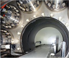
Figure 1. View of the RTT20 tunnel and conveyor belt, showing the vacuum tube and electron gun assembly.
Download figure:
Standard image High-resolution imageFigure 2 shows the RTT20 source and detector geometry in first angle orthographic projection; a standard right-handed cartesian coordinate system is defined, with the origin at the isocentre of the system. Sources are located in the plane z = 0, with the detector offset in the direction of the positive z-axis; note that the z scale in the figure is highly exaggerated in order to show the offset source-detector geometry. The sources are arranged in 8 blocks of 32, with two 'missing' blocks of sources at the bottom; this incomplete ring geometry is part of the original prototype design to enable a small scanner to be easily fixed onto pipes for imaging flowing fluids. The two blocks adjacent to the gap do not use their outermost 4 sources, giving a total of 248 sources. There is one full ring of detectors arranged in 21 blocks of 16, giving 336 detectors in total; this is offset from the source plane by 5.48 mm in the z direction.
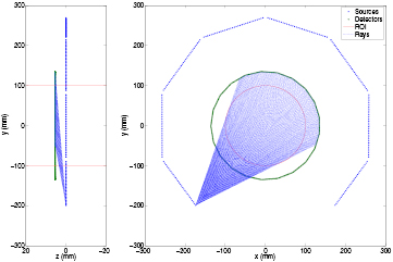
Figure 2. The RTT20 geometry, showing locations of the sources, detectors and scanned region (left: y–z cross-section with exaggerated z scale to show offset between source and detector planes; right: x–y cross-section).
Download figure:
Standard image High-resolution imageThe machine is capable of acquiring a complete set of projections from all 248 sources 60 times per second; a complete set of projections is referred to as a revolution. Sources may be fired in almost any order we desire; the only constraints are imposed due to thermal limitations of the individual sources. For a general RTT system with N sources, this is defined by some function, or sequence of functions

known as a firing order. In order to use all sources and therefore fully sample the available projection angles within each revolution, the function used is generally bijective. The firing order originally used for the prototype RTT20 system is defined for 256 sources by the function
The first and last four sources in the sequence are simply removed to reduce this to firing only the 248 sources which are actually used.
3. Reconstruction
3.1. Reconstruction of dynamic RTT data sets
When scanning an object or dynamic process, the RTT20 system operates continuously; therefore an RTT20 dynamic data set consists of a number of full sets of 248 projections, each recorded sequentially with no gaps in between. The reconstruction of an RTT20 dynamic data set forms a sequence of images, each of which is referred to as a frame.
The simplest method of reconstruction is to regard each complete set of 248 projections as representing a frame and reconstruct each one of these independently. For applications where the motion of the object is slow compared to the data collection rate this may be adequate. However, if the firing order is chosen appropriately, so that the distribution of projection angles is even for smaller subsets of projections, then we may divide each full set of projections to represent multiple frames. This effectively trades contrast and spatial resolution for temporal resolution. The firing order described by equation (2), whilst not optimal in the sense discussed in section 3.6, satisfies this condition to some extent. Note that reconstructing frames independently takes no account of possible correlations in the motion between consecutive frames.
The process of independently reconstructing each two-dimensional frame is simple and well-understood; however, the construction of RTT20 presents some problems. Firstly, the polygonal nature of the source and detector rings means that the distribution of projection angles and the angles of rays within each projection, are somewhat uneven. This, combined with the incomplete source ring, causes an uneven sampling of the two-dimensional Radon transform; this is shown in figure 3.
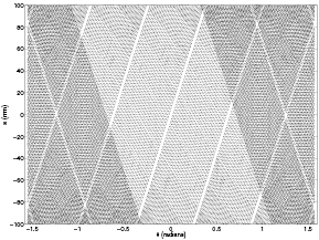
Figure 3. Distribution of sampling points in the 2D Radon transform space.
Download figure:
Standard image High-resolution imageSecondly, the offset detector means that we do not really measure rays in a plane through the object. However, compared to the x–y resolution of the system, the effect of the offset is considered small enough to ignore within the reconstruction region of interest. To illustrate this, figure 4 shows the range of z values covered by the rays intersecting each voxel within the reconstruction region, giving a measure of expected z-axis resolution. Clearly the planar approximation works well in the centre of the region of interest, but weakens towards the edges.
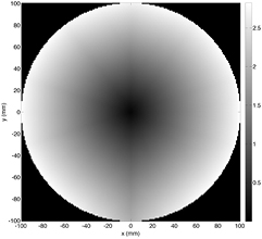
Figure 4. Range of z-axis deviation per voxel within the ROI, showing the accuracy of the planar approximation. Values represent the maximum absolute difference in z for all rays intersecting each x–y voxel (units in mm).
Download figure:
Standard image High-resolution image3.2. Analytical algorithms
Analytical reconstruction algorithms based on filtered back projection (FBP) for the 2D fan beam geometry are well-known [9]. However, these assume an equal spacing of the projection angles and either an equiangular or equally spaced linear sampling scheme for the rays within each projection. Therefore, due to the construction of RTT20, with its polygonal source and detector rings, an interpolation to the parallel beam geometry can be used.
For applications where fast reconstruction is important, such as real time observation of flow through an oil pipe, or monitoring of an experiment in progress, taking all 248 projections per frame and using filtered back projection gives adequate results. However, the performance of filtered back projection degrades significantly if the number of projections per frame is reduced; therefore, for fast moving objects, motion artefacts will be observed.
3.3. Algebraic iterative reconstruction
Algebraic iterative reconstruction methods are based on forming a discrete representation of the projection process and then solving the resulting system of linear equations iteratively. Well-known algorithms from numerical linear algebra, such as Kaczmarz' method [10] and Cimmino's [11] or Landweber's method [12], are known widely for their application to CT reconstruction as ART [13] and SIRT [14]. Many other variants and refinements of these basic algorithms have been developed specifically for CT problems. We may also use more advanced numerical algorithms, with theoretically faster convergence rates, such as conjugate gradient least squares (CGLS) [15],
These methods offer some advantages over filtered back projection; firstly, no assumptions are made about the scanning geometry and secondly, performance of such algorithms tends to be better than filtered back projection when the data set consists of fewer projections. However, the computational demands of algebraic iterative reconstruction techniques are much higher, resulting in slower reconstruction times. This effectively prevents their use for applications requiring real time reconstruction, at least on currently available hardware, but for applications where the data acquisition and image analysis processes are separate, such as detailed analysis of experimental data, this is not a significant problem.
We let the matrix A represent the projection process for each complete set of 248 projections; this may represent more than one frame and is simply re-used for each projection set. A simple length of intersection model is used for the projection process, with the elements of A being calculated using the ray tracing algorithm of Jacobs et al [16], which is itself a development of Siddon's algorithm [17]. In order to take the offset geometry into account, ray tracing is performed in 3D; to ensure only a single slice is considered, the voxels are simply defined to be long in the z direction. This has been implemented in MATLAB as a C .mex routine, with output in the MATLAB double precision sparse matrix format. Using 1 mm × 1 mm × 10 mm voxels covering the entire circular ROI, storage requirements for A are approximately 100 MB.
For each complete set of projections, the system of equations Ax = b is solved using CGLS. We use the MATLAB implementation of CGLS provided in Hansen's Regularization Tools package [18].
3.4. Regularisation
Although regularisation can be added to the filtered back projection algorithm by changing the frequency response of the filter, algebraic reconstruction methods allow regularisation to be built in with far greater flexibility. Indeed, for CGLS or any of the other commonly used iterative methods such as Kaczmarz or Landweber, the number of iterations plays the role of a regularisation parameter when applied to the system of equations without adding explicit regularisation.
However, such regularisation is not systematic, so the exact effect is unclear. It is also often unclear how many iterations should be performed in order to provide the correct degree of regularisation. We may therefore apply systematic regularisation by solving the augmented system of equations
in the least squares sense and iterating to convergence, where α is a regularisation parameter, L is some finite difference approximation to a differential operator and 0 is the zero vector of length equal to the total number of image voxels. This gives the least squares solution
The matrix L defines a penalty term on the solution and may be chosen to penalise solutions with certain properties. For example, if L is chosen as an operator which increases the high spatial frequency content, for example the Laplacian, then a smooth solution will be enforced. The degree of smoothing is controlled with the regularisation parameter α. This can also be interpreted in the Bayesian sense, where the solution x is the MAP estimate with Gaussian prior and α2 LT L is the inverse covariance matrix.
For objects of a piecewise constant structure, with a sparse representation in the gradient domain, regularisation based on the L1-norm has been demonstrated to give improved results when the angular sampling rate is low [19, 20]. This type of regularisation tends to smooth out noise in the reconstructed images while preserving sharp edges and is anticipated to be an important direction for future research.
3.5. Temporal regularisation
By considering the data set as a whole, rather than representing a set of discrete independent frames, regularisation can also be added in the temporal dimension, allowing correlation between consecutive frames to be taken into account. The matrix Atotal, representing the whole system, is formed from A by a Kronecker product with the identity matrix of size equal to the number of complete projection sets. We can then solve an augmented system of equations as in (3). This is a simple process and can be implemented efficiently.
Regularisation has been performed by taking L to be the three-dimensional discrete Laplacian. By incorporating the regularisation parameter into the matrix L, it is possible to choose differing amounts of regularisation in the spatial and temporal dimensions. Letting m and n be the number of image pixels in the x and y directions respectively and letting p be the number of frames, L has the following Kronecker product decomposition:

where Im is the m × m identity matrix, Dm is the one-dimensional discrete Laplacian on m points and αs and αt are respectively the spatial and temporal regularisation parameters.
3.6. Optimising the firing order
We wish to choose the firing order so as to optimise the spread of projection angles representing each frame. In the case of neutron tomography of dynamic processes where the choice of projection angle is effectively continuous, it has been shown in [21], based on results from [22], that by choosing successive projections based on the golden ratio  , any subset of the full set of projection angles gives an even coverage of angles in [0, π]. In this scheme, projection angles θi are chosen according to

In the case of an RTT system, with discrete sources, the set of projection angles is finite. However, we may approximate this scheme by using a firing order of the form

where N is the total number of sources in the system and k is some integer coprime to N, chosen so as to approximate N/φ, where φ is the golden ratio. For RTT20, with N = 248, we use k = 153.
Note that if the firing order is chosen in this way, the choice of how many projections to use for each frame and therefore the tradeoff between spatial and temporal resolution, in the final reconstruction may be taken after the data have been collected, since the spread of projection angles for larger subsets of projections is still even.
4. Results
4.1. Simulated data
Simulated data were generated for a ball of radius 10 mm, with unit CT attenuation coefficient, moving horizontally along a line through the centre of the scanner in a sinusoidal motion of frequency 2Hz and amplitude 80 mm against a zero background. Ray integrals were calculated analytically assuming a mono-energetic spectrum, with the object position being re-calculated for each projection. Simulations were performed at the scanner's standard speed of 60 full sets of 248 projections per second, using the firing order described by equation (2) and also the firing order of equation (7), using k = 153. The two firing orders are referred to as respectively original and optimal and are defined explicitly by the functions

Data were corrupted with Poisson noise, assuming a photon count of 104 after conversion to transmission data.
Figure 5 compares a frame from reconstructions of the simulated data calculated with both of the firing orders represented by equations (8) and (9). Varying reconstruction parameters are used, with 248, 31 and 8 projections per frame (respectively 1, 8 and 31 frames per full projection set). The selected frame was chosen so as to lie as close as possible to the centre of the motion, where the motion is at its fastest. Figures 6 and 7 show respectively the 2-norms of the residual (data error) and difference from the reference ground truth image (image error) at each iteration, for the first 50 iterations. Additionally, tables 1 and 2 give the minimum image error values in each case and their corresponding iteration numbers.
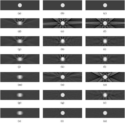
Figure 5. Reconstructed images of a single frame from the simulated data (left column: 248 projections per frame; centre column: 31 projections per frame; right column: 8 projections per frame; (d)–(l): original firing order; (m)–(u): optimal firing order). (a) Ground truth. (b) Ground truth. (c) Ground truth. (d) FBP. (e) FBP. (f) FBP. (g) CGLS, αt = 0, nit = 5. (h) CGLS, αt = 0, nit = 66. (i) CGLS, αt = 0, nit = 100. (j) CGLS, αt = 1.3, nit = 5. (k) CGLS, αt = 1.0, nit = 78. (l) CGLS, αt = 5.9, nit = 100. (m) FBP. (n) FBP. (o) FBP. (p) CGLS, αt = 0, nit = 6. (q) CGLS, αt = 0, nit = 100. (r) CGLS, αt = 0, nit = 100. (s) CGLS, αt = 1.3, nit = 7. (t) CGLS, αt = 1.0, nit = 37. (u) CGLS, αt = 5.9, nit = 100.
Download figure:
Standard image High-resolution image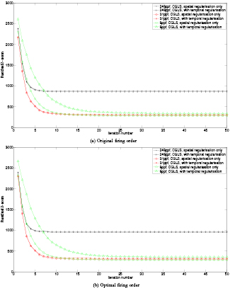
Figure 6. Data error 2-norms for the simulated data reconstructions. (a) Original firing order. (b) Optimal firing order.
Download figure:
Standard image High-resolution image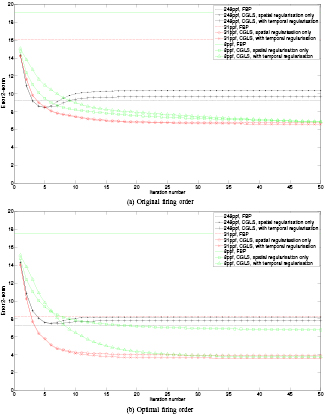
Figure 7. Image error 2-norms for the simulated data reconstructions. (a) Original firing order. (b) Optimal firing order.
Download figure:
Standard image High-resolution imageTable 1. Minimum error values and corresponding iteration numbers for the original firing order.
| Minimum error value | At iteration number | |
|---|---|---|
| 248ppf, FBP | 9.27 | N/A |
| 248ppf, CGLS, spatial reg. only | 8.48 | 5 |
| 248ppf, CGLS, temporal reg. | 8.45 | 5 |
| 31ppf, FBP | 16.11 | N/A |
| 31ppf, CGLS, spatial reg. only | 6.70 | 66 |
| 31ppf, CGLS, temporal reg. | 6.54 | 78 |
| 8ppf, FBP | 19.10 | N/A |
| 8ppf, CGLS, spatial reg. only | 6.29 | 100 |
| 8ppf, CGLS, temporal reg. | 5.99 | 100 |
Table 2. Minimum error values and corresponding iteration numbers for the optimal firing order.
| Minimum error value | At iteration number | |
|---|---|---|
| 248ppf, FBP | 7.29 | N/A |
| 248ppf, CGLS, spatial reg. only | 7.52 | 6 |
| 248ppf, CGLS, temporal reg. | 7.48 | 6 |
| 31ppf, FBP | 8.26 | N/A |
| 31ppf, CGLS, spatial reg. only | 3.91 | 100 |
| 31ppf, CGLS, temporal reg. | 3.64 | 37 |
| 8ppf, FBP | 17.51 | N/A |
| 8ppf, CGLS, spatial reg. only | 6.63 | 100 |
| 8ppf, CGLS, temporal reg. | 3.75 | 100 |
In each case, comparisons were performed between the ground truth image, filtered back projection reconstruction and CGLS reconstructions both with and without temporal regularisation. Filtered back projection reconstructions used the equiangular fan beam algorithm, with Parker weighting for data redundancy [23]. In all CGLS cases, the spatial regularisation parameter was chosen as αs = 3.75, this value being determined by minimising the 2-norm of the difference between 248 projection reconstructions of a static ball centred at the origin and its ground truth image.
In the cases where temporal regularisation was used, the value of the temporal regularisation parameter αt was again chosen by minimising the 2-norm of the difference between the reconstruction and ground truth image. A similar procedure was also used to determine the optimal number of iterations. Obviously, this method of parameter selection is only applicable with synthetic data; for practical use cases with experimental data, current methods are purely empirical. This is an important area for future research; it is possible that a method such as L-curve [24] could be used.
We see that for this data set, using all 248 projections per frame results in strong motion artefacts. By reducing the number of projections per frame, motion artefacts are eliminated, but with no temporal regularisation, streak artefacts are observed. As expected, filtered back projection performs poorly; even with no temporal regularisation, the artefacts observed in CGLS reconstructions are much weaker.
By introducing temporal regularisation, streak artefacts are much reduced and acceptable reconstructions can be obtained with as few as 8 projections per frame, with a corresponding 31 × increase in temporal resolution, where temporal resolution is simply defined as the length of time taken to collect the projection data for a single frame. By reducing the number of projections per frame in this way, the motion between subsequent frames is reduced so that it makes sense to smooth in the temporal dimension. Additionally, using the optimised firing order provides a more even distribution of the projection angles and reduces the artefacts further. Figure 8 shows time domain visualisations of the temporally regularised reconstructions in the cases of 248, 31 and 8 projections per frame, demonstrating the increased temporal resolution that can be achieved.
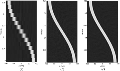
Figure 8. Visualisations of the simulated data CGLS reconstructions in the time domain, in the case of the optimal firing order including temporal regularisation. The images show time on the vertical axis against the spatial x dimension, at a constant spatial y value of −0.5 mm. (a) 248 projections per frame. (b) 31 projections per frame. (c) 8 projections per frame.
Download figure:
Standard image High-resolution image4.2. Real data
Real experimental data were available for a scan of a mixture of oil, water and air moving in a bottle. The data set consists of 61 full projection sets representing 1 s of the motion and was collected during the machine's initial testing process. The scanner settings used were a voltage of 120 keV and current of 10 mA. Three of the sources in the prototype scanner were defective, resulting in a total of 245 working sources. All collected data used the original firing order of equation (2), with the defective sources removed from the sequence.
Figure 9 compares a frame from reconstructions of the data made with filtered back projection and CGLS with and without temporal regularisation. Comparisons are shown for a full set of 245 projections per frame and 49 projections per frame (5 frames per full projection set). In all CGLS cases, 100 iterations were performed and the spatial regularisation parameter was again chosen as αs = 3.75. Temporal regularisation parameters were chosen empirically, by performing test reconstructions of a small number of frames at a range of parameter values and selecting the minimum value that effectively reduced artefacts in each case, in order to avoid over-smoothing. The values chosen for the two data sets were respectively αt = 10 and αt = 50. We would expect the optimal parameter value to vary depending on the number of projections used per frame, the firing order and the amount and speed of motion in the sample. In this case, we are able to choose a relatively high value of αt due to the slow rate of the motion compared to the data acquisition rate.
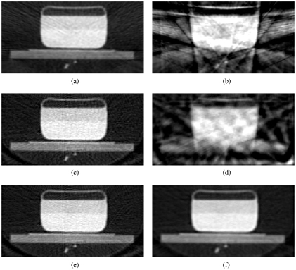
Figure 9. Reconstructed images of a single frame from the oil and water data (left, 245 projections; right, 49 projections). (a) FBP. (b) FBP. (c) CGLS, αt = 0. (d) CGLS, αt = 0. (e) CGLS, αt = 10. (f) CGLS, αt = 50.
Download figure:
Standard image High-resolution imageAs before, filtered back projection reconstructions use the equiangular fan beam algorithm with Parker weighting. The prototype machine used also had three defective detectors. For the CGLS reconstructions, the corresponding entries in the projection matrix were simply set to zero, whereas for the filtered back projection reconstructions, the values corresponding to these detectors were filled in by linear interpolation between the two neighbouring detectors.
The motion in this case is not as fast as the simulated data and reasonable results are obtained by simply using all 245 projections per frame. However, by using only 49 projections per frame and applying temporal regularisation, temporal resolution has increased by a factor of 5; this improvement is more noticeable when viewing the full dynamic reconstruction as a video. Although the 49 projection temporally regularised images are noticeably softer than those using the full set of projections per frame, they compare well and in certain applications the gain in temporal resolution may be more important.
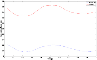
As an example of how reconstructions of dynamic RTT data may be used in practice, figure 10 shows plots of the mean height of the water-oil and oil-air interfaces, measured across the width of the container. These were extracted from the 49 projections per frame temporally regularised CGLS reconstruction using a simple thresholding segmentation algorithm. The process of extracting moving features such as these from dynamic reconstructions is a research topic in itself and will not be discussed further here.
Figure 10. Mean surface heights extracted from reconstruction of the oil and water data.
Download figure:
Standard image High-resolution image
5. Conclusions
We have introduced the concept of the RTT system, as applied to the problem of imaging fast-moving dynamic processes, such as fluid and granular flows. Problems caused by the highly uneven sampling generated by the system's geometry have been solved by using algebraic iterative reconstruction and explicit regularisation, rather than the more widely used filtered back projection based algorithms.
By implementing a simple temporal regularisation process based on the three-dimensional discrete Laplacian and by optimising the system's source firing pattern, we have demonstrated the potential to reconstruct dynamic data sets with as few as eight projections per frame, giving a temporal resolution of approximately 500 µs. Although temporal resolution this high has so far only been demonstrated with simulated data, our results with real data have shown that temporal resolution can be increased in real world applications by at least a factor of 5.
Through our results with the oil and water data, we were able to track the surface heights of the interfaces between the fluids at a temporal resolution of approximately 3 ms. This clearly demonstrates the potential of the RTT system to provide novel images of moving fluid flows and other fast-moving dynamic processes. Plans for future work are to collaborate with fluid and granular flow theorists in order to design experiments to be performed in an RTT110 system and to apply our reconstruction techniques to these. We also intend to apply L1-norm based regularisation techniques to the reconstruction process.
Acknowledgments
We would like to thank Rapiscan Systems Ltd. and EPSRC (grant EP/E010997/1) for supporting this work. In particular, we would like to thank the RTT development team for providing us with access to technical details of the system and experimental data.