
Abstract
All imaging modalities such as computed tomography, emission tomography and magnetic resonance imaging require a reconstruction approach to produce an image. A common image processing task for applications that utilise those modalities is image segmentation, typically performed posterior to the reconstruction. Recently, the idea of tackling both problems jointly has been proposed. We explore a new approach that combines reconstruction and segmentation in a unified framework. We derive a variational model that consists of a total variation regularised reconstruction from undersampled measurements and a Chan–Vese-based segmentation. We extend the variational regularisation scheme to a Bregman iteration framework to improve the reconstruction and therefore the segmentation. We develop a novel alternating minimisation scheme that solves the non-convex optimisation problem with provable convergence guarantees. Our results for synthetic and real data show that both reconstruction and segmentation are improved compared to the classical sequential approach.
Export citation and abstract BibTeX RIS

Original content from this work may be used under the terms of the Creative Commons Attribution 3.0 licence. Any further distribution of this work must maintain attribution to the author(s) and the title of the work, journal citation and DOI.
1. Introduction
Image reconstruction plays a central role in many imaging modalities for medical and non-medical applications. The majority of imaging techniques deal with incomplete data and noise, making the inverse problem of reconstruction severely ill-posed. Based on compressed sensing (CS) it is possible to tackle this problem by exploiting prior knowledge of the signal [1–3]. Nevertheless, reconstructions from very noisy and undersampled data will present some errors that will be propagated into further analysis, e.g. image segmentation. Segmentation is an image processing task used to partition the image into meaningful regions. Its goal is to identify objects of interest, based on contours or similarities in the interior. Typically segmentation is performed after reconstruction, hence its result strongly depends on the quality of the reconstruction. Recently the idea of combining reconstruction and segmentation has become more popular. The main motivation is to avoid error propagations that occur in the sequential approach by estimating edges simultaneously from the data, ultimately improving the reconstruction. In this paper, we propose a new model for joint reconstruction and segmentation from undersampled magnetic resonance imaging (MRI) data. The underlying idea is to incorporate prior knowledge about the objects that we want to segment in the reconstruction step, thus introducing additional regularity in our solution. In this unified framework, we expect that the segmentation will also benefit from sharper reconstructions. We demonstrate that our joint approach improves the reconstruction quality and yields better segmentations compared to sequential approaches. In figure 1, we consider a brain phantom from which we simulated the undersampled k-space data and added Gaussian noise. Figures 1(b) and (e) present reconstructions and segmentations obtained with the sequential approaches, while figures 1(c) and (f) show the results for our joint approach. The reconstruction using our method shows clearly more details and it is able to detect finer structures that are not recovered with the classical separate approach. As a consequence, the joint segmentation is also improved. In the following section we present the mathematical models that we used in our comparison. We investigated the performance of our model for two different applications: bubbly flow and cancer imaging. We show that both reconstruction and segmentation benefit from this method, compared to the traditional sequential approaches, suggesting that error propagation is reduced.

Figure 1. Sequential approach (left) versus unified approach (right). Combining reconstruction and segmentation in a single unified approach improves both the reconstructed image and its segmentation. See figure 2 for more details. (a) Groundtruth. (b) Sequential reconstruction. (c) Joint reconstruction. (d) Sampling matrix. (e) Sequential segmentation. (f) Joint segmentation.
Download figure:
Standard image High-resolution imageOur contribution. In our proposed joint method, we obtain an image reconstruction that preserves its intrinsic structures and edges, possibly enhancing them, thanks to the joint segmentation, and simultaneously we achieve an accurate segmentation. We consider the edge-preserving total variation regularisation for both the reconstruction and segmentation term using Bregman distances. In this unified Bregman iteration framework, we have the advantage of improving the reconstruction by reducing the contrast bias in the TV formulation, which leads to more accurate segmentation. In addition, the segmentation constitutes another prior for the reconstruction by enhancing edges of the regions of interest. Furthermore, we propose a non-convex alternating direction algorithm in a Bregman iteration scheme for which we prove global convergence.
The paper is organised as follows. In section 2 we describe the problems of MRI reconstruction and region-based segmentation. We then introduce our joint reconstruction and segmentation approach in a Bregman iteration framework. This section also contains a detailed comparison of other joint models in the literature. In section 3 we study the non-convex optimisation problem and present the convergence analysis for this class of problems. Finally in section 4 we present numerical results for MRI data for different applications. Here we investigate the robustness of our model by testing the undersampling rate up to its limit and by considering different noise levels.
2. MRI reconstruction and segmentation
In the following section we introduce the mathematical tools to perform image reconstruction and image segmentation. In this work, we focus on the specific MRI application; however, our proposed joint method can be applied to other imaging problems in which the measured data is connected to the image via a linear and bounded forward operator, see section 2.1. Finally we present our model that combines the two tasks of reconstruction and segmentation in a unified framework.
2.1. Reconstruction
In image reconstruction problems, we have the general setting

where  is a bounded and linear operator mapping between two vector-spaces. The measured data
  is usually corrupted by some noise
  and often only observed partially. In this formulation we are interested in recovering the image u given the data f .
In this work, we focus on the application of MRI and we refer to the measurements f as the k-space data. In standard MRI acquisitions, the Fourier coefficients are collected in the k-space by radio-frequency (RF) coils. Because the k-space data is acquired sequentially, the scanning time is constrained by physical limitations of the imaging system. One of the most common ways to perform fast imaging consists of undersampling the k-space; this, however, only yields satisfactory results if the dimension of the parameter space can implicitly be reduced, for example by exploiting sparsity in certain domains. In the reconstruction, this assumption is incorporated in the regularisation term. Let  with
with  be a discrete image domain. Let
  with
with  be our given undersampled k-space data, where
  are the measured Fourier coefficients that fulfil the relationship (1) with A = SF. The operator A is now composed by
  , which is a sampling operator that selects m measurements from the Fu data according to the locations provided by a binary sampling matrix (see e.g. figure 1(d)), where F is the discrete Fourier transform. In MRI, the noise
  is drawn from a complex-valued Gaussian distribution with zero mean and standard deviation
  [4].
[4].
In problem (1) for MRI, the aim is to recover the image  from the data. However, in this work we follow the standard assumption that in many applications we have negligible phase, i.e. we are working with real valued, non-negative images. Therefore, we are only interested in
  ; hence we consider the MRI forward operator as
  and its adjoint
  as modelled in [5]. Problem (1) is ill-posed due to noise and incomplete measurements. The easiest approach to approximate (1) is to compute the solution, for which the missing entries are replaced with zero:

However, images reconstructed with this approach will suffer from aliasing artifacts because undersampling the k-space violates the Nyquist–Shannon sampling theorem. Therefore, we consider a mathematical model that incorporates prior knowledge by using a variational regularisation approach. A popular model is to find an approximate solution for u as a minimiser of the Tikhonov-type regularisation approach:

where the first term is the data fidelity that forces the reconstruction to be close to the measurements and the second term is the regularisation, which imposes some regularity on the solution. The parameter  is a regularisation parameter that balances the two terms in the variational scheme. In this setting, different regularisation functionals J can be chosen (see [6] for a survey of variational regularisation approaches).
Although problems of the form (2) are very effective, they also lead to a systematic loss of contrast [7–9]. This is typically observed for common choices of the regulariser J, i.e. convex functional. To overcome this problem, [10] proposed an iterative regularisation method based on the generalised Bregman distance [11, 12]. The Bregman distance with respect to J is defined as

with  , where
  is called sub-differential and it is a generalisation of the classical differential for convex functions. We replace problem (2) with a sequence of minimisation problems:

The update on the subgradient can be conveniently computed by the optimality condition of (4):

In this work, we will focus on one particular choice for J, namely the total variation. The total variation (TV) regularisation is a well-known edge-preserving approach, first introduced by Rudin et al in [13] for image denoising. The TV regularisation, i.e. the 1-norm penalty on a discrete finite difference approximation of the 2D gradient  , that is
  , is in the discrete setting

for the isotropic case.
We then consider the Bregman iteration scheme in (4) for  . This approach is usually carried on by initialising the regularisation parameter
  with a large value, producing overregularised initial solutions. At every step k, finer details are added. A suitable criterion to stop iterations (4) and (5) (see [6]), is the Morozov's discrepancy principle [14]. The discrepancy principle suggests to choose the smallest
  such that uk+1 satisfies

where m is the number of samples and  is the standard deviation of the noise in the data. Note that using Bregman iterations, the contrast is improved and in some cases even recovered exactly, compared to the variational regularisation model. In addition, it makes the regularisation parameter choice less challenging. Note that for different choices of J in (2), e.g. the Mumford–Shah/Potts model [15–19], we do not have loss of contrast, but we deal with a non-convex NP hard problem, algorithmically more challenging.
2.2. Segmentation
Image segmentation refers to the process of automatically dividing the image into meaningful regions. Mathematically, one is interested in finding a partition  of the image domain
  subject to
  and
and  . One way to do this is to use region-based segmentation models, which identify regions based on similarities of their pixels. The segmentation model we are considering was originally proposed by Chan and Vese in [20] and it is a particular case of the piecewise-constant Mumford–Shah model [15]. Given an image function
  , the goal is to divide the image domain
  in two separated regions
  and
and  by minimising the following energy function

where C is the desired contour separating  and
and  , and the constants c1 and c2 represents the average intensity value of u inside C and outside C, respectively. The parameter
  penalises the length of the contour C, controlling the scale of the objects in the segmentation. From this formulation we can make two observations: first, the regions
  and
and  can be represented by the characteristic function

Second, the perimeter of the contour identified by the the characteristic function corresponds to its total variation, as shown by the Coarea formula [21]. This leads to the new formulation

Even assuming fixed constants c1, c2 the problem is non-convex due to the binary constraint. In [22] the authors proposed to relax the constraint, allowing  to assume values in the interval
 ![$[0,1]$](https://content.cld.iop.org/journals/0266-5611/35/5/055001/revision2/ipab0b77ieqn039.gif) . They showed that for fixed constants c1, c2, global minimisers can be obtained by minimising the following energy:
. They showed that for fixed constants c1, c2, global minimisers can be obtained by minimising the following energy:

followed by thresholding, setting ![$\Sigma = \{x : v(x) \geqslant \mu \} \; {{\rm for~a.e.~}}\mu\in [0, 1]$](https://content.cld.iop.org/journals/0266-5611/35/5/055001/revision2/ipab0b77ieqn040.gif) . As the problem is convex but not strictly convex, the global minimiser may not be unique. In practice we obtain solutions which are almost binary, hence the choice of
. As the problem is convex but not strictly convex, the global minimiser may not be unique. In practice we obtain solutions which are almost binary, hence the choice of  is not crucial.
Setting

the energy (8) can be written in a more general form as

In this paper, we are interested in the extension of the two-class problem to the multi-class formulation [23]. Following the simplex-constrained vector function representation for multiple regions and its convex relaxation proposed in [24], we obtain as a special case a convex relaxation of the Chan–Vese model for arbitrary number of regions, which reads

where  is a convex set which restricts
  to lie in the standard probability simplex. As in the binary case, the constants ci describe the average intensity value inside region i. In this case we consider the vector-valued formulation of TV:

2.3. Joint reconstruction and segmentation
MRI reconstructions from highly undersampled data are subject to errors, even when prior knowledge about the underlying object is incorporated in the mathematical model. It is often required to find a trade-off between filtering out the noise and retrieving the intrinsic structures while preserving the intensity configuration and small details. As a consequence, segmentations in the presence of artifacts are likely to fail.
In this paper, we propose to solve the two image processing tasks of reconstruction and segmentation in a unified framework. The underlying idea is to inform the reconstruction with prior knowledge of the regions of interest, and simultaneously update this belief according to the actual measurements. Mathematically, given the under-sampled and noisy k-space data f , we want to recover the image  and compute its segmentation
  in
in  disjoint regions, by solving the following problem:

where  is the characteristic function over
 , and
, and  ,
,  ,
,  are some regularisation parameters. However, instead of solving (10), we consider the iterative regularisation procedure using Bregman distances. The main motivation is to exploit the contrast enhancement aspect for the reconstruction thanks to the Bregman iterative scheme. By improving the reconstruction, the segmentation is in turn refined. Therefore, we replace (10) with the following sequence of minimisation problems for


Note that (11) solves a problem different from (10). Assuming that a minimiser exists, the model (11) converges to a minimiser of

as we will show in section 3.1. In case of noisy data f this is not desirable, so that we combine the iteration with a stopping criterion in order to form a regularisation method.
This model combines the reconstruction approach described in (4) and the discretised multi-class segmentation in (9) with a variation in the regularisation term, which is now embedded in the Bregman iteration scheme. In [25] the authors used Bregman distances for the Chan–Vese formulation (8), combined with spectral analysis, to produce multiscale segmentations.
As described in the previous subsection, the parameters  and
and  describe the scale of the details in u and the scale of the segmented objects in
  . By integrating the two regularisations into the same Bregman iteration framework, we obtain that these scales are now determined by the iteration k + 1. At the first Bregman iteration k = 0, when
  is very large, we obtain an over-smoothed u1, and the value of
  is not very important. Intuitively, u1 is almost piecewise constant with small total variation and a broad range of values of
  may lead to very similar segmentations
  . However, at every iteration k + 1, finer scales are added to the solution with the update p k+1. Accordingly, with the update qk+1, which is independent of
  , the segmentation keeps up with the scale in the reconstructed image uk+1.
The novelty of this approach is also represented by the role of the parameter  . This parameter weighs the effect of the segmentation in the reconstruction, imposing regularity in u in terms of sharp edges in the regions of interest. In section 4 we show how different ranges of
  affects the reconstruction (see figure 12). Intuitively, large values of
  force the solution u to be close to the piecewise constant solution described by the constants ci. This is beneficial in applications where MRI is a means to extract shapes and sizes of underlying objects (e.g. bubbly flow in section 4.1). On the other hand, with very small
  , the segmentation has little impact and the solutions for u are close to the ones obtained by solving the individual problem (4). Instead, intermediate values of
  impose sharper boundaries in the reconstruction while preserving the texture.
Obviously, we need to stop the iteration before the residual brings back noise from the data f . As we cannot use Morozov discrepancy principle in this case (due to the fact that  will rather increase due to the effect of the coupling term controlled by the parameter
  ), we stop when two consecutive iterates in
  are smaller than a certain tolerance,
  , following the observation that the rate at which uk+1 changes close to the optimal solution is low, in contrary to more abrupt changes at the beginning of the Bregman iteration and later on when it starts to add noise.
Clearly, problem (11) is non-convex in the joint argument  due to the coupling term. However, it is convex in each individual variable. We propose to solve the joint problem by iteratively alternating the minimisation with respect to u and to
  (see section 3 for numerical optimisation and convergence analysis).
2.4. Comparison to other joint reconstruction and segmentation approaches
In this section we will provide an overview of some existing simultaneous reconstruction and segmentation (SRS) approaches with respect to different imaging applications.
2.4.1. CT/SPECT.
Ramlau and Ring [26] first proposed a simultaneous reconstruction and segmentation model for CT, that was later extended to SPECT in [27] and to limited data tomography [28]. In these work, the authors aim to simultaneously reconstruct and segment the data acquired from SPECT and CT. CT measures the mass density distribution  , that represents the attenuation of x-rays through the material; SPECT measures the activity distribution f as the concentration of the radio tracer injected in the material. Given the two measurements
  and
and  , from CT and SPECT, they consider the following energy functional

They propose a joint model based on a Mumford–Shah-like functional, in which the reconstructions of  and f and the given data are embedded in the data term in a least squares sense. The operators A and R are the attenuated Radon transform (SPECT operator) and the Radon transform (CT operator), respectively. The penalty term is considered to be a multiple of the lengths of the contours of
  ,
,  and the contours of f ,
  . These boundaries are modelled using level set functions. In these segmented partitions of the domain,
  and f are assumed to be piecewise constant. The optimisation problem is then solved alternatively with respect to the functional variables f and
  with fixed geometric variables
  and
and  and the other way around.
In [29] the simultaneous reconstruction and segmentation is applied to dynamic SPECT imaging, which solves a variational framework consisting of a Kullback–Leibler (KL) data fidelity and different regulariser terms to enforce sharp edges and sparsity for the segmentation and smoothness for the reconstruction. The cost function is

Given the data g, they want to retreive the concentration curves ck(t) in time for K disjoint regions and their indication functions uk(x) in space. The optimisation is carried out alternating the minimisation over u having c fixed and then over c having u fixed.
In [30] they propose a variational approach for reconstruction and segmentation of CT images, with limited field of view and occluded geometry. The cost function

s.t. a box constraint on the image values x and the simplex constraint on the labelling function  . The operator A is the undersampled Radon transform modelling the occluded geometry and y is the given data. The second term is the edge-preserving regularisation term for u, the third term is the segmentation term which aims at finding regions in u that are close to the value ck in region k. The operator D is the finite difference approximation of the gradient. The non-convex problem is solved by alternating minimisation between updates of
  .
.
2.4.2. PET and transmission tomography.
In [31], the authors propose a maximum likelihood reconstruction and doubly stochastic segmentation for emission and transmission tomography. In their model they use a hidden Markov measure field model (HMMFM) to estimate the different classes of objects from the given data r. They want to maximise the following cost function:

The first term is the data likelihood which will be modelled differently for emission and transmission tomography. The second term is the conditional probability or class fitting term, for which they use HMMFM. The third term is the regularisation on the HMMFM. The optimisation is carried out in three steps, where first they solve for u (image update) fixing  , then for p , holding
  (measure field update) and finally for
  (parameter update) having
  fixed.
A variant of this method has been presented in [32], in which they incorporate prior information about the segmentation classes through a HMMFM. Here, the reconstruction is the minimisation over a constrained Bayesian formulation that involves a data fidelity term as a classical least squares fitting term, a class fitting term as a Gaussian mixture for each pixel given K classes and dependent of the class probabilities defined by the HMMFM, and a regulariser also dependent of the class probabilities. The model to minimise is

The operator A will be modelled as the Radon transform in case of CT and b represents the measured data; N is the number of pixel in the image;  and
and  are the regularisation parameters;
  are the class parameters. The cost function is non convex and they solve the problem in an alternating scheme where they either update the pixel values or the class probabilities for each pixel.
Storath and others [33] model the joint reconstruction and segmentation using the Potts Model with application to PET imaging and CT. They consider the variational formulation of the Potts model for the reconstruction. Since the solution is piecewise constant, this directly induces a partition of the image domain, thus a segmentation. Given the data f and an operator A (e.g. Radon transform), the energy functional is in the following form:

where the first term is the jump penalty enforcing piecewise constant solutions and the second term is the data fidelity. As the Potts model is NP hard, they propose a discretisation scheme that allows to split the Potts problem into subproblems that can be solved efficiently and exactly.
2.4.3. MRI.
In [34], the authors proposed a joint model with application to MRI. Their reconstruction-segmentation model consists of a fitting term and a patch-based dictionary to sparsely represent the image, and a term that models the segmentation as a mixture of Gaussian distributions with mean, standard deviation and mixture weights  ,
,  ,
,  . Their model is

where A is the undersampled Fourier transform, y is the given data, Rn is a patch extraction operator,  is a weighting parameter, T is the sparsity threshold, and
  is the sparse representation of patch Rnu organised as column n of the matrix
  . The problem is highly non-convex and it is solved iteratively using conjugate gradient on u, orthogonal matching pursuit on
  and expectation–maximisation algorithm on
  .
.
2.4.4. Summary.
Recently, the idea to solve the problems of reconstruction and segmentation simultaneously has become more popular. The majority of these joint methods have been proposed for CT, SPECT and PET data. Mainly they differ in the way they encode prior information in terms of regularisers and how they link the reconstruction and segmentation in the coupling term. Some imposes smoothness in the reconstruction [29], others sparsity in the gradient [26, 30, 33], other consider a patch-dictionary sparsifying approach [34]. In [33] they do not explicitly obtain a segmentation, but they force the reconstruction to be piecewise constant. Depending on the application, the coupling term is the data fitting term itself (e.g. SPECT), or the segmentation term. In [31, 32, 34] the authors model the segmentation as a mixture of Gaussian distribution, while [30] has a a region-based segmentation approach similar to what we propose. However, [30] penalises the squared 2-norm of segmentation, imposing spatial smoothness.
In our proposed joint approach, we perform reconstruction and segmentation in a unified Bregman iteration scheme, exploiting the advantage of improving the reconstruction, which results in a more accurate segmentation. Furthermore, the segmentation constitutes another prior imposing regularity in the reconstruction in terms of sharp edges in the regions of interest. We propose a novel numerical optimisation problem in a non-convex Bregman iteration framework for which we present a rigorous convergence result in the following section.
3. Optimisation
The cost function (11) is non-convex in the joint argument  , but it is convex in each individual variable. To solve this problem we derive a splitting approach where we solve the two minimisation problems in an alternating fashion with respect to u and
  . We present the general algorithm and its convergence analysis in the next subsection. First, we describe the solution of each subproblem.
Problem in u. The problem in u reads

We solve the optimisation for u, fixing  , using the primal-dual algorithm proposed in [35–38]. We write
  ,
,  and
and 
 and obtain the following iterates for
  and step sizes

After sufficiently many iterations we set  and compute the update p k+1 from the optimality condition of (3) as (11b).
Problem in  . The problem in
  reads
reads

with  . We now solve a variant of the primal-dual method [35] as suggested in [38, 39]. They consider the general problem including pointwise linear terms of the form

where  ,
,  are closed, convex sets.
Setting  and h = 0,
  and step sizes
  , the updates are

At the end, we set  and obtain the update qk+1 as (11d).
3.1. Convergence analysis
The proposed joint approach (11) is an optimisation problem of the form

in the general Bregman distance framework for (nonconvex) functions 
 , for
, for  and some positive parameters
  and
and  . The functions
  and
and  impose some regularity in the solution. In this work we consider a finite dimensional setting and we refer to the next section for the required definitons. To prove global convergence of (12), we consider functions that satisfy the Kurdika–Łojasiewicz property, defined below, and we make the following assumptions.
Definition 1 (Kurdyka–Łojasiewicz (KL) property). Let  be a proper and lower semicontinuous function.
- Then the function F is said to have the KL property at
 if there exists a constant , a neighbourhood N of and a concave function that is continuous at 0 and satisfies , , and for all , such that for all the inequality
holds.
if there exists a constant , a neighbourhood N of and a concave function that is continuous at 0 and satisfies , , and for all , such that for all the inequality
holds. - If F satisfies the KL property at each point of , F is called a KL function.

![$ \newcommand{\e}{{\rm e}} \eta \in (0, \infty]$](https://content.cld.iop.org/journals/0266-5611/35/5/055001/revision2/ipab0b77ieqn138.gif)


![$ \newcommand{\e}{{\rm e}} \varphi \in C^1(]0,\eta[)$](https://content.cld.iop.org/journals/0266-5611/35/5/055001/revision2/ipab0b77ieqn142.gif)

![$ \newcommand{\e}{{\rm e}} s\in]0,\eta [$](https://content.cld.iop.org/journals/0266-5611/35/5/055001/revision2/ipab0b77ieqn144.gif)


Lemma 1. The function  in our joint problem (11) satisfies the KL property over
  .
.
Proof. It has been proved in [40] that real-analytic functions satisfy the KL property. The function  is polynomial and therefore it is a real-analytic function. ▪
- (i)E is a C1 function
- (ii)
- (iii)E is a KL function
- (iv), , are proper, lower semi-continuous (l.s.c.) and strongly convex
- (v)Ji,, are KL function
- (vi)for any fixed, the function is convex. Likewise for any fixed u, the function is convex.
- (vii)for any fixed, the function is , hence the partial gradient is -Lipschitz continuous
Likewise for any fixed u, the function is .


We want to study the convergence properties of the alternating scheme


for initial values  ,
,  and
and  .
.
We want to show that the whole sequence generated by (13) converges to a critical point of E.
Algorithm 1. Alternating splitting method with Bregman iterations for two blocks.
Initialization:  , ,  , ,  , ,  |
for  do do |
 |
 |
 |
 |
| end for |
In order for the updates (13a) and (13c) to exist, we want J to be of the form  (e.g.
(e.g.  and
and  , see [41]) where R and G fulfil the following assumptions. In practice, we verify that G does not significantly change the reconstruction and segmentation performance for the examples we consider in the next section, for sufficiently small parameter (e.g.
  ). Therefore, in our model (11) and in the numerical results we omit it.
- (i)The functions and are strongly convex with constants and , respectively. They have Lipschitz continuous gradient and with Lipschitz constant and , respectively.
- (ii)The functions and are proper, l.s.c. and convex.


For  ,
,  , we can write (13) as


Theorem 1 (Global convergence). Suppose E is a KL function for any  and
and  with
with  ,
,  . Assume assumptions 1 and 2 hold. Let
  and
and  be sequences generated by (14), which are assumed to be bounded. Then
- (i)The sequence has finite length, that is
- (ii)The sequence converges to a critical point of E.


3.2. Proof of theorem 1
In the following we are going to show global convergence of this algorithm. The first step in our convergence analysis is to show a sufficient decrease property of a surrogate of the energy function (12) and a subgradient bound of the norm of the iterates gap. We first recall the following definitions.
Definition 2 (Convex conjugate). Let G be a proper, l.s.c. and convex function. Then its convex conjugate  is defined as

for all  .
.
Lemma 2. Let G be a proper, l.s.c. and convex function and G* its convex conjugate. Then for all arguments  with corresponding subgradients
  we know
- ,
- is equivalent to .


From lemma 2 we can rewrite the Bregman distance in (3) as follows:

where we can see that now it does not depend on uk anymore, but it can be defined as a function of u and p k only,  .
.
Definition 3 (Strong convexity). Let G be a proper, l.s.c. and convex function. Then G is said to be  -strongly convex if there exists a constant
  such that

holds true for all  and
and  .
.
Definition 4 (Symmetric Bregman distance). Let G be a proper, l.s.c. and convex function. Then the symmetric generalised Bregman distance  is defined as

for  with
with  and
and  . We also observe that in case G is
  -strongly convex we have

Definition 5 (Lipschitz continuity). A function  is (globally) Lipschitz-continuous if there exists a constant L > 0 such that

is satisfied for all  .
.
Before we show global convergence, we first define the surrogate functions.
Definition 6 (Surrogate objective). Let  satisfy assumptions 1 and 2, respectively. For any
  and subgradients
  and
and  , we define the following surrogate objectives F, F1 and F2


For convenience we will use the following notations:

The surrogate function F will then read

We can now show the sufficient decrease property of (17) for subsequent iterates.
Lemma 3 (Sufficient decrease property). The iterates generated by (14) satisfy the descent estimate

In addition we observe

Proof. From (12) we consider the following step for  :
:

Computing the optimality condition we obtain

Taking the dual product with  yields

Using the convexity estimate  we obtain the inequality


Adding  to both sides, using the strong convexity of G1 and the surrogate function notation, we get

Using the trivial estimate for the Bregman distances, we get the decrease property

Similarly for  , we obtain

Summing up these estimates, we verify the sufficient decrease property (20), with positive  . We also observe

with

Summing over  :
:

Taking the limit  implies

thus  ,
,  ,
,  ,
,
 , due to
  ,
,  ,
,  ,
,  . ▪
. ▪
In order to show that the sequences generated by (14) approach the set of critical point we first estimate a bound for the subgradients of the surrogate functions and verify some properties of the limit point set. We first write the subdifferential of the surrogate function as

with  and
and  being equivalent to
  and
and  , respectively.
Lemma 4 (A subgradient lower bound for the iterates gap). Suppose assumptions 1 and 2 hold. Then the iterates (14) satisfy

 as defined in (21) and
  .
.
Proof. From (21) we know

From the optimality conditons of (14b) and (14d), we compute

with  . Here we used the Lipschitz-continuity of
  and
and  . ▪
. ▪
Following [41, 42], we verify some properties of the limit point set. Let  and
and  be sequences generated by (14). The set of limit points is defined as

As in [41, definition 5.4, proposition 5.5], we are going to assume that Ri,  has locally bounded subgradients.
Lemma 5. Suppose assumptions 1 and 2 hold. Let  be a sequence generated by (14) which is assumed to be bounded. Let
  . Then the following assertion holds:

Proof. Since  is a limit point of
  ,
,  , there exist subsequences
  and
and  such that
  and
and  , respectively. We immediately obtain

due to the continuity of E and  and
and  . From the sufficient decrease property we conclude (23). ▪
Lemma 6 (Properties of limit point set). The limit point set w(z0) is a non empty, compact and connected set, the objective function E is constant on w(z0) and we have  .
.
Proof. This follows steps as in [42, lemma 5]. ▪
To finally prove global convergence of (14), we will use the following Kurdyka–Łojasiewicz property defined and the result from [42]. Before recalling the definition, we introduce the notion of distance between any subset  and any point
  defined as

where  denotes the Euclidean norm.
Lemma 7 (Uniformised KL property). Let  be a compact set and let
  be a proper and l.s.c. function. Assume that E is constant on
  and satisfy the KL property at each point in
  . Then there exists
  ,
,  and
and  that satisfies the same conditions as in Definition KL, such that for all
  and all u in

condition KL is satisfied.
Proof. Follows from [42]. ▪
With these results we can now show global convergence of (14).
Proof of theorem 1. By the boundedness assumption on  , there exist converging subsequences
  and
and  such that
  and
and  , respectively. We know from lemma 5 that (23) is satisfied.
- (i)KL property holds for E and therefore for Ek and we writeFrom lemma 4 we obtainand from the concavity of we know that
Thus, we obtainFrom (20) with lemma 3 and using the abbreviationit followsMultiplying by and using Young's inequality ():
Summing up from we get
In addition we observe that the finite length property implies that the sequence is a Cauchy sequence and hence is a convergent sequence. For each zr and zs with s > r > l we have
- (ii)The proof follows in a similar fashion as in [41, lemma 5.9].


▪
Remark 2 (Extension to d blocks). The analysis described above holds for the general setting of d blocks

The update for each of the d blocks then reads

4. Numerical results
In this section we present numerical results for our joint reconstruction and segmentation model described in (11). We demonstrate its advantages and limitations, as well as a discussion on the parameter choice. In the first part, we focus on bubbly flow segmentation for simulated data. In the second part, we show results for real data acquired at the Cancer Research UK, Cambridge Institute, for tumour segmentation.
Quality measure. To assess the performance of the reconstruction we will compare our solutions u with respect to the groundtruth ugt. As quality measure we use the relative reconstuction error (RRE) and the peak signal to noise ratio (PSNR) defined as


For the segmentation quality, we will use the relative segmentation error (RSE) to compare our segmentations  with respect to the true segmentations

where N is the number of pixels in the image,  is the Kronecker delta function that will count the number of mis-classified pixels.
Before we present our two applications, we show a more detailed result of the phantom brain in figure 1. In this example, we show the TV reconstruction figure 2(b), where the parameter  has been optimised with respect to PSNR and its sequential segmentation figure 2(f) with optimal
  with respect to RSE. In figures 2(c) and (g) we present Bregman reconstruction and sequential segmentation where the Bregman iteration has been stopped according to the discrepancy principle equation (7) and
  has been optimised with respect to RSE. These parameter choices for the sequential approaches will be used in the whole paper.

Figure 2. We consider 15% of the simulated k-space for the brain phantom, where Gaussian noise ( ) was added. We compare results for the total variation reconstruction and total-variation-based Bregman iterative reconstruction and their segmentation in a sequential approach with our joint model. We show that both reconstruction and segmentation are improved. (a) Groundtruth. (b) TV reconstruction,
  , RRE = 0.046, PSNR = 24.87. (c) Bregman reconstruction,
  , RRE = 0.044, PSNR = 24.98. (d) Joint reconstruction,
  , RRE = 0.036, PSNR = 26.04. (e) Sampling matrix, 15%. (f) Segmentation,
  RSE = 0.061. (g) Bregman segmentation,
  , RSE = 0.065. (h) Joint segmentation,
  ,
,  RSE = 0.057.
Download figure:
Standard image High-resolution imageIn this first result, we clearly see that the joint approach performs much better compared to the separate steps in figures 2(b), (f) and (c), (g). Both reconstruction and segmentation are improved and more details are recovered. We refer to Appendix A for more simulated examples (see figures A1–A3).
4.1. Bubbly flow
The first application considered is the characterisation of bubbly flows using MRI. Bubbly flows are two-phase flow systems of liquid and gas trapped in bubbles, which are common in industrial applications such as bioreactors [43] and hydrocarbon processing units [44]. MRI has been successfully used to characterise the bubble size distribution [45, 46] and the liquid velocity field of bubbly flows [47, 48]; these properties govern the heat and mass transfer between the bubbles and the liquid which ultimately determine the efficiency of these industrial systems. However, when studying fast flowing systems, the acquisition time for fully sample k-space is too long to resolve the temporal changes; the most common method of breaking the temporal resolution barrier is through under-sampling. It is therefore critical to develop reconstruction techniques for highly under-sampled k-space data for the accurate reconstruction of the MRI images which would be subsequently used in calculating the bubble size distribution or in studying the hydrodynamics of the system.
We apply our joint reconstruction and segmentation approach to simulated bubbly flow imaging. In figure 3 we present some results for synthetic data, where figure 3(a) represents the groundtruth magnitude image, from which we simulate its k-space following the forward model described in (1). From the full k-space we collect 8% of the samples using the sampling matrix in figure 3(e) and we corrupt the data with Gaussian noise of standard deviation  . In figures 3(b) and (f) we show the results for the total variation regularised reconstruction and its segmentation performed sequentially. In the same sequential way, we show the results for the Bregman iterative regularization in figures 3(c) and (g). In the last column in figures 3(d) and (h), we finally show the results for our joint approach. Although the TV and the Bregman approaches are already quite good, we can see that both RRE and PSNR are improved using our model in the reconstruction and the segmentation. Smaller details, such as the top right bubble contour, are better detected when solving the joint problem. As the goal of the bubbly flow application is to detect bubble size distribution, this improvement is really advantageous.

Figure 3. Results of the  reconstruction and Bregman iterative reconstruction and their segmentation in the sequential approach are compared with our joint model. Both MSE and SSIM are improved in the joint approach. The data was corrupted with Gaussian noise with
  . (a) Groundtruth. (b)
  reconstruction,
  , RRE = 0.081, PSNR = 18.42. (c) Bregman reconstruction,
  , RRE = 0.069, PSNR = 18.83. (d) Joint reconstruction,
  , RRE = 0.058, PSNR = 20.7105. (e) Sampling matrix, 8%. (f) Segmentation,
  , RSE = 0.0093. (g) Bregman segmentation,
  , RSE = 0.017. (h) Joint segmentation,
  ,
,  , RSE = 0.0102.
Download figure:
Standard image High-resolution imageWe tested the robustness of our approach by corrupting the data with different signal to noise ratio (SNR) and by considering different amount of sampling. In figure 5 we show in the top row the reconstructions obtained with the joint model for different SNR (which corresponds to different standard deviation  ) and in the bottom row the corresponding segmentation obtained by the joint approach. To complement this information, we show in figure 6 how the PSNR, RRE and RSE are affected, for the joint approach (blue lines) and for the separate approaches, TV (red dotted lines) and Bregman TV (green dotted lines). As expected, with the SNR increasing the error decreases. We can see that the joint approach performs better than the sequential approach for any SNR. The improvement is even more significant for very noisy data. As in practice we often observe high levels of noise, the joint approach is able to takle this problem better than the traditional sequential approaches.

Figure 4. Top row: Reconstructions obtained by the joint model with different SNR. Bottom row: Corresponding segmentations. (a) SNR = 10.56,  . (b) SNR = 12.69,
  . (c) SNR = 16.68,
  . (d) SNR = 32.83,
  .
.
Download figure:
Standard image High-resolution image
Figure 5. Top row: Reconstructions obtained by the joint model with different sampling rates. Bottom row: Corresponding segmentations. The joint reconstruction and segmentation is able to detect the main structures down to 5% of the samples. Up to 2% the results are less clean but still acceptable. Using only 1% of the data is not enough to produce the image and segmentation. (a) 25%. (b) 12.5%. (c) 8%. (d) 5%. (e) 3%. (f) 2%. (g) 1%.
Download figure:
Standard image High-resolution image
Figure 6. Error plots for different SNR. From left to right, we show the PSNR, RRE and RSE, respectively, for different levels of noise in the measurements. The blue lines represent the error for our joint approach, while the red and green dotted lines are for the sequential TV and sequential Bregman TV approaches. For each SNR, the joint model performs better than the separate methods. This improvement is even more significant for noisier data, which is highly advantageous as in practice we often observe lower SNR. (a) PSNR. (b) RRE. (c) RSE.
Download figure:
Standard image High-resolution imageIt is also interesting to investigate how the joint approach performs with very low undersampling rates. In figure 3(e) we show joint reconstructions (top row) and corresponding segmentations (bottom row) for decreasing sampling rates. We can see that up to 5% results are still very good. Using 3 and 2% of the samples the results are less clean but it is possible to identify the main structures. In contrast, 1% sampling is not enough to retrieve a good image reconstruction and consequently its segmentation. In figure 7, we plot PSNR, RRE and RSE for different sampling rates. The blue lines represent the error for our joint approach, while the red and green dotted lines are for the sequential TV and sequential Bregman TV approaches. We can see that up to 5% sampling the error measures do not change significantly. However, for lower rates, the improvement is more significant. This is highly beneficial for the bubbly flow application as increasing the temporal resolution is really important to keep track of the gas flowing in the pipe.

Figure 7. Error plots varying sampling rate. From left to right, we show the PSNR, RRE and RSE, respectively, for different levels of noise in the measurements. The blue lines represent the error for our joint approach, while the red and green dotted lines are for the sequential TV and sequential Bregman TV approaches. The joint appraoch performs better than the sequential cases. The gain is not very significant for higher sampling rates, but it becomes more important for lower rates, starting from 3%. (a) PSNR. (b) RRE. (c) RSE.
Download figure:
Standard image High-resolution image4.2. Cancer imaging
In this subsection, we illustrate the performance of the joint model for real cancer data. At the Cancer Research UK, Cambridge Institute, researchers acquire every day a huge amount of MRI scans to assess tumour progression and response to therapy [49]. For this reason, it is very convenient to have fast sampling through compressed sensing, and automatic segmentation methods. Furthermore, reconstructions with enhanced edges are advantageous to facilitate clinical analysis.
Here we show our results for MRI data of a rat bearing a glioblastoma. The MR image represents the rat head where the brain is the gray area in the top half of the image. Inside this gray region, a tumour is clearly visible appearing as a brighter area. For this experiment, we acquired the full k-space and present the zero-filling reconstruction in figure 8(a) and the sequential segmentation in figure 8(e). As discussed already in the previous section, the zero-filled reconstruction presents noise and artefact which may complicate the segmentation. We want to show that the compressed sensing approach and in particular the joint model can improve this reconstruction. Given the full k-space, we select 15% of the samples using a spiral mask. In figures 8(b), (f) and figures 8(c), (g) we show the results for the sequential approaches. In figures 8(d) and (h) we show the joint reconstruction and the joint segmentation obtained for the same data. The regularised approaches perform better that the zero-filled reconstruction, producing less noisy results. However, our joint model is able to produce a cleaner reconstruction where the edges that defines the tumour and the brain are very well detected. In figure 9, we show a zoomed section where it is easy to assess that the joint model tackle the noise and detect the region of interest. We can see that we are able to improve the reconstruction and automatically identify the tumour in the brain. The degree of enhancement of the edges in the reconstruction is controllable by the parameter  in the model (11). In the next subsection we present a discussion on how to tune this parameter.

Figure 8. Reconstructions and segmentation for real MRI data. We select 15% of the samples using a spiral mask. The image show a rat brain bearing a tumour (brighter region). The zero-filled reconstruction (a) and the TV regularised reconstruction (b) are shown together with their sequential segmentation (e) and (f) respectively. In the last column (d) and (h) we show the results for our model. The parameter  for the TV reconstruction and for the joint reconstruction has been chosen such that it achieves visually optimal in the sense that it resolve all the details (e.g. the darker line cutting the tumour transversally). (a) Zero-filled reconstruction. (b) TV reconstruction
  . (c) Bregman reconstruction
  . (d) Joint reconstruction
  . (e) Segmentation. (f) Segmentation
  . (g) Bregman segmentation
  . (h) Joint segmentation
  ,
,  .
.
Download figure:
Standard image High-resolution image
Figure 9. Zoomed section on the tumor for the different approaches. (a) Zero-filled reconstruction. (b) TV reconstruction. (c) Bregman reconstruction. (d) Joint reconstruction. (e) Segmentation. (f) Segmentation. (g) Bregman segmentation. (h) Joint segmentation.
Download figure:
Standard image High-resolution image4.3. Parameter choice rule
In the model proposed in (11), the parameters that we need to choose are  ,
,  and
and  . In this section we discuss a rule to choose them depending on the desired results. Some examples will clarify these empirical choices.
- balances the total variation regularization term in the reconstruction for the magnitude. The higher the , the more piecewise constant the reconstruction will be. See figure 10.
- defines the scale of the objects that will be detected in the segmentation. Smaller values of will allow for smaller objects. See figure 11.
- is the parameter linking the reconstruction and the segmentation. To better illustrate its role, let us consider a zero-filling like reconstruction and segmentation:
where. This problem is solving the zero-filled reconstruction and segmentation jointly. For , the reconstruction is the zero-filling solution. In figure 12 we can see the impact of the segmentation term on the reconstruction for increasing values of . We can see that for very small the result is close to the zero-filling solution. For the noise from the model is present as expected but in addition the boundaries are enhanced. For large the boundaries are still very pronounced and the noise is also amplified.


Figure 10. The parameter  balances the data fidelity term and the total variation regularisation for the reconstruction. Smaller values of
  produce a reconstruction closer to the data fitting term, hence less smooth as in (a). As
  increases in (b) the solution gets smoother and less noisy. Finally for large values it tends to become more piecewise constant as in (c). (a)
  . (b)
. (b)  . (c)
. (c)  .
.
Download figure:
Standard image High-resolution image
Figure 11. The parameter  determines the scale of the objects that we are segmenting. Smaller values of
  can detect smaller objects (a), which are lost for intermediate values (b). Finally very large values only detect main structures (c). (a)
  . (b)
. (b)  . (c)
. (c)  .
.
Download figure:
Standard image High-resolution image
Figure 12. We show the reconstructions obtained solving (26) for different values of  . For
. For  we get the zero-filling solution. For small
  we expect the solution to be similar to the zero-filling reconstruction. For
  we see the effect of the joint term on the reconstruction. The solution presents the same noise artefacts but having in addition very sharp boundaries. Finally, for very large
  we still have enhanced boundaries but we also amplify the noise. (a)
  . (b)
. (b)  . (c)
. (c)  . (d)
. (d)  .
.
Download figure:
Standard image High-resolution image4.4. Comparison with another joint approach
We present a comparison of our joint model with another non-convex method, namely the Potts model approach by [33], described in section 2.4. The major advantage of the joint reconstruction and segmentation using the Potts model is that it does not require to select explicitely the number of regions to segment, although this depends on the choice of the regularisation parameter. However, by definition, it only produces a piecewise constant image, therefore a segmentation, and not a reconstruction. This is useful in some applications where one is only interested in the segmentation. In contrast, our model produces both reconstruction and segmentation. In figure 13, we show the results for some examples. Note that because the results of the Potts model are in the range of the groundtruth image, while our segmentation are in label space, we can not directly use the RSE as before, or common metrics that compare actual intensities such as PSNR and structure similarity index measure (SSIM), for comparison. For example, for some tissue in class 1, to label it class 2 is as wrong as to label it class 3. However in this case, the SSIM and PSNR will favour the label class 2.

Figure 13. Comparison of our joint approach with the Potts model. Noise level and undersampling rate are described in figures 2, 3 and 8. The results are presented for three different examples and for two different choices of the regularisation parameter  . We can see that the Potts model tends to overestimate the number of regions to segment. (a) Groundtruth. (b) Joint segmentation. (c) Potts model,
  . (d) Potts model,
  . (e) Groundtruth. (f) Joint segmentation. (g) Potts model,
  . (h) Potts model,
  . (i) Segmentation from zero-filled reconstruction. (j) Joint segmentation. (k) Potts model,
  . (l) Potts model,
  .
.
Download figure:
Standard image High-resolution imageWe therefore focus on a visual assessment and show the results of the Potts model for two different choices of the regularisation parameter  . We recall that the proposed model requires to determine the number of classes in advance, while the model for comparison estimates the number of regions but this depends on the choice of the regularisation parameter. In the top row, we can see that the Potts model, although it retrieves the shape of the main structures for the brain phantom example, it overestimates the number of classes. By increasing the parameter
  , this issue is not resolved as it assigns different intensities to objects of the same category. In contrast, our approach is able to identify the desired classes as in the groundtruth. For the bubble case (middle row), we can see that our method works better and our segmentation is more accurate, while the Potts model fails to capture shape details (e.g. outer circle is distorted) and again overestimates the number of regions. We can also see that, when slightly decreasing
  , the Potts model is very sensitive to artefacts. For the real MR data (bottom row), we see that both methods identify the tumour quite well. Because we were only interested in identifying three classes as tumour, brain and background, we do not segment the outer region (rat's head), captured insted by the Potts model. However, the Potts model only produces the segmentation, while our method, as shown in figure 8, also produces an enhanced reconstruction with sharp edges.
5. Conclusion
In this paper, we have investigated a novel mathametical approach to perform simultaneously reconstruction and segmentation from undersampled MRI data. Our motivation was to include in the reconstruction prior knowledge of the objects we are interested in. By interconnecting the reconstruction and the segmentation terms, we can achieve sharper reconstructions and more accurate segmentations. We derived a variational model based on Bregman iteration and we have verified its convergence properties. With our approach we show that by solving the more complicated joint model, we are able to improve both reconstruction and segmentation compared to the traditional sequential approach. This suggests that with the joint model it is possible to reduce error propagations that occur in sequential analysis, when the segmentation is separate and posterior to the reconstruction.
We have tested our method for two different application, which are bubbly flow and cancer imaging. In both cases, the reconstructions are sharper and finer structures are detected. Additionally, the segmentations also benefit from the improvement in the reconstructions. We have found that the joint model outperforms the sequential approach by exploiting prior information on the objects that we want to segment. In addition, we also show that our method performs better than the well-known Potts model. We also presented a discussion on the parameter choice rule that offer some insight on how to tune the parameters according to the desired result. It is interesting to notice that, with our model, we are able to control the segmentation effect on the reconstruction. Furthermore, when the final analysis of the MR image is indeed the segmentation, it is possible to bias the reconstruction towards the piecewise constant solution, yet preserving finer details in the structure.
In our set-up, we have specified the intensity constants characteristic of the region of interests, which were known a priori for our applications. However, it is possible to also include the optimisation with respect to cj in our joint model, where the same convergence guarantees hold (see remark 2). Nevertheless, one limitation of the model is the need to specify the number of regions to be segmented.
In our future research, we would like to study the extension of this model for the bubbly flow to the reconstruction of the magnitude image as well as the phase image. The goal is not only to extract the structure of the bubble, but also to estimate velocity information, which is encoded in the phase image. As the problem is non-convex in the joint argument but also non-convex with respect to the phase, we need to derive a different convergence analysis.
Acknowledgments
VC acknowledges the financial support of the Cambridge Cancer Centre. MB acknowledges the Leverhulme Trust Early Career Fellowship 'Learning from mistakes: a supervised feedback-loop for imaging applications', the Isaac Newton Trust and the Cantab Capital Institute for the Mathematics of Information. MJE and CBS acknowledge support from Leverhulme Trust project 'Breaking the non-convexity barrier', EPSRC Grant No. 'EP/M00483X/1', EPSRC centre 'EP/N014588/1', the Cantab Capital Institute for the Mathematics of Information, and from CHiPS and NoMADS (Horizon 2020 RISE project grant). Moreover, CBS is thankful for support by the Alan Turing Institute. We would like to thank Kevin Brindle and Alan Wright for the acquisition of the data in figure 8.
Appendix. Numerical results on phantoms

Figure A1. This example shows clearly the effect of the parameter  in the joint model. The segmentation is easy to achieve and we do not see a significant improvement in joint segmentation compared to the TV sequential segmentation, but there is a small gain compared to the sequential Bregman segmantation. However, the joint reconstruction results improved thanks to the parameter
  which biases the reconstruction to be closer to the segmentation. (a) Groundtruth. (b) TV reconstruction,
  , RRE = 0.0305, PSNR = 27.44. (c) Bregman reconstruction,
  , RRE = 0.0427, PSNR = 27.21. (d) Joint reconstruction,
  , RRE = 0.0262, PSNR = 28.27. (e) Sampling matrix, 15%. (f) Segmentation,
  RSE = 0.0219. (g) Bregman segmentation,
  RSE = 0.0399. (h) Joint segmentation,
  ,
,  , RSE = 0.0219.
Download figure:
Standard image High-resolution image
Figure A2. In this example, we can see that the reconstructions are quite similar. However in the joint reconstruction, the outer yellow circle, which is completely ignored by the sequential reconstructions, is partially detected. This is also the case for the joint segmenation. (a) Groundtruth. (b) TV reconstruction,  , RRE = 0.0578, PSNR = 21.43. (c) Bregman reconstruction,
  , RRE = 0.1307, PSNR = 21.49. (d) Joint reconstruction,
  RRE = 0.0713, PSNR = 21.87. (e) Sampling matrix, 15%. (f) Segmentation,
  , RSE = 0.096. (g) Bregman segmentation,
  , RSE = 0.121. (h) Joint segmentation,
  ,
,  , RSE = 0.091.
Download figure:
Standard image High-resolution image
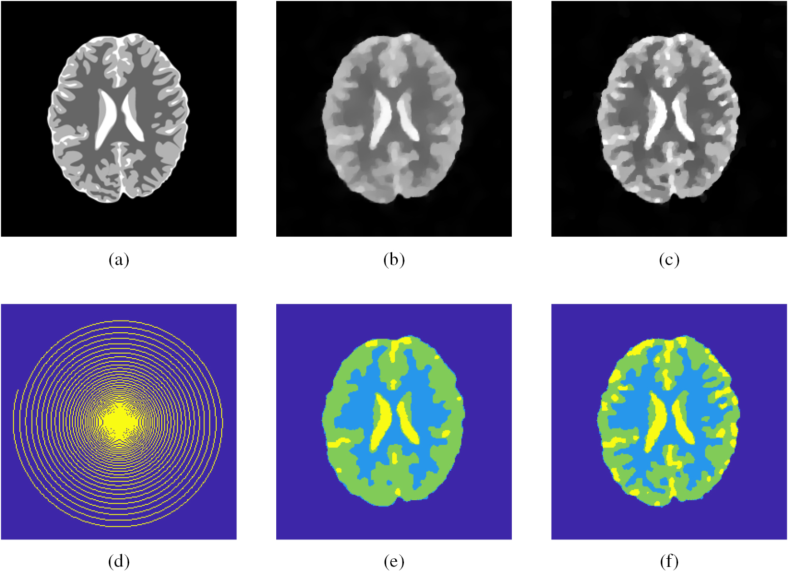
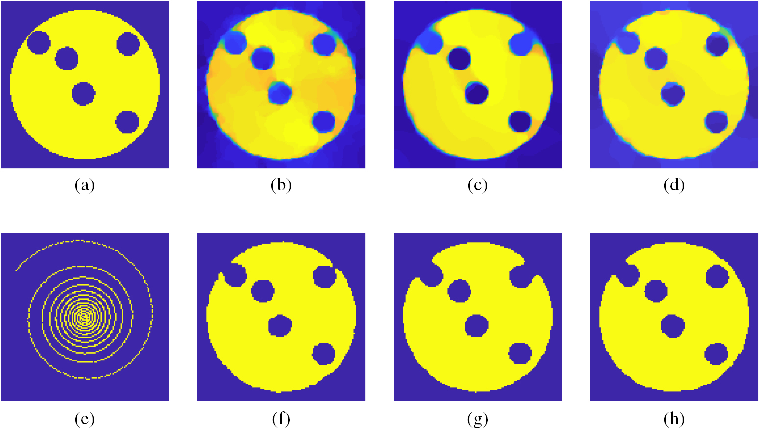
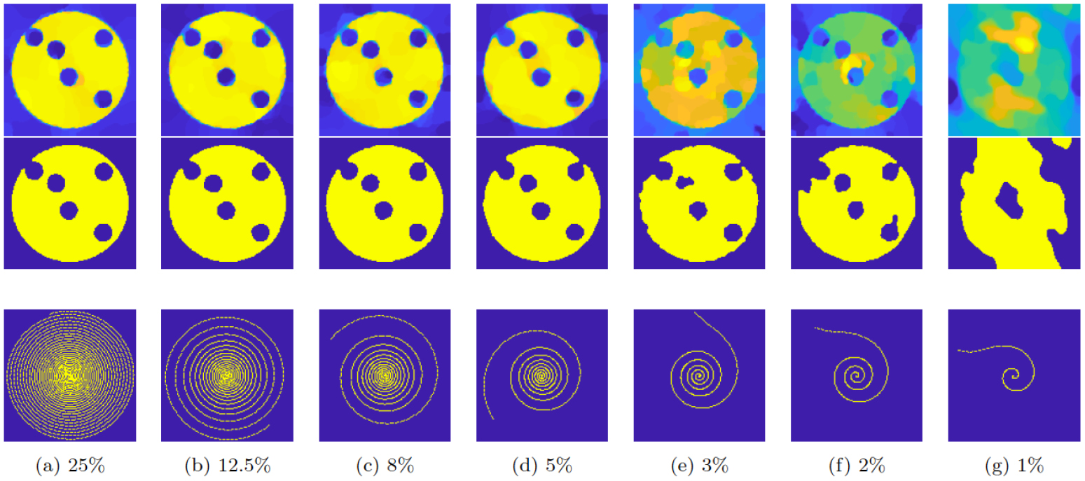
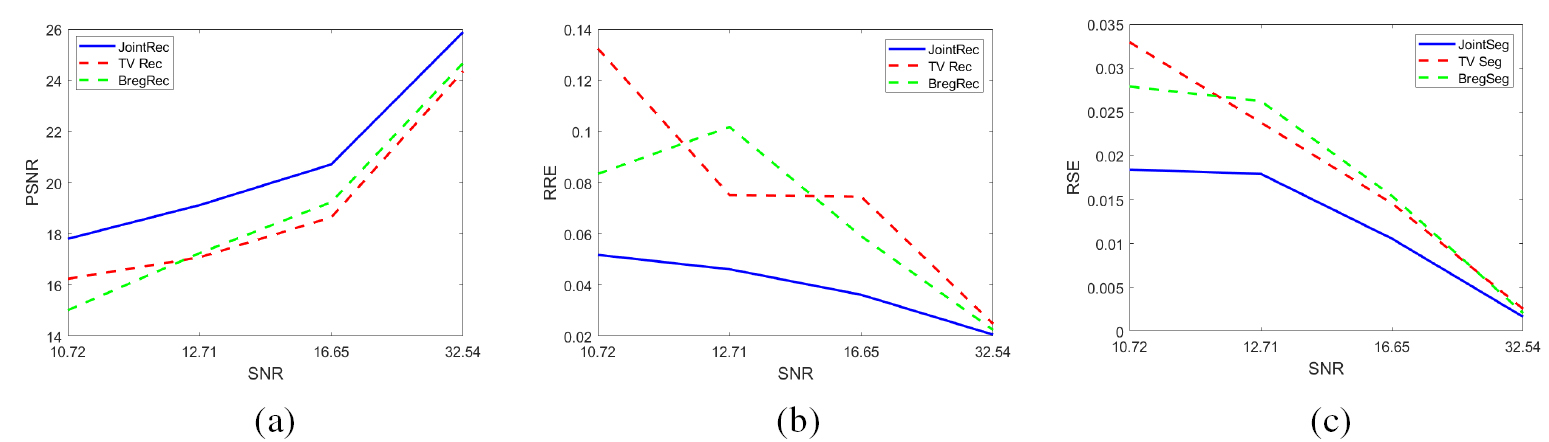
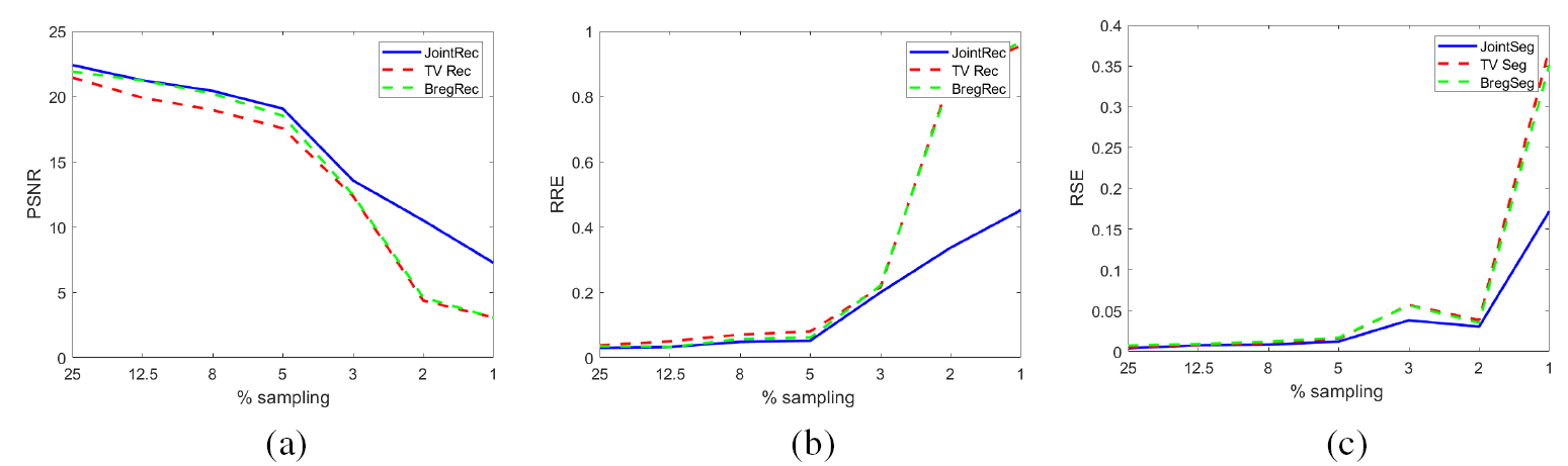
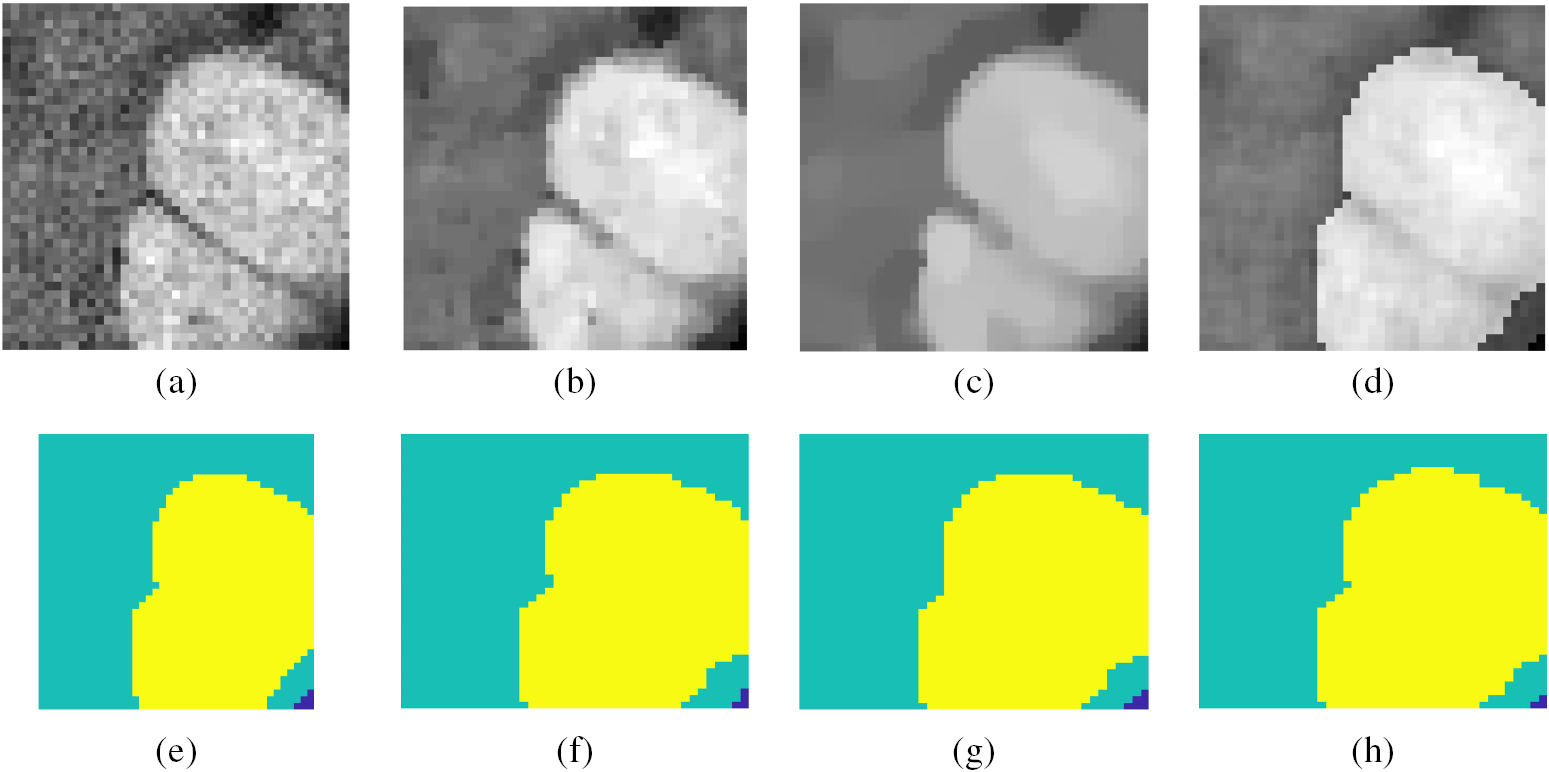
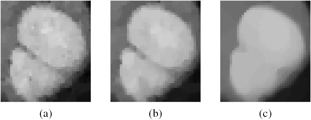
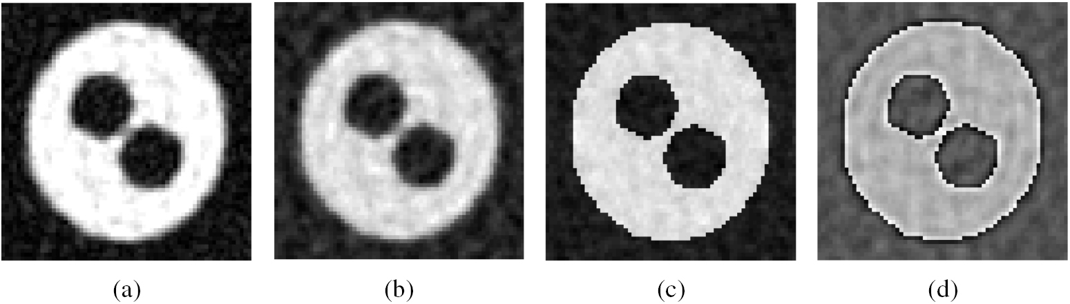
Figure A3. In this example for the bubbly flow, we can see clearly an improvement for both joint reconstruction and joint segmentation. The contrast in the joint reconstruction is better recovered and the segmentation is more accurate, especially for the bubbles close to the edge of the pipe. The joint method results particularly useful for the bubbly flow application. (a) Groundtruth. (b) TV reconstruction,  , RRE = 0.074, PSNR = 17.15. (c) Bregman reconstruction,
  , RRE = 0.071, PSNR = 17.65. (d) Joint reconstruction,
  , RRE = 0.047, PSNR = 19.015. (e) Sampling matrix, 8%. (f) Segmentation,
  , RSE = 0.016. (g) Bregman segmentation,
  , RSE = 0.022. (h) Joint segmentation,
  ,
,  , RSE = 0.014.
Download figure:
Standard image High-resolution image