


Abstract
Particle image velocimetry (PIV) has become the chief experimental technique for velocity field measurements in fluid flows. The technique yields quantitative visualizations of the instantaneous flow patterns, which are typically used to support the development of phenomenological models for complex flows or for validation of numerical simulations. However, due to the complex relationship between measurement errors and experimental parameters, the quantification of the PIV uncertainty is far from being a trivial task and has often relied upon subjective considerations. Recognizing the importance of methodologies for the objective and reliable uncertainty quantification (UQ) of experimental data, several PIV-UQ approaches have been proposed in recent years that aim at the determination of objective uncertainty bounds in PIV measurements.
This topical review on PIV uncertainty quantification aims to provide the reader with an overview of error sources in PIV measurements and to inform them of the most up-to-date approaches for PIV uncertainty quantification and propagation. The paper first introduces the general definitions and classifications of measurement errors and uncertainties, following the guidelines of the International Organization for Standards (ISO) and of renowned books on the topic. Details on the main PIV error sources are given, considering the entire measurement chain from timing and synchronization of the data acquisition system, to illumination, mechanical properties of the tracer particles, imaging of those, analysis of the particle motion, data validation and reduction. The focus is on planar PIV experiments for the measurement of two- or three-component velocity fields.
Approaches for the quantification of the uncertainty of PIV data are discussed. Those are divided into a-priori UQ approaches, which provide a general figure for the uncertainty of PIV measurements, and a-posteriori UQ approaches, which are data-based and aim at quantifying the uncertainty of specific sets of data. The findings of a-priori PIV-UQ based on theoretical modelling of the measurement chain as well as on numerical or experimental assessments are discussed. The most up-to-date approaches for a-posteriori PIV-UQ are introduced, highlighting their capabilities and limitations.
As many PIV experiments aim at determining flow properties derived from the velocity fields (e.g. vorticity, time-average velocity, Reynolds stresses, pressure), the topic of PIV uncertainty propagation is tackled considering the recent investigations based on Taylor series and Monte Carlo methods. Finally, the uncertainty quantification of 3D velocity measurements by volumetric approaches (tomographic PIV and Lagrangian particle tracking) is discussed.
Export citation and abstract BibTeX RIS

Original content from this work may be used under the terms of the Creative Commons Attribution 3.0 licence. Any further distribution of this work must maintain attribution to the author(s) and the title of the work, journal citation and DOI.
1. Introduction
1.1. Relevance of uncertainty quantification in particle image velocimetry (PIV)
PIV has undergone great advances over the past 30 years, becoming the leading flow measurement technique for research and development in fluid mechanics (Adrian 2005. Adrian and Westerweel 2011, Raffel et al 2018). Thanks to its versatility and ability to reveal the 3D structures in complex flow fields, applications of PIV have been reported for a wide range of flow regimes and length scales, from creeping flows (velocities of the order of 1 mm s−1, Santiago et al 1998) to supersonic and hypersonic flows (velocities of the order of 1000 m s−1, Scarano 2008, Avallone et al 2016), from nanoscale flow phenomena (Stone et al 2002) to the dynamics of the atmosphere of Jupiter (Tokumaru and Dimotakis 1995). The use of PIV is very attractive also for aerodynamic research and development in industrial facilities, where it enables understanding complex flow phenomena such as those in separated flows over aircraft models in high-lift configuration, or vortices behind airplanes, propellers or rotors (Kompenhans et al 2001). Furthermore, PIV provides adequate experimental data for the validation of numerical simulations, so to determine whether the physics of the problem has been modelled correctly (Ford et al 2008, de Bonis et al 2012).
Nevertheless, PIV measurements are not and will never be perfect. Uncertainty quantification (UQ) offers a rational basis to interpret the scatter on repeated observations, thus providing the means to quantify the measurement inaccuracies and imprecisions (Kline 1985, Moffat 1988). Uncertainty analysis in PIV experiments can be used for several purposes.
- (a)During the phase of experimental design, to select which instrumentation (e.g. cameras, laser, tracer particles) and experimental parameters (e.g. seeding concentration, optical setup, light source pulse separation time) maximize the measurement accuracy for a given experiment. Also, it allows avoiding 'hopeless' experiments, where the desired accuracy requirements cannot be met with the available instrumentation.
- (b)During the phase of image evaluation, it supports the selection of the appropriate processing parameters (e.g. correlation algorithm, interrogation window size and shape) that maximize the quality of the results (Foucaut et al 2004).
- (c)For physical discovery experiments, designed and conducted to increase the fundamental understanding of some physical process, it enables avoiding misinterpretation of the results. By knowing the uncertainty bounds, the experimenter knows which physical phenomena are indeed captured by the experiment, and which instead are purely an artefact of the measurement system. The estimated uncertainty can also be employed to reduce measurement errors by suppressing the random noise, while preserving true flow fluctuations (Wieneke 2017a).
- (d)For model calibration experiments, carried out to construct, improve or determine parameters in physical models (e.g. calibration of turbulence model parameters), it enables to determine the range of acceptable parameters.
- (e)For validation benchmark experiments, executed to determine the ability of a mathematical model to predict a physical process (Smith 2016), uncertainty quantification provides the only appropriate basis for deciding whether numerical simulations agree with experimental data within acceptable limits, and whether results on one phenomenon from two or more laboratories agree or disagree.
- (f)For data assimilation approaches, where PIV measurements are combined with CFD simulations to determine flow quantities otherwise inaccessible or difficult to measure, knowledge of the PIV measurement uncertainty is crucial to adequately condition the numerical simulations based on the local uncertainty of the PIV data (Symon et al 2017).
A typical figure for the uncertainty of PIV displacements is reported as 0.1 pixel units (Adrian and Westerweel 2011). However, the use of such 'universal constant' to characterize the uncertainty of PIV measurements is overly simplistic, as the actual uncertainty is known to vary greatly from experiment to experiment, and to vary in space and time even within a single experiment, depending on the specific flow and imaging conditions, and on the image evaluation algorithm. For this reason, in the recent years the PIV community has payed increasing attention to the quantification of the PIV uncertainty, as demonstrated by a dedicated workshop held in Las Vegas in 2011, the constant presence of dedicated sessions at the recent Lisbon International Symposia and the International Symposia on Particle Image Velocimetry, and the increasing number of scientific publications on the topic (figure 1). This work presents a survey of the most relevant approaches for PIV uncertainty quantification, aiming to guide the experimenters in the selection of the right tools and methodologies to evaluate and document the uncertainties of their results.
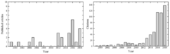
Figure 1. Number of published articles (left) and their citations (right) dealing with PIV uncertainty quantification methodologies (data source: Web of Science).
Download figure:
Standard image High-resolution image1.2. Experimental errors and uncertainty: definitions and classification
Before entering the discussion on PIV measurement errors and uncertainties, general definitions are given following Coleman and Steele (2009) and the Guide to Expression of Uncertainty in Measurement of the International Organization for Standardization (ISO-GUM 2018).
1.2.1. Measurement errors and their classification.
The measurement of a variable X is affected by an error δ, defined as the difference between measured and true value Xtrue:

Since the true value Xtrue is unknown, so is the measurement error. The ISO-GUM classifies the measurement errors into two components, namely random and systematic. Random errors, usually indicated with ε, are due to aleatory processes affecting a measurement; as a consequence, they are unpredictable and typically change their value during a sequence of measurements. By definition, their expected value over repeated measurements is zero. Conversely, systematic (or bias) errors, denoted with β, are fixed or relatively fixed function of their sources (Smith and Oberkampf 2014). Note that, according to the definition embraced by the PIV community, systematic errors are not necessarily constant during a measurement, as they can vary with their input sources. Such definition is counter to that given by Coleman and Steele (2009), who define systematic errors as those which do not vary during the measurement period. All systematic errors of known sign and magnitude can and should be removed. The remaining error is composed by all the random and systematic components that are left unknown:

A representation of their effect on the measurement of X is shown in figure 2.

Figure 2. Representation of random, systematic and total error on a measured variable.
Download figure:
Standard image High-resolution image1.2.2. Measurement uncertainties and their classification.
Because the measurement errors are unknown, the role of UQ is to estimate an interval which contains, with a certain probability, the magnitude of the total error affecting the measured value of X.
To explain the concept of uncertainty, suppose that the measurement of X is repeated N times and that the process is steady, meaning that the true value Xtrue is constant in time. Due to the presence of measurement errors, different measurements yield different outcomes. A distribution of the sample population of the N measurements can be drawn, as illustrated in figure 3, characterized by mean value  and standard deviation sX, respectively. When the number of measurements N approaches infinity, then the sample population distribution approaches the parent population distribution, whose mean µ deviates from Xtrue by β (see figure 3). In presence of solely random errors, β = 0 and the mean value µ of the parent population distribution coincides with the true value Xtrue.

Figure 3. Representation of parent and sample population distribution from repeated measurements.
Download figure:
Standard image High-resolution imageUncertainties are classified into systematic and random, depending on whether they stem from systematic or random error sources, respectively1. Following the ISO-GUM (2018), the random and systematic standard uncertainties are defined as estimates of the standard deviation of the parent population from which an elemental random or systematic error source originates, respectively. They are indicated with sX and bX, respectively. The combined standard uncertainty is obtained from the sum of the squares of the two contributions:
The combined standard uncertainty does not require any assumption on the form of the parent population; hence, the probability that the total error falls within the interval ±uC cannot be determined. For this reason, the expanded uncertainty U is introduced, defined such that

where Xbest is the best estimate of Xtrue, equal to X when a single measurement is conducted, or to  when repeated observations are carried out. The parameter C is called confidence level and is typically set to 95% (Kline and McClintock 1953, Abernethy and Thompson 1973).
The expanded uncertainty is obtained by multiplying the combined standard uncertainty by a coverage factor k:

The determination of the coverage factor requires knowledge of the error distribution. For most engineering and scientific experiments, the error distribution can be assumed Gaussian, and coverage factors of 1, 2 and 3 yield confidence levels of approximately 68%, 95% and 99.7%, respectively.
2. Error sources in PIV measurements
Errors in PIV measurements may be introduced at different phases of the measurement chain, e.g. due to the specific flow facility used, setup of the experimental apparatus, image recording process and choices of the data evaluation methods (figure 4).
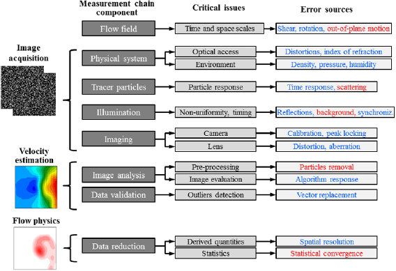
Figure 4. Schematic representations of the main components of the PIV measurement chain and the most relevant error sources. Error sources which are mainly systematic or mainly random are indicated in blue or red, respectively (it should be noted that some error sources such as peak locking are both random and systematic). Reproduced with permission from Wieneke (2017b). © 2017 B.F.A. Wieneke.
Download figure:
Standard image High-resolution imageWieneke (2017b) highlights that, while all error sources are encoded in the recorded images (except those due to sub-optimal image processing), some of them remain 'hidden' and their uncertainty cannot be quantified by analyzing the image recordings. Those error sources, typically systematic in nature, include tracer particle response, hardware timing and synchronization, perspective errors and calibration errors (especially for stereo-PIV and tomo-PIV). Instead, the uncertainty associated with error sources such as particle image size and shape, camera noise, seeding density, illumination intensity variation, particle motion and image interrogation algorithm can be quantified from the image recordings via the UQ methods that will be explained in section 3. Following Raffel et al (2018), PIV measurement errors can be broadly categorized into errors caused by system components, due to the flow itself and caused by the evaluation technique. For an in-depth discussion on PIV error sources, the interested reader is referred to the textbooks of Adrian and Westerweel (2011) and Raffel et al (2018).
It should be remarked that, whenever possible, the experimenter should use a-priori information on the PIV uncertainty to design and conduct the experiment in such a way that measurement errors are avoided or minimized. Since not all errors can be avoided or reduced below a minimum level, the experimenter should use a-posteriori uncertainty quantification tools to quantify the uncertainty associated with the most relevant remaining error sources.
2.1. Errors caused by system components
2.1.1. Errors due to installation and alignment.
Planar (2D2C) PIV systems measure the projection of the flow velocity vector onto the measurement plane. If the measurement plane is not properly aligned with the desired flow direction, the velocity projection does not correspond to the flow components of interest, thus yielding systematic errors (Raffel et al 2018). Additionally, in presence of an out-of-plane velocity component, perspective errors are produced whose magnitude increases linearly with the distance from the optical axis of the camera lens. Such errors can be attenuated or avoided by increasing the distance between lens plane and measurement plane, using telecentric lenses (Konrath and Schöder 2002) or adding a second camera in stereoscopic configuration (Prasad 2000). Furthermore, errors are introduced in the calibration procedure if the calibration plate has not been manufactured accurately, or if the calibration plane does not coincide exactly with the measurement plane. In stereoscopic and tomographic PIV measurements, the latter errors can be corrected for via self-calibration approaches (Wieneke 2005, 2008). Additional calibration errors arise when the measurements are conducted with a relatively thick laser sheet and the optical magnification varies along the direction of the optical axis, yielding erroneous velocity estimates depending on the depth position of the tracer particles (Raffel et al 2018).
2.1.2. Timing and synchronization errors.
The pulse delay Δt of the light source may differ from the value selected by the user. Possible causes vary from the complex physics associated with the lasing process and successive release of the laser energy (Bardet et al 2013), to the use of different cable lengths employed to trigger the system components (Raffel et al 2018). Since in PIV the flow velocity is computed from the ratio between particles displacement and pulse delay Δt, an error on the latter has direct consequences on the uncertainty of the velocity measurements.
Bardet et al (2013) conducted a thorough investigation on the timing issues of a wide range of commercially available Q-switched Nd:YAG and Nd:YLF lasers. The timing errors of all tested lasers were found to be mainly systematic, whereas the random errors were negligible. Systematic errors of up to 50 ns, 1.5 µs and several microseconds were measured for Nd:YAG, dual-cavity Nd:YLF, and single-cavity Nd:YLF lasers, respectively. While these timing errors may be considered negligible for measurements in low-speed flows, where the typical pulse delay is of the order of 100 µs or larger, they become critical for flow measurements in microfluidics and supersonic or hypersonic regimes, where a pulse delay of the order of 1 µs or lower is required. However, since these errors are mainly systematic in nature, they can be easily corrected electronically. Furthermore, in supersonic flows, the finite laser pulse width (of the order of 10 ns) may cause particle images streaks elongated in the flow direction, thus resulting in additional measurement errors (Ganapathisubramani and Clemens 2006).
2.1.3. Particles tracing capability.
The velocity of a tracer particle is, in general, different from that of the surrounding fluid; the difference between the two velocities is defined as particle slip velocity. In the assumption that the particle's motion is governed by Stoke's drag law, the slip velocity depends on the local fluid acceleration and the particle time response, where the latter is proportional to the square of the particle diameter and to the density difference between particle and fluid (Mei 1996, Raffel et al 2018). For air flows, liquid or solid tracer particles are usually employed, which are typically much heavier than air. To enable good tracing capabilities, the particle diameter is selected in the range 0.01–2 µm (Melling 1997, Wang et al 2007, Ghaemi et al 2010, Ragni et al 2011). The recent introduction of neutrally-buoyant helium-filled soap bubbles has enabled increasing the particle diameter to about 300–500 µm, while maintaining a particle time response of the order of 10 µs (Bosbach et al 2009, Scarano et al 2015, Faleiros et al 2018).
In liquid flows, achieving the condition of good tracers is much easier due to the higher density and viscosity of the fluid, and the fact that the experiments are typically conducted at lower speeds. Hence, low response time can be still achieved with tracer particles of 10–50 µm diameter (Melling 1997).
2.1.4. Imaging.
Peak-locking is possibly the error that has received the largest attention in digital PIV (Westerweel 1997a, Christensen 2004, Overmars et al 2010, among many others). It occurs mainly when the particle image is small compared to the pixel size (particle image diameter not exceeding one pixel) and has the effect of biasing the measured particle image displacement towards the closest integer pixel value. As a result, the measured velocity may be overestimated or underestimated depending on the sub-pixel length of the particle image displacement. The magnitude of peak locking errors varies considerably with the algorithm used to fit the cross-correlation displacement peak (Roesgen 2003). This source alone can produce errors of the order of 0.1 pixels, which have a great impact on the accuracy of turbulence statistics (Christensen 2004). Several approaches have been proposed for the minimization or correction of peak-locking errors, including use of a smaller optical aperture, optical diffusers (Michaelis et al 2016, Kislaya and Sciacchitano 2018), image defocusing (Overmars et al 2010), multi-Δt image acquisition (Nogueira et al 2009, 2011, Legrand et al 2012, 2018) and data post-processing approaches (Roth and Katz 2001, Hearst and Ganapathisubramani 2015, Michaelis et al 2016).
Additional errors associated with the imaging of the tracer particles are ascribed to the noise in each pixel reading. Image noise affects the accuracy to which a particle image displacement can be measured by the image analysis algorithm. Digital cameras have mainly three types of noise sources, namely background (dark) noise, photon shot noise and device noise (Adrian and Westerweel 2011). For a detailed comparison of the performances of different sensors typically employed in digital PIV (namely CCD, CMOS and intensified CMOS sensors), the reader is referred to the work of Hain et al (2007).
2.1.5. Illumination.
Measurement errors occur when the two laser pulses are not perfectly aligned with each other, or have different intensity profiles, yielding a variation of the intensity of individual tracer particles (Nobach and Bodenschatz 2009, Nobach 2011). Instead, variations of the illumination intensity between the two laser pulses, or mild spatial variations along the light sheet do not contribute significantly to the measurement error, as the cross-correlation operator is insensitive to absolute intensity variations (Wieneke 2017b). Nevertheless, it is critical that the illumination system delivers sufficient light intensity to ensure enough contrast between the tracer particles and the background (Scharnowski and Kähler 2016a).
2.2. Errors due to the flow
The flow itself may be the cause of measurement errors. Velocity gradients, fluctuations and streamline curvatures may induce errors either due to the particle slip or because of the inability of the image evaluation algorithm to resolve those or cope with them. While the effect of in-plane velocity gradients can be mitigated with state-of-the-art image evaluation algorithms with window deformation (Scarano and Riethmuller 2000), out-of-plane velocity gradients cause errors in the measured in-plane velocity components due to the finite number of particles within an interrogation window and their random positions. Additional measurement errors are ascribed to variations of the fluid properties (e.g. temperature, density, viscosity) or of the flow Reynolds and Mach numbers during the experiment runtime. When the tracer particles move across the light sheet, particles entering or exiting the light sheet lead to unmatched particles that contribute to the background noise in the correlation functions. Furthermore, the change of intensity of overlapping particle images, corresponding to particles at different depths in the measurement plane, leads to random errors in the measured displacement (Nobach and Bodenschatz 2009, Nobach 2011).
At very low velocities (below 1 mm s−1), a random Brownian particle motion becomes visible in high-magnification µPIV measurements. The Brownian motion results in a random in-plane jitter of the particle positions which reduces the signal strength of the correlation function, thus increasing the measurement uncertainty (Olsen and Adrian 2001). The associated measurement error is reported to increase with the fluid temperature, and to decrease with increasing particle diameter and flow velocity (Devasenathipathy et al 2003).
2.3. Errors due to the evaluation technique
Errors associated with the specific evaluation techniques and the selected processing parameters have been analyzed in great detail over the last two decades, as demonstrated by the four international PIV challenges (Stanislas et al 2003, 2005, 2008, Kähler et al 2016). In the early days of PIV, the researchers' attention focused on the problem of detection and removal of wrong vectors (outliers, Keane and Adrian 1990, Westerweel and Scarano 2005). While such problem is relatively simple for isolated outliers, which appear at random locations in the flow field, the detection and removal of clusters of outliers is still a subject of investigation (Masullo and Theunissen 2016). From the end of the 1990s, minimization of the measurement uncertainty and maximization of the spatial resolution have become crucial research topics for the development of PIV algorithms, so to widen the range of resolvable velocity and length scales (dynamic velocity range DVR and dynamic spatial range DSR, respectively, Adrian 1997). For this purpose, researchers have assessed the performances of different evaluation algorithms considering various types of correlation analysis, interrogation window sizes and shapes, cross-correlation peak fit algorithms, image and vector interpolation schemes for image deformation algorithms. The sensitivities of the evaluation algorithms to the most common error sources stemming from flow and imaging conditions have been analyzed, as it will be discussed in detail in section 3.
3. PIV uncertainty quantification approaches
The local flow velocity u at a point (x, y ) is computed by measuring the displacement Δx of a group of tracer particles during a short time interval Δt (Adrian and Westerweel 2011):
M is the magnification factor, which allows converting the displacement Δx in the object space to that in the image plane, indicated with ΔX. The time interval Δt is typically selected much smaller than the characteristic time scale of the flow, so that truncation errors can be neglected. The uncertainty of the estimated velocity is obtained from Taylor series propagation (Coleman and Steele 2009), considering ΔX, Δt and M as independent variables:
The uncertainty UΔt of the laser pulse separation is usually treated as a Type B uncertainty (i.e. it cannot be retrieved from data statistics on repeated observation) and its quantification relies upon information provided by the manufacturer or dedicated experiments (Bardet et al 2013). Typical values of UΔt are of the order of 1 ns (Lazar et al 2010), yielding a negligible relative uncertainty for most experiments (as discussed in section 2.2, such uncertainty may not be negligible for µPIV measurements or experiments in supersonic or hypersonic flow regimes, where a laser pulse separation of 1 µs or smaller may be required). Limited work is reported in literature on the quantification of UM. Gui et al (2001a) estimated the uncertainty of the magnification factor by considering the uncertainties associated with the size of the camera view in the object plane and that of the digital image. Recently, Campagnole dos Santos et al (2018) conducted a more thorough evaluation of the magnification uncertainty, which was calculated as the sum of four contributions, namely (i) the uncertainty of the dot position and size due to the manufacturing limits of the calibration plane; (ii) the image distortion due to perspective errors; (iii) the misalignment between calibration plate and measurement plane; and (iv) the misalignment between calibration plate and camera plane. Additional uncertainty arises from the model form uncertainty of the calibration function (mapping function from image plane to physical space), as the functional form of the latter may not be sufficient to account for all optical distortions. However, when the calibration is conducted properly, the magnification and calibration uncertainties are negligible with respect to the total uncertainty, which is dominated by the displacement term in equation (7). For this reason, much effort has been made in the last decades to quantify the uncertainty of ΔX. The proposed approaches for the quantification of UΔX can be broadly classified into a priori and a posteriori (Sciacchitano et al 2013). The former aim at providing a value or range of UΔX for typical conditions encountered in PIV measurements. Ultimately, a-priori UQ approaches return a general figure for the uncertainty of a PIV algorithm. This is typically done via theoretical modelling of the measurement chain or by assessing the performance of a PIV algorithm based on synthetic images and Monte Carlo simulations. On the other hand, a-posteriori UQ approaches aim at quantifying the local and instantaneous uncertainty of specific sets of data, thus providing the experimenter with uncertainty bands for each measured velocity vector based on the data they acquired.
The most relevant a-priori and a-posteriori PIV UQ approaches are discussed hereafter, highlighting the strengths and limitations of each, and the most important findings about the uncertainty of PIV data and the performances of standard PIV algorithms.
3.1. A-priori uncertainty quantification approaches
A-priori uncertainty quantification for PIV has been proposed since the early days of the technique. Researchers have made use of theoretical modelling of the image analysis algorithm and/or Monte Carlo simulations to determine the typical magnitude of PIV measurement errors and their dependency upon experimental and processing parameters.
3.1.1. A-priori uncertainty quantification by theoretical modelling of the measurement chain.
The earliest attempt to quantify the uncertainty of PIV velocity estimates was made by Adrian (1986), who proposed that the uncertainty of the measured particle image displacement is equal to cdτ, being dτ the particle image diameter and c a parameter associated with the uncertainty in locating the particle image centroid. The particle image diameter dτ can be evaluated either a priori by means of an approximated analytical formula, or a posteriori by computing the auto-correlation function in a certain image domain and then fitting an appropriate functional form to the auto-correlation peak (Adrian and Westerweel 2011). Typical values of c are reported in the order of 0.1. While Adrian's uncertainty principle has the advantage of being extremely easy to implement and apply, the actual value of c depends upon the specific measurement conditions and image analysis algorithm, and remains unknown. Furthermore, Adrian's model does not account for the increase of measurement errors for small particle image size due to peak locking. Moreover, this simple model does not account for error sources stemming from the specific flow conditions (e.g. velocity gradients, out-of-plane motion, streamline curvature) and imaging conditions (e.g. image background noise, laser light reflections, seeding concentration). Finally, recent works have shown that, for particle image diameters exceeding three pixels, the measurement error of state-of-the-art multi-pass interrogation algorithms exhibits little variation when further increasing the particle image diameter (Raffel et al 2018).
Theoretical models have been formulated for the a-priori quantification of the PIV uncertainty. Due to the complexity of the problem, simplifying assumptions for the processing algorithm and flow conditions are made, e.g. cross-correlation-based image analysis with discrete window offset (no image deformation), uniform flow motion, perfect recordings with no image noise or perspective errors. Westerweel (1993, 1997) and Adrian and Westerweel (2011) developed the theoretical framework that describes the working principle of digital PIV in terms of linear system theory. The authors showed that for  , being dr the pixel size, the measurement error is dominated by bias effects due to peak locking, whereas for
  random errors are dominant, which increase proportionally with the particle image diameter. Typical values of minimum measurement errors were reported in the range 0.05 to 0.1 pixels for 32 × 32 pixels interrogation window. Analytical models for the peak locking errors and their effect on turbulence statistics were formulated by Cholemari (2007), Angele and Muhammad-Klingmann (2005) and Legrand et al (2018), among others.
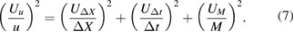
An improved theory for digital image analysis was presented by Westerweel (2000), where an analytical expression was derived that relates the measurement error with the sub-pixel displacement, the particle image diameter and the image density. The theory confirms the results of previous Monte Carlo simulations (Adrian 1991, Willert 1996) that the minimum error occurs for dτ = 2 pixels, and that larger particle image diameters yield increased random errors (figure 5).
Figure 5. RMS error (viz. random uncertainty) as a function of the particle image displacement (left) and diameter (right). Figure reproduced from Westerweel (2000). © Springer-Verlag Berlin Heidelberg (2000). With permission of Springer.
Download figure:
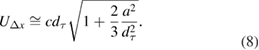
Standard image High-resolution imageThe effect of in-plane velocity gradients in PIV interrogation is addressed in Westerweel (2008), where an analytical expression is derived that describes the amplitude, location and width of the displacement correlation peak in presence of velocity gradients. A correction to Adrian's uncertainty principle is proposed, whereby the effect of the variation of the local particle-image displacement a is included:
It should be remarked that this analysis considers a relatively simple interrogation method with discrete window shift (Westerweel et al 1997). State-of-the-art image interrogation algorithms with window deformation (Scarano and Riethmuller 2000, Fincham and Delerce 2000) are much less prone to errors ascribed to in-plane velocity gradients.
In presence of streamlines curvature, additional bias errors are introduced due to the finite interrogation window size (modulation errors due to spatial filtering; Spencer and Hollis 2005, Lavoie et al 2007). Additionally, by assuming that the particles path is a straight line instead of a curve one, the velocity vector is located at a different streamline than the actual one (Scharnowki and Kähler 2013). By modelling the cross-correlation analysis as a moving-average filter, Scarano (2003) demonstrated that the magnitude of such systematic error is proportional to the second-order spatial derivative of the velocity field and to the interrogation window area. When window weighting is employed such that negative and null frequency responses are avoided, resolving spatial wavelengths smaller than the interrogation window size becomes theoretically possible (Nogueira et al 2005a, 2005b). An analytical formula for the intrinsic response of the cross-correlation operator subject to a sinusoidal displacement of amplitude A was derived by Theunissen (2012), who demonstrated that the cross-correlation operator behaves as a moving-averaged filter only for small ratios A/dτ < 4. The work was further extended by Theunissen and Edwards (2018), who derived a semi-analytical equation for the ensemble average cross-correlation response.
3.1.2. A-priori uncertainty quantification by numerical or experimental assessment.
As discussed in the previous section, theoretical modelling of the measurement chain requires simplifying assumptions for the processing algorithm and the flow and imaging conditions, and does not account for the full complexity of the experimental setup and image analysis. For this reason, much research has been conducted to quantify a priori the measurement uncertainty either via synthetic images and Monte Carlo simulations, or by experimental assessment. In the former case, images are generated with a random distribution of tracer particles which follow a prescribed motion. In this respect, the works of Okamoto (2000) and Lecordier and Westerweel (2004) define the guidelines for the selection of key parameters for standard PIV images, e.g. particle image diameter, shape and intensity, seeding concentration and laser sheet thickness and shape. The use of synthetic images yields some major advantages (Scharnowski and Kähler 2016b): (a) the true velocity field is known, from which the evaluation of the actual measurement error is straightforward; (b) total control of all experimental parameters (e.g. particle image size, concentration, turbulence intensity, etc), which can be changed individually without modifying the others; (c) possibility to set those parameters to values that are not easily achievable in real experiments (e.g. extremely low or high turbulence levels); and (d) ease and rapidity of implementation, since no wind tunnel or equipment is required to generate synthetic images. Due to these advantages, the use of synthetic images and Monte Carlo simulations has become a standard approach for evaluating the performances of PIV analysis methods, and the uncertainty associated with imaging, flow and processing parameters. Bias and random errors have been characterized for different PIV algorithms (e.g. single-pass correlation, discrete and sub-pixel window shift, window deformation) as a function of parameters such as particle image size and displacement, displacement gradient, seeding concentration, out-of-plane particle motion, image interpolation algorithm, cross-correlation peak fit algorithm. A selection of representative investigations where a-priori UQ analyses is carried out via synthetic images and Monte Carlo simulations is reported in table 1.
Table 1. List of error sources investigated by Monte Carlo simulations and selection of references where such investigations are conducted.
| Error sources investigated | References |
|---|---|
| Particles motion (displacement, displacement gradient, out-of-plane motion) | Keane and Adrian (1990), Fincham and Spedding (1997), Scarano and Riethmuller (1999), Fincham and Delerce (2000), Wereley and Meinhart (2001), Mayer (2002), Stanislas et al (2003), Foucaut et al (2004), Nobach and Bodenschatz (2009), Scharnowski and Kähler (2016b) |
| Imaging conditions (particle image diameter, seeding density, camera noise, sensor fill factor) | Willert and Gharib (1991), Willert (1996), Fincham and Spedding (1997), Stanislas et al (2003), Foucaut et al (2004), Duncan et al (2009), Scharnowski and Kähler (2016a, 2016b) |
| Interrogation window size and weighting function | Gui et al (2001b), Lecordier et al (2001), Nogueira et al (2005b), Duncan et al (2009), Eckstein and Vlachos (2009) |
| Image interrogation algorithm | Huang et al (1997), Scarano and Riethmuller (2000), Lecordier et al (2001), Meunier and Leweke (2003), Stanislas et al (2003, 2005, 2008), Foucaut et al (2004) |
| Peak locking | Nogueira et al (2001), Gui and Wereley (2002), Fore (2010), Michaelis et al (2016) |
| Spatial resolution | Astarita (2007), Nogueira et al (1999, 2002), Stanislas et al (2003, 2005, 2008), Elsinga and Westerweel (2011), Kähler et al (2012a, 2012b, 2016) |
| Image interpolation scheme for multi-pass image deformation methods | Astarita and Cardone (2005), Nobach et al (2005), Astarita (2006), Kim and Sung (2006), Duncan et al (2009) |
| Vector interpolation scheme for multi-pass image deformation methods | Astarita (2008) |
Most of the investigations conducted via Monte Carlo simulations agree that a typical figure for the error magnitude is in the range 0.01–0.2 pixels depending on the simulated flow and imaging conditions and on the processing algorithm employed. In particular, it has been shown that multi-pass interrogation algorithms employing image deformation yield the minimum measurement errors. Nevertheless, it is widely acknowledged that synthetic images yield unrealistically low measurement errors due to the assumption of overly-idealized imaging and flow conditions (Stanislas et al 2005). For this reason, a number of works proposed experimental assessments as a valuable alternative to Monte Carlo simulations, aiming to reproduce with a higher degree of realism the complexities and imperfections of actual PIV measurements. In such assessments, the measurement error is computed via direct comparison between measured and exact velocity field, where the latter is either imposed or quantified via a more accurate measurement system. A special case is that of µPIV, where the low Reynolds numbers enable making use of numerical flow simulations to assess the measurement uncertainty (Cierpka et al 2012). A selection of representative a-priori UQ analyses conducted by experimental assessment is reported in table 2.
Table 2. Selection of representative a-priori uncertainty quantification analysis conducted by experimental assessment.
| Experimental assessment method | Error sources investigated | References |
|---|---|---|
| Flow measurement with null or uniform displacement (actual or produced by electro-optical image shifting) | Interrogation algorithm | Willert (1996), Forliti et al (2000) |
| Imaging conditions | Willert (1996), Reuss et al (2002), Scharnowski and Kähler (2016b) | |
| Out-of-plane particle motion | Scharnowski and Kähler (2016a) | |
| Speckle pattern undergoing prescribed motion (translation and/or rotation) | Interrogation algorithm | Prasad et al (1992), Lourenço and Krothapalli (1995) |
| Imaging conditions | Willert and Gharib (1991) | |
| Out-of-plane particle motion | Nobach and Bodenschatz (2009) | |
| Particle motion and background noise in tomographic PIV | Liu et al (2018) | |
| Comparison with more accurate measurement system | Spatial resolution | Spencer and Hollis (2005), Lavoie et al (2007) |
| Peak locking | Kislaya and Sciacchitano (2018) | |
| Comparison between unconverged and converged statistics | Precision uncertainty in statistical properties | Carr et al (2009) |
| Comparison among different processing algorithm | Peak locking | Christensen (2004), Kähler et al (2016) |
| Particle displacement and displacement gradient | Stanislas et al (2003) |
From the experimental assessments, it emerges that PIV displacement errors can be as large as several tenths of a pixel, especially in presence of severe out-of-plane motion and peak locking, under-resolved length scales and low image quality. Furthermore, as concluded from the analysis of case B of the 4th International PIV Challenge (Kähler et al 2016), the human factor plays a key role in the overall quality of the measured velocity field, because the selection of the evaluation parameters is often based not only on best practices reported in literature, but also on personal experience.
3.2. A-posteriori uncertainty quantification approaches.
As discussed above, measurement errors in PIV depend upon several factors of the flow characteristics, experimental setup and image processing algorithm. Most of these factors vary in space and time, leading to non-uniform errors and uncertainties throughout the flow fields. The aim of a-posteriori uncertainty quantification is to quantify the local instantaneous uncertainty of each velocity vector. For this purpose, several a-posteriori UQ approaches have been proposed over the last decade. These approaches are typically classified (Bhattacharya et al 2018) into indirect methods, which make use of pre-calculated information obtained by calibration, and direct methods, which instead extract the measurement uncertainty directly from the image plane using the estimated displacement as prior information. As these approaches rely upon different principles, each of them has its own peculiarities in terms of performances and limitations, which are discussed hereafter and summarized in table 4.
3.2.1. Indirect methods.
3.2.1.1. Uncertainty surface method.
The uncertainty surface method (Timmins et al 2012) was the first a-posteriori uncertainty quantification approach that aimed at quantifying the local instantaneous uncertainty of each velocity vector. The method requires the identification of the sources that have the largest contribution to the PIV measurement errors. Timmins et al considered four main contributors, namely particle image diameter, seeding density, shear rate and particle image displacement. In principle, also other error sources such as magnification and calibration errors, streamlines curvature, image noise and out-of-plane particles motion (evaluated by adding a stereoscopic camera or via analysis of the cross-correlation function, Scharnowski and Kähler 2016b) could be accounted for.
After the chief error sources have been identified, synthetic images are generated where the values of the error sources are varied within ranges of typical PIV experiments. The images are then analysed via the PIV processing algorithm, and the resulting velocity fields are compared with the known true velocities to determine the distributions of the measurement errors as a function of each of the error source parameters. This process is illustrated in the top row of figure 6. The distribution of the measurement errors is used to determine a 95% confidence interval that contains the true displacement. The upper and lower random uncertainty bounds (denoted as rhigh and rlow, respectively) are computed in such a way that the probability of displacements  and
and  are both 2.5%, being
  the mean measured displacement for the specific combination of error sources. As a consequence, the random error is contained within the range [−rlow, +rhigh] with a probability of 95%. The systematic uncertainty bk is evaluated from the difference between
  and the known true displacement ΔXtrue, yielding the combined uncertainty estimates:

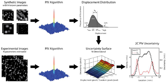
Figure 6. Schematic representation of the working principle of the uncertainty surface method. Reproduced with permission (courtesy of S.O. Warner)
Download figure:
Standard image High-resolution imageThis procedure is conducted for both velocity components of the planar PIV measurement, yielding different uncertainty bounds for the horizontal and vertical displacements. When the analysis above is repeated for all possible combinations of the N error sources, an N-dimensional uncertainty surface is built, which relates the uncertainty bounds with each combination of the N selected error sources.
After the uncertainty surface has been built from the synthetic images, the experimental images are scrutinized. The analysis of the latter yields the local and instantaneous values of the error sources (e.g. displacement, shear, particle image diameter and seeding density), which are given as input to the uncertainty surface to determine the lower and upper uncertainty bounds of each component of each velocity vector (bottom row of figure 6).
The uncertainty surface method has the clear benefit that it provides the (asymmetric) distributions of the measurement errors without requiring any assumption on the shape of those. Furthermore, it can distinguish random and systematic uncertainty components. However, the method relies on the selection of the error sources, and on the evaluation of the values of each error source, which are themselves affected by measurement uncertainty. Additionally, the computation of the uncertainty surface is rather time consuming. Moreover, being uncertainty surface algorithm-dependent, a new uncertainty surface should be built every time a parameter in the image evaluation algorithm is modified.
3.2.1.2. Cross-correlation signal-to-noise ratio metrics.
Approaches based on the cross-correlation signal-to-noise ratio metrics estimate the measurement uncertainty only from quantities derived from the cross-correlation plane, without requiring any assumption, selection or evaluation of the individual error sources. The basic principle is that, for correlation-based image evaluation, the error of the estimated particle image displacement is related to a relevant metrics ϕ representative of the signal-to-noise ratio (SNR) of the cross-correlation function.
Based on the analysis of synthetic images, where the true displacement field is known and the actual measurement error can be directly computed, Charonko and Vlachos (2013) and Xue et al (2014) proposed the following empirical relationship between the standard uncertainty of the measured displacement magnitude  and a generic cross-correlation SNR metrics ϕ:
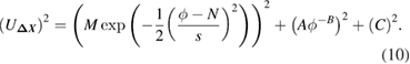
Equation (10) shows how the measurement uncertainty is evaluated as the sum of three contributions. The first term is a Gaussian function employed to account for the uncertainty due to outliers, which typically occur at low values of the correlation SNR (ϕ approaching N, being N the theoretical minimum value of the calculated metrics). The parameter M represents the uncertainty associated with outliers or invalid vectors, defined as vectors for which the difference between measured displacement and true displacement is larger than half of the cross-correlation peak diameter. The parameter s governs how quickly the uncertainty climbs to M for decreasing ϕ values. The second term is a power law that represents the contribution of the valid vectors to the measurement uncertainty. The exponent B > 0 indicates that the higher the correlation signal-to-noise ratio, the lower the measurement uncertainty. In absence of outliers (M = 0), the largest uncertainty is obtained for ϕ approaching its theoretical minimum value N, and is governed primarily by A. The last constant term indicates the lowest achievable uncertainty, which is equal to the parameter C.
Different metrics for the evaluation of the cross-correlation signal-to-noise ratio have been proposed in literature, which are summarized in table 3.
Table 3. Definition of different metrics for the cross-correlation signal-to-noise ratio.
| Metrics | Definition | Reference |
|---|---|---|
| Cross-correlation primary peak ratio PPR (see figure 7 top) | Ratio between largest correlation peak Cmax and second highest correlation peak C2: | Charonko and Vlachos (2013) |
 |
||
| Peak to root-mean-square ratio PRMSR (see figure 7 bottom-left): | Ratio between the square of the primary peak height and the mean-square of the cross-correlation values in the noise part of the correlation plane: | Xue et al (2014) |
 |
||
| Peak to correlation energy PCE (see figure 7 bottom-right) | Ratio between the square of the primary peak height and the correlation energy (mean-square of the cross-correlation values in the entire correlation plane): | Xue et al (2014) |
 |
||
| Inverse of the cross-correlation entropy | ![${{\left({\rm Entropy} \right)}^{-1}}=-{{\left[\sum\nolimits_{i=1}^{{{N}_{{\rm bin}}}}{{{p}_{i}}\log}\left({{p}_{i}} \right) \right]}^{-1}}$](https://content.cld.iop.org/journals/0957-0233/30/9/092001/revision2/mstab1db8ieqn013.gif) with with  |
Xue et al (2014) |
| Mutual information MI | Ratio between largest correlation peak Cmax and height A0 of the auto-correlation of the average particle image: | Xue et al (2015) |
 |
||
| Loss of Particle Ratio LPR | Correction to the MI metrics to account also for the unmatched particle images: | Novotny et al (2018) |
 |
||
| with NI image density and dx the particle image displacement. |
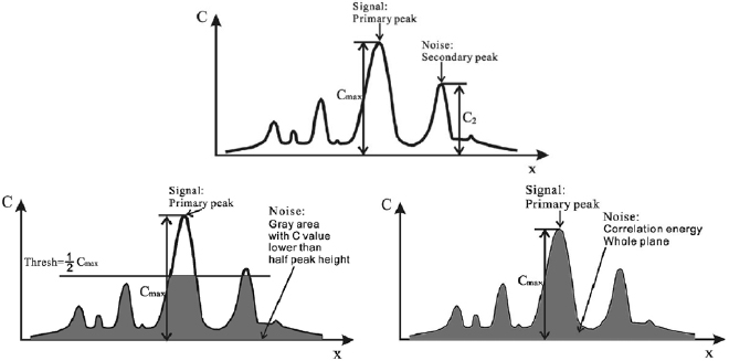
Figure 7. Graphical representation of a 1D cross-correlation function. Top: PPR; bottom-left: PRMSR; bottom-right: PCE. Reproduced from Xue et al (2014). © IOP Publishing Ltd. All rights reserved.
Download figure:
Standard image High-resolution imageTable 4. Main advantages and drawbacks of the a-posteriori PIV uncertainty quantification approaches.
| PIV-UQ Method | Type | Advantages | Drawbacks |
|---|---|---|---|
| Uncertainty surface (Timmins et al 2012) | Indirect | • No hypothesis on the shape of the error distribution | • The approach relies upon estimates of the values of the error sources, which are themselves affected by uncertainty |
| • Able to distinguish upper and lower uncertainty band limits | • Flow unsteadiness, turbulence and unresolved length scales not accounted for | ||
| • Able to distinguish systematic and random uncertainty components | • Need to re-generate the uncertainty surface if any processing parameter is modified | ||
| • Able to quantify uncertainty associated with peak locking errors | • Large computational time to generate the uncertainty surface | ||
| Cross-correlation signal-to-noise ratio metrics (Charonko and Vlachos 2013, Xue et al 2014, 2015, Novotny et al 2018) | Indirect | • Makes use solely of the information contained in the calculated correlation plane | • Provides only the uncertainty of the displacement magnitude, and not that of the individual displacement components |
| • Easy implementation | • Relies upon an empirically developed model | ||
| • Negligible additional computational cost | |||
| • It can in principle quantify the uncertainty associated with outliers | |||
| Particle disparity (Sciacchitano et al 2013) | Direct | • No assumption required on flow and imaging conditions | • Relies upon the identification of the location of the particle images, which may be affected by uncertainty |
| • Provides the (standard) uncertainty of each velocity component | • Intrinsic variability of the uncertainty estimate of about 5%–25% due to the finite number of particle images contained within the interrogation window | ||
| • Provides both the systematic and random components of the uncertainty | • Unable to detect outliers and quantify the uncertainty associated with those | ||
| • Inaccurate in presence of peak locking | |||
| Correlation statistics (Wieneke 2015) | Direct | • No assumption required on flow and imaging conditions | • Intrinsic variability of the uncertainty estimate of about 5%–25% due to the finite number of particle images contained within the interrogation window |
| • Provides the (standard) uncertainty of each velocity component | • Unable to detect outliers and quantify the uncertainty associated with those | ||
| • Does not require the identification and location of particle images | • Peak locking errors remain undetected | ||
| Moment of correlation (Bhattacharya et al 2018) | Direct | • Solely information contained in the calculated correlation plane is used | • The uncertainty estimate is affected by truncation errors due to the discrete nature of the cross-correlation function |
| • Easy implementation | |||
| • Negligible additional computational cost | |||
| Error sampling (Smith and Oberkampf 2014) | Direct | • Accounts for the uncertainty associated with the entire measurement apparatus (facility and equipment, not only the image evaluation process) |
|
| • Allows to quantify the uncertainty associated with time-varying systematic errors | |||
Overall, the uncertainty quantification methods based on the cross-correlation signal-to-noise metrics are extremely simple to implement and apply, and fully rely on the information contained in the cross-correlation plane, without requiring any evaluation of the magnitude of the error sources. However, it should be noticed that these approaches provide the uncertainty of the displacement magnitude, from which the uncertainty of the individual displacement components can be retrieved under certain assumptions (e.g. isotropic errors). Furthermore, they rely upon an empirically developed model, where six parameters must be determined based on fitting with synthetic data.
3.2.2. Direct methods.
3.2.2.1. Particle disparity method.
In the particle disparity or image matching method (Sciacchitano et al 2013), the standard uncertainty of the measured particle image displacement is quantified considering the contribution of individual particle images to the cross-correlation peak. The basic idea is that, in case of perfect match among particle images of an image pair, the cross-correlation function features a sharp correlation peak, whose width is proportional to the particle image diameter; in this case, the measurement uncertainty is the minimum. Conversely, when the particle images do not match perfectly, a residual positional disparity is present, which has the effect of broadening the cross-correlation peak and in turn yield higher uncertainty of the measured displacement. The approach matches the particle images of two corresponding interrogation windows at the best of the velocity estimator, and computes a positional disparity between matched particles (figure 8(left)): statistical analysis of the disparity ensembles yields the estimated measurement uncertainty (figure 8(right)).
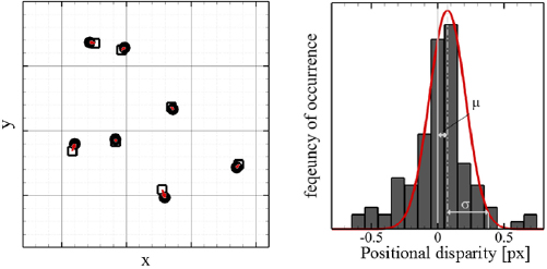
Figure 8. Illustration of the positional disparity between paired particle images (left) and their distribution (right; a larger interrogation window is used for sake of statistical convergence). Figure readapted from Sciacchitano et al (2013). © IOP Publishing Ltd. All rights reserved.
Download figure:
Standard image High-resolution imageThe method provides the (standard) uncertainty of each velocity component without requiring any assumption on the flow and imaging conditions. However, it relies upon the identification and location of individual tracer particle images, where the latter is affected by measurement uncertainty especially in presence of overlapping particle images or poor imaging conditions. Furthermore, the estimated uncertainty features an intrinsic variability of (2NI)−1/2 (typically 5%–25% of the estimate value), where NI is the image density (Keane and Adrian 1990).
3.2.2.2. Correlation statistics method.
The correlation statistics method (Wieneke 2015) is an extension of the particle disparity method where the uncertainty is quantified from the analysis of individual pixels of the images and of their contribution to the cross-correlation peak. The method relies on the assumption that an iterative multi-pass PIV algorithm with window deformation (Scarano 2002) and predictor-corrector filtering (Schrijer and Scarano 2008) is employed for the image analysis, and that the algorithm has reached convergence. In the latter case, the primary peak of the cross-correlation function is symmetric. This is true even in presence of error sources: the predictor-corrector scheme compensates for those error sources, returning a symmetric correlation peak, from which the measured displacement ΔXmeas is evaluated. Hence, the true (unknown) displacement ΔXtrue is associated with an asymmetric correlation peak, whose asymmetry is governed by the (unknown) measurement error δ = ΔXmeas − ΔXtrue. The correlation statistics method evaluates the contribution of each pixel to the asymmetry of the correlation peak, and associates such asymmetry with the uncertainty of the measured displacement (figure 9).
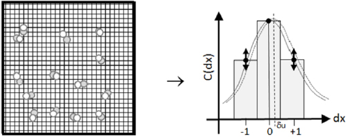
Figure 9. Illustration of the working principle of the correlation statistics method. Image reproduced from Wieneke (2015). © IOP Publishing Ltd. CC BY 3.0.
Download figure:
Standard image High-resolution imageThe detailed derivation and implementation of the method are reported in the original paper from Wieneke (2015). With respect to the particle disparity method, the correlation statistics method has the advantage that it does not require the identification and location of the particle images, thus it is not affected by the uncertainty associated with those operations. The computational cost of the two methods is approximately the same.
3.2.2.3. Moment of correlation plane.
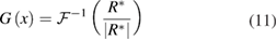
The moment of correlation plane approach (Bhattacharya et al 2018) relies on the hypothesis that the cross-correlation function is the convolution between the probability density function (pdf) of the particle image displacements and the average particle image intensity. Hence, the pdf of the particle image displacements in the interrogation window is calculated from the generalized cross correlation plane (GCC), computed as
where  is the inverse Fourier transform operator, R* denotes the Fourier transform of the cross-correlation plane, and |R*| is its magnitude, representing the average particle image contribution. The primary peak region of G(x) is the pdf of all possible particle image matches in the correlated image pair that contribute to the evaluation of the cross-correlation primary peak (figure 10). The standard uncertainty of the measured displacement is then evaluated from the second order moment of G(x) about the primary peak location. It should be noted that, due to the limited resolution in resolving the sharp GCC peak, Bhattacharya et al recommend convolving the GCC peak with a known Gaussian, whose diameter is estimated from the width of the primary peak of the cross-correlation plane. Such process introduces errors in the uncertainty estimate of the order of 0.02 pixels.

Figure 10. Schematic representation of how the displacement pdf is extracted from the from the cross-correlation of the PIV image pair. Figure reproduced from Bhattacharya et al 2018. © IOP Publishing Ltd. All rights reserved.
Download figure:
Standard image High-resolution image3.2.2.4. Error sampling method.
Closely related to the concept of nth-order replication introduced by Moffat (1982, 1985, 1988), the error sampling method (ESM, Smith and Oberkampf 2014) aims at estimating the uncertainty associated with unknown systematic error sources that affect a measurement. The main idea is to repeat the experiment several times after varying as many aspects as possible, including experimental facility and equipment. Variations in the measured quantities are representative of systematic errors due to either process unsteadiness or inaccuracies of the experimental apparatus. It should be remarked that, contrary to the other approaches discussed in this section, the error sampling method typically provides only the systematic uncertainty of statistical quantities, and not the random uncertainty of instantaneous velocity vectors.
Smith and Oberkampf (2014) employed the error sampling method to quantify the systematic uncertainty of the time-averaged velocity profile in a transient mixed-convection facility. Using the same equipment and facility, planar PIV measurements were repeated daily over the course of a month. The results showed that both wake position and peak velocity varied daily (figure 11). Furthermore and most important, the velocity variations were much larger than what could be predicted with standard uncertainty quantification and uncertainty propagation methods.
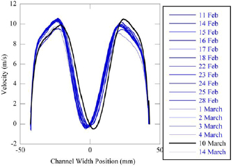
Figure 11. Time-average streamwise velocity profile measured in the transient mixed-convection facility over the course of a month. Figure reproduced from Smith and Oberkampf (2014). Copyright © 2014 by ASME.
Download figure:
Standard image High-resolution imageSimilarly, Beresh (2008) investigated the interaction between a supersonic axisymmetric jet and a transonic crossflow using three different experimental configurations, namely a two-component PIV setup and two stereoscopic PIV arrangements both in the streamwise plane and in the cross-plane. Furthermore, the raw data was processed with two different software packages. The results highlighted that stereoscopic data in the cross-plane yielded lower magnitude in the time-averaged velocity as well as in the turbulent stresses, and that lower discrepancies between streamwise and cross-plane measurements were achieved when using the processing algorithm that employs image deformation (Scarano and Riethmuller 2000).
Additional examples of error sampling methods for PIV include the use of multi-Δt image acquisition for estimation and correction of peak-locking and CCD readout errors (Nogueira et al 2009, 2011, Legrand et al 2012, 2018), processing PIV images with different calibration functions to quantify the calibration uncertainty (Beresh et al 2016), or comparing velocity fields from dual-frame image analysis algorithms with the more accurate ones retrieved with advanced multi-frame approaches for time-resolved PIV (Sciacchitano et al 2013).
4. Assessment and applications of a-posteriori UQ approaches
4.1. Assessment methods
To assess the performances of a-posteriori uncertainty quantification methods, the actual error must be known. However, the latter is inaccessible with standard PIV, which only returns the measured velocity field. Hence, several approaches have been proposed that provide the actual error or an accurate estimate of that. The standard approach consists of using synthetic images and Monte Carlo simulations, as already discussed in section 3.1.2 for the a-priori uncertainty quantification. In this case, the estimated uncertainty is compared with the known actual error (Timmins et al 2012, Sciacchitano et al 2013, Wieneke 2015), following procedures that will be discussed further in this section.
As synthetic images typically yield low measurement errors not fully representative of those encountered in real experiments (Stanislas et al 2005), methodologies have been devised which quantify with high degree of precision and accuracy the actual error in real experimental images. Those methodologies rely upon using additional information to determine the actual velocity field, stemming, for example, from theoretical knowledge or the usage of a more accurate measurement system. For instance, Charonko and Vlachos (2013) examined the laminar stagnation point flow around a rectangular body, for which the actual flow is known from the exact solution of the Navier–Stokes equations. Sciacchitano and Wieneke (2016) made use of a random pattern of dots mounted on a high-precision rotation stage. Knowing the magnification factor and the actual rotation of the stage, the measurement error could be readily retrieved.
When the actual velocity field is not known from theory or from a prescribed motion of the tracer particles, a dual-experiment can be conducted. An auxiliary measurement system is employed, typically indicated as high-dynamic-range (HDR, Neal et al 2015) or high-resolution (Boomsma et al 2016), to provide a velocity field that is more accurate than that retrieved with the standard measurement system (MS, also indicated as low-resolution LR). The high-resolution system can be a different measurement system (e.g. hot wire anemometer, laser Doppler velocimetry system), or an additional PIV system with higher image magnification. In the latter case, the underlying principle is that a larger displacement is measured in the image plane, resulting in a lower relative uncertainty with respect to the measurement system (Sciacchitano 2014). Timmins et al (2012) and Wilson and Smith (2013a) conducted separate data acquisitions with PIV and hot wire anemometry (HWA). The comparison between PIV and HWA data enabled determining the PIV systematic errors on the flow statistics (time-averaged velocity and Reynolds normal stress). However, since the measurements were carried out at different time instants, no information on the instantaneous error value could be retrieved. Neal et al (2015) carried out velocity measurements using three different systems simultaneously, namely a low-resolution two-component measurement system (MS, whose uncertainty was quantified with different a posteriori UQ methods), an HDR stereoscopic PIV system featuring optimal imaging conditions and four times higher image magnification, and a hot-wire anemometry system (single wire and cross-wire probes). To avoid interference between the PIV and HWA signals, the HWA probe had to be shielded from the laser light and was positioned about 2 mm downstream of the PIV field of view (figure 12(left)).
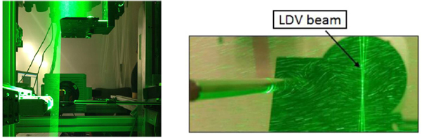
Figure 12. Example of dual-experiments for determination of the actual local and instantaneous velocity. Left: PIV and hot-wire anemometry (Neal et al 2015); © IOP Publishing Ltd. All rights reserved. Right: PIV and laser Doppler velocimetry (Boomsma et al 2016); © IOP Publishing Ltd. All rights reserved.
Download figure:
Standard image High-resolution imageSimilar to Neal et al (2015), Boomsma et al (2016) carried out simultaneous measurements with two PIV systems at different spatial resolution and a laser doppler velocimetry (LDV) system. Compared with the HWA system, the LDV system offers the advantage of being non-invasive and allowing velocity measurements at any point of the PIV field of view. However, the LDV signal cannot be synchronized with the PIV acquisition, as the LDV time series are not regularly sampled in time due to the random arrival time of the tracer particles. Additionally, the LDV laser beam is typically visible in the PIV images (figure 12(right)) and must be filtered out to avoid a local reduction of the image quality and in turn of the PIV measurement accuracy.
It is important to remark that, when designing and conducting dual-experiments, it is of paramount importance to achieve high correspondence between the measurement locations of reference and MS data. In fact, a small relative misalignment affects the comparison between MS and reference data, yielding over-estimated measurement errors. Typically, the calibration target alone is not sufficient for aligning the data sets and further alignment is necessary, which can be conducted by cross-correlating the velocity fields of the two systems, and determining whether a residual misalignment is present. Furthermore, it should be reminded that the velocity difference between MS and HDR provides not the actual MS error, but an estimate of that which is affected by the error of the HDR system. For this reason, the error magnitude of the HDR system should not exceed one fourth of the MS error (Sciacchitano et al 2015, Boomsma et al 2016).
Once the local and instantaneous measurement errors have been determined, a comparison with the quantified uncertainties can be conducted. A possible way of comparing the two quantities relies on the uncertainty coverage (or uncertainty effectiveness; Timmins et al 2012, Sciacchitano et al 2015), which describes the percentage of samples for which the measurement error lies within the uncertainty bands. To determine the uncertainty coverage, the expanded uncertainty must be determined at a selected confidence level. Notice that, while some of the PIV-UQ methods are able to compute the expanded uncertainty at any desired confidence level, others quantify only the standard uncertainty. In the latter cases, the expanded uncertainty must be computed based on hypotheses on the error distribution, typically assumed to be normal. Confidence levels of 68% or 95% (1-sigma and 2-sigma for normal error distribution, respectively) are usually considered for this analysis, with the former providing the more robust estimates in case of less well-converged statistics (Sciacchitano et al 2015). The closer the estimated uncertainty coverage to the selected confidence level, the more accurate the quantified uncertainty.
Alternatively, in absence of systematic errors (null mean error), the root-mean-square (RMS) of measurement error and standard uncertainty can be compared directly (Sciacchitano et al 2015). Such comparison does not require any assumption on the shape of the error distribution. However, it is assumed that the error and uncertainty data are statistical converged (large number of samples). The approach can be used even when the errors stem not from a single parent distribution, but from the superposition of several different ones with different variances. An extension of this concept consists of comparing the root-mean-square of the expanded uncertainty at C% confidence level with the C% percentile of the error magnitude (Xue et al 2014, Boomsma et al 2016).
4.2. Performance assessment studies
Several studies have been conducted to evaluate the accuracy of the a-posteriori uncertainty quantification approaches. Timmins et al (2012) assessed the performances of the uncertainty surface method based on synthetic images as well as on the comparison between PIV and HWA measurements. The numerical assessment relied on the uncertainty coverage computed at 95% confidence level. By finding that in many cases the estimated uncertainty coverage was significantly lower than 95%, the authors concluded that either an error source parameter (e.g. shear rate) had been estimated incorrectly, or an important error source (e.g. out-of-plane displacement, image noise) had been neglected. To enhance the coverage of their method, the authors proposed to introduce an 'uncertainty floor', or minimum possible value of uncertainty estimate, equal to 0.050 pixels for standard cross-correlation (SCC, Scarano and Riethmuller 2000) and 0.023 pixels for robust phase correlation (RPC, Eckstein and Vlachos 2009) image analysis. In the experimental assessment, larger discrepancies between HWA and PIV data were retrieved at the lower particle image displacements, which also corresponded to larger uncertainty values estimated with the uncertainty surface method.
Similarly, Charonko and Vlachos (2013) assessed the performances of the PPR method based on both synthetic and experimental images, conducting an uncertainty coverage analysis both at 68% and 95% confidence level. The reliability of the PPR method was found to be higher for the RPC analysis than for the SCC analysis, which was attributed to the wider range of cross-correlation primary peak ratio values in the former image evaluation algorithm. Based on the same numerical and experimental test cases as in Charonko and Vlachos (2013), Xue et al (2014, 2015) assessed the performances of the PPR, PRMSR, PCE, cross-correlation entropy and MI methods. The authors concluded that the differences between theoretical coverages and calculated values were below 5% for all metrics.
By comparing the root-mean-square of the actual error with that of the estimated uncertainty, Sciacchitano et al (2013) showed the sensitivity of the particle disparity method to the most common error sources in PIV measurements. Furthermore, the authors report that the uncertainty of real experiments was quantified with accuracy exceeding 60% (discrepancy between uncertainty and actual error root-mean-square below 40%); lower accuracy was retrieved in presence of peak locking errors. Wieneke (2015) assessed the correlation statistics method via synthetic images considering similar parameters as in the analysis of Sciacchitano et al (2013). The method showed good agreement between estimated uncertainty and actual error RMS for varying random Gaussian noise, particle image size and density, in-plane and out-of-plane displacement.
Bhattacharya et al (2018) assessed the performances of the moment of correlation method based on both synthetic and experimental test cases. The authors found that the RMS of the predicted uncertainty followed the trend of the error RMS for a wide range of variation of typical PIV error sources. The agreement between the two quantities was good especially for processing with large window sizes, whereas for the smaller window sizes a bias of the order of 0.02 pixels was noticed, which caused overestimated uncertainty values.
Some recent works focused on the comparative assessment of the performances of different a-posteriori uncertainty quantification approaches. Sciacchitano et al (2015) compared the uncertainty surface (US), particle disparity (PD), peak ratio (PR) and correlation statistics (CS) methods based on the measurements of a rectangular transitional jet flow (figure 13). The image recordings were analyzed with the LaVision DaVis 8.1.6 software.
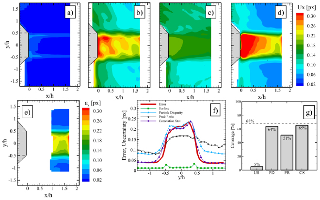
Figure 13. Comparison between root-mean-square uncertainty and error in the jet flow experiment in presence of out-of-plane motion in the jet core. Top row: Root-mean-square of the estimated uncertainty. (a) Surface method; (b) particle disparity method; (c) peak ratio method; (d) correlation statistics method. Bottom row: (e) Error root-mean-square; (f) comparison between error and uncertainty RMS along a profile at x/h = 1.5. Statistical results computed over time; (g) uncertainty coverage at 68% confidence level in the jet core, where the out-of-plane particle displacement is the highest. Figure readapted from Sciacchitano et al (2015). © IOP Publishing Ltd. All rights reserved.
Download figure:
Standard image High-resolution imageThe comparative assessment showed that, among the four methods, the correlation statistics approach provided the most reliable uncertainty estimates, with accuracy over 85% for most cases, and of the order of 75% even in presence of peak locking and low seeding concentration. Furthermore, the method showed good sensitivity to error variations in the range between 0.03 and 0.25 pixels. Boomsma et al (2016) extended the comparative assessment of methods to different image analysis software, namely PRANA from Purdue University, Insight 4G from TSI and DaVis from LaVision GmbH. The authors compared the performances of the primary peak ratio (PPR), mutual information (MI), image matching (IM, same as particle disparity) and correlation statistics (CS) uncertainty quantification approaches. The assessment was based on experimental data of a jet flow and a flow over a cylinder, where the reference velocity was provided by a high-resolution PIV system. With respect to the work of Sciacchitano et al (2015), the PPR method showed significantly improved performance (see figure 14), which was attributed both to the improved calibration model of Xue et al (2014), and to the use of the robust-phase correlation image analysis (Eckstein and Vlachos 2009).
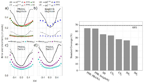
Figure 14. Left: RMS error and uncertainty profiles along the spanwise direction across the jet flow for the following PIV-UQ methods (and image analysis algorithm): (a) PPR (PRANA); (b) PPR (Insight4G); (c) and (d) IM (PRANA) and CS (DaVis) for X and Y displacement components, respectively. UB represents the upper uncertainty bound (84.25% of the error magnitude distribution), LB the lower uncertainty bound (14.75% of the error magnitude distribution). Right: Standard coverage for the jet flow experiment at 68.5% confidence level. Figure reproduced from Boomsma et al (2016). © IOP Publishing Ltd. All rights reserved.
Download figure:
Standard image High-resolution image4.3. Survey of applications
Applications of a-posteriori UQ methodologies have been reported for a wide range of fluid mechanics problems, especially those involving the measurement of unsteady turbulent flows. Quinn et al (2014) and Floryan et al (2017) made use of the particle disparity method to characterize the uncertainty of the unsteady wake of a pitching wing in the incompressible flow regime, retrieving uncertainty values of the order of 1% to 5% of the free-stream velocity. Similar results are reported by Pascioni and Cattafesta (2018), who employed the correlation statistics method to determine the uncertainty of the unsteady slat-cove flow field at Re = 1.7 × 10⁶. Using the particle disparity method, Shan et al (2014) characterized the uncertainty behind a circular orifice in a round pipe flow at Re = 25 000; the authors report that the highest uncertainty of the order of 0.15–0.30 pixels is found in the near-wall and the shear-layer regions.
Applications of different a-posteriori PIV-UQ methodologies for measurements of vortical and swirling flows are reported among others by Yang et al (2016), Lignarolo et al (2016), Rajamanickam and Basu (2017) and Marimon Givannetti et al (2017), highlighting that flow measurements in the vortex core feature uncertainty values up to one order of magnitude larger than those in the outer regions (figure 15(top-left)). Further applications aimed at the characterization of the instantaneous velocity uncertainty in jet flows (Pieris 2017, Charonko and Prestridge 2017), turbulent flows (Dou et al 2016, Elhimer et al 2017), natural convection (Naghib et al 2017), flow control investigations (Yarusevich and Kotsonis 2017, Singh et al 2018), aeroacoustics investigations (Arce León et al 2016, Nickels et al 2016, Upadhyay et al 2017), turbomachinery problems (Saini et al 2016), combustion problems (Andreini et al 2016, Ebi and Clemens 2016), characterization of test facilities (Chikishev et al 2016) and building aerodynamics (Sánchez et al 2017). Despite most applications deal with subsonic flows, several works made use of a-posteriori PIV-UQ approaches in the transonic (Scharnowski et al 2017, Beresh et al 2017a), supersonic (Davis and Kumar 2015, Kreth et al 2016, Valentich et al 2016, Beresh et al 2017b, Mohaghar et al 2017) and even hypersonic (Zhu et al 2018) flow regimes. However, it should be remarked that the a-posteriori UQ methods presented in section 3.2 are unable to quantify the uncertainty associated with the particle slip, which may be predominant especially in hypersonic flows.
Figure 15. Examples of applications of a-posteriori PIV-UQ methods. Top-left: Mean uncertainty of the w-velocity component (expressed in pixel units) for a wing tip vortex flow. Uncertainty quantified with the correlation statistics method. Figure reproduced from Marimon Giovannetti et al (2017). Copyright (2017) with permission from Elsevier. Top-right: Velocity uncertainty in m/s estimated with the primary peak ratio method in a coronary bifurcation model (internal nominal diameter: 3.96 mm; inlet velocity: 0.2 m s−1). Figure reproduced from Raben et al (2015). © 2014 Società Italiana Biomateriali. Bottom-left: Time-averaged velocity uncertainty field for a 1 mm diameter supersonic free jet at Mach 1.80. Uncertainty quantified with the correlation statistics method. Figure reproduced from Kreth et al (2016). © Springer-Verlag Berlin Heidelberg 2016. With permission of Springer. Bottom-right: Time-averaged velocity uncertainty field for a 25.4 mm diameter supersonic free jet at Mach 1.5. Uncertainty quantified with the uncertainty surface method and expressed as percentage of the jet velocity. Figure reproduced from Davis and Kumar (2015). © Springer-Verlag Berlin Heidelberg 2014. With permission of Springer.
Download figure:
Standard image High-resolution imageAside from physical discovery experiments, a-posteriori UQ methodologies have been employed for validation benchmark experiments, aimed at providing a database for the validation of CFD simulations. Examples of such applications include combustor flows (Andreini et al 2017), forced convection flows (Harris et al 2016) and biomedical flows (Raben et al 2015, Paliwal et al 2017).
Additionally, a-posteriori UQ approaches have been used to enhance the quality of the experimental results, either by supporting the selection of experimental parameters (Persoons 2015), or by providing an input for the suppression of noisy fluctuations via data post-processing or data assimilation approaches (de Baar et al 2014, Brindise and Vlachos 2017, Wieneke 2017a, Symon et al 2017).
As a final remark, the successful applications of a-posteriori UQ approaches in very diverse fluid mechanics problems and for different purposes confirm that the PIV uncertainty varies largely in space and time, and from experiment to experiment (see figure 15). Variations by factor three among different velocity components and by one order of magnitude among different locations of the flow field have been reported. Such uncertainties can be significantly larger or smaller than the universal uncertainty constant of 0.1 pixels or than values obtained based on synthetic data and Monte Carlo simulations, and therefore require accurate evaluation via a suitable a-posteriori UQ approach.
5. PIV uncertainty propagation
The aim of PIV measurements is seldom limited to the determination of instantaneous velocity fields, but often extends to the evaluation of derived statistical (e.g. time-averaged velocity, Reynolds stresses, higher order statistical moments) or instantaneous quantities (e.g. vorticity, acceleration). Additionally, instantaneous and time-averaged pressure fields can be retrieved from the measured velocity fields (van Oudheusden 2013). Hence, once the instantaneous velocity fields have been computed and the uncertainty of those quantified, uncertainty propagation approaches are employed to quantify the uncertainty of the derived quantities of interest.
As in many other fields of experimental science and engineering, uncertainty propagation for PIV data is typically conducted via the Taylor series method (TSM) or the Monte Carlo method (MCM). Consider a quantity of interest r, function of N measured variables:

In the TSM, the combined standard uncertainty of r, accounting for both systematic and random uncertainties (b and s, respectively) of the measured variables, is computed as (Coleman and Steele 2009):

where  are the sensitivity coefficients and bij and sij represent the correlated systematic and random uncertainties, respectively.
In the MCM, for each error source, a random sample is taken from its distribution and added to the measured variable xi; the resulting quantity of interest r is then computed. The process is repeated until a converged distribution of r is determined, from which the uncertainty of the latter is evaluated.
Detailed discussions about the theory of these approaches and their implementation is reported in standard textbooks (e.g. Bendat and Piersol 2010, Coleman and Steele 2009) and papers (George et al 1978, Benedict and Gould 1996). In the following, the discussion will focus on the peculiarities of applying these methods for uncertainty propagation in PIV.
5.1. Uncertainty of derived statistical properties
Several studies have focused on the propagation of the uncertainty from the instantaneous velocity components to the statistical quantities of interest. Gui et al (2001a) conducted a thorough uncertainty analysis based on the Taylor series method to quantify the uncertainty of mean velocity, velocity variance and covariance (Reynolds normal and shear stresses, respectively) in the wake of a model-scale ship. The authors made use of the uncertainty propagation formula (13) considering the contributions to the total uncertainty of object size, image size (and therefore scaling factor), laser-pulse separation time, measured particle-image displacement, free-stream velocity measurements and coordinate deviations. Both systematic uncertainty and precision uncertainty were accounted for. The systematic uncertainties were estimated from calibration (object size, image size and coordinates deviation), listed from manufacturer's specifications (laser-pulse separation time), taken from previous estimates (free-stream velocity) or computed with experiments and simulations (measured particle image displacement). Adeyinka and Naterr (2005) used an approach analogous to that of Gui et al (2001a) to determine the uncertainty of the local entropy production evaluated from PIV and LIF measurements. Wilson and Smith (2013a) extended the work of Gui et al (2001a) by removing the simplifying assumption that the mean bias is only function of one error source, the true velocity. In contrast, they estimated the instantaneous bias and random uncertainty via the uncertainty surface method of Timmins et al (2012). Furthermore, they distinguished between perfectly correlated biases (bij = bi bj ) and uncorrelated biases (bij = 0). The authors pointed out that bias errors are often correlated in PIV experiments, where instantaneous quantities are affected by identical calibrations, system biases (e.g. temperature effects) and algorithm processing. For the case of correlated biases, the expression of the uncertainty of the mean reads
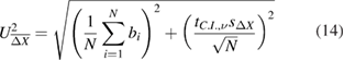
where sΔX is standard deviation of the samples, N the number of (statistically independent) samples, and tC.I.,ν is the t-statistic describing the desired confidence interval, with ν = N − 1 degrees of freedom (Bendat and Piersol 2010). The first term on the right-hand-side represents the bias uncertainty, whereas the second term is the random (precision) uncertainty due to the finite ensemble size. It should be remarked that bias uncertainty estimates are typically very difficult to obtain (to date, only Timmins et al's (2012) uncertainty surface method provides direct access to the bias uncertainty). To quantify the systematic uncertainty associated with the spatial modulation due to the finite interrogation window size, it is recommended to process the PIV images with different interrogation window sizes and report the variability of the results. Additionally, it should be noted that the determination of the uncertainty of the mean does not require the knowledge of the random uncertainty of the instantaneous measurements (which is included in sΔX).
While a symmetric uncertainty (upper bound equal to the lower bound) was computed for the mean, an asymmetric uncertainty was estimated for both variance and covariance. In particular, the lower bound was proven to be larger than the upper bound, as the variances of random and systematic errors always lead to overestimate the true measured variance and covariance. Wilson and Smith (2013b) assessed the accuracy of the estimated uncertainty of the mean velocity and the Reynolds normal stresses via comparison between PIV and HWA measurements in a jet flow. The uncertainty propagation methodology was demonstrated considering variations of tracer particles concentration, velocity gradient, particle image size and displacement. The image analysis was conducted with two different algorithms, namely LaVision DaVis 7.2 and PRANA from Purdue University. As shown in figure 16, the uncertainty was typically underestimated when using the DaVis algorithm, whereas it exhibited relatively higher coverage when using the PRANA algorithm.
Figure 16. Left: Profile of the time-averaged velocity magnitude from hot-wire and PIV measurements (DaVis 7.2 and PRANA) with 0.5 pixels displacement in the jet core. Right: Reynolds normal stress for varying particle image displacement. Figure readapted from Wilson and Smith (2013b). © IOP Publishing Ltd. All rights reserved.
Download figure:
Standard image High-resolution imageIn Sciacchitano and Wieneke (2016), the expression of the uncertainty of several statistical quantities was derived by following an approach analogous to that of Wilson and Smith (2013a). Contrary to the latter authors, Sciacchitano and Wieneke focused on random errors and uncertainties, assuming that each systematic error of known sign and magnitude had been removed. As proposed by Brown et al (1996), the correlation terms in equation (13) were computed as

ρ (δxi, δxj ) being the cross-correlation coefficient between the errors of xi and xj , with –1 ⩽ ρ (δxi, δxj ) ⩽ 1. The authors pointed out that the errors of measurements adjacent in space or time may feature some degree of correlation, so in general ρ (δxi, δxj ) ≠ 0. As most PIV-UQ methods are unable to compute the value of ρ (δxi, δxj ), it is advised to determine the latter beforehand by synthetic images and Monte Carlo simulations. Furthermore, the authors highlighted the relevance of using the effective number of uncorrelated samples Neff for the evaluation of the precision uncertainty in equation (14). Neff may significantly differ from the total number of samples N (typically Neff ⩽ N) especially for time-resolved measurements conducted with high-speed PIV systems, where the relatively high acquisition frequency causes non-null temporal correlation among the samples (Thiébaux and Zwiers 1984, Falchi and Romano 2009). A detailed discussion on the evaluation of Neff and its implications on the uncertainty of the mean of correlated data is reported in Smith et al (2018). Charonko and Prestridge (2016) made use of the Taylor series method to evaluate the uncertainty of the turbulence dissipation rate, accounting for both random errors in the measured velocity field and systematic errors due to PIV image evaluation and spatial differentiation.
Resampling algorithms such as jackknife (Tukey 1958) and bootstrap (Efron 1979) are alternative approaches to determine the uncertainty of turbulence statistics. These approaches estimate the precision uncertainty of the sample statistics by using subsets of the available data. Each subset is employed to compute the desired sample statistics, and the results from different subsets yield a distribution of the latter, from which its uncertainty is evaluated. The main advantage of these methods is their general applicability in case of unknown error distribution, or unknown formula for the calculation of the standard uncertainty. For this reason, they are suitable for the evaluation of the uncertainty of higher order turbulence statistics (Benedict and Gould 1996). Stafford et al (2012) conducted low-speed PIV measurements to examine the turbulent flow at the outlet of a radial fan. The authors focused on the convergence of first (mean and turbulence intensity x- and y-velocity components) and second order statistics (Reynolds shear stress) by analysing the precision uncertainty as a function of the sample size N. By comparing the uncertainty estimated from Taylor series method formulae with that computed via bootstrap, the authors concluded that both approaches yielded comparable results for N > 103. The bootstrap approach showed the added value of providing the error distribution of the measured statistics, without requiring any assumption. Theunissen et al (2008) proposed the dependent circular block bootstrapping approach to account for the samples temporal correlation, which plays an important role when time-resolved PIV measurements are conducted. The authors demonstrated the approach for the determination of the confidence intervals of the sample mean, considering both cases of uncorrelated samples and highly correlated samples. Chatellier et al (2013) discussed the use of multi-block acquisition to quantify the uncertainty of sample statistics. The principle is to acquire blocks of correlated samples from time-resolved PIV measurements, each block separated by a relatively large time interval to ensure that the blocks are uncorrelated among each other. Based on laser-Doppler velocimetry data, the authors showed the superiority of this technique with respect to standard bootstrap, where the temporal correlation among samples is not accounted for.
5.2. Uncertainty of derived instantaneous properties
PIV measurements are often carried out to detect vortices and quantitatively evaluate their instantaneous parameters, such as location, extension and some measure of strength (Vollmers 2001). Instantaneous kinematic variables such as vorticity, circulation, shear rate and strain rate are directly computed from the measured velocity field by means of spatial differentiation. To quantify the uncertainty of such instantaneous quantities, Monte Carlo method or Taylor series method are usually employed. Using synthetic images simulating an Oseen vortex flow, Luff et al (1999) investigated how the measurement errors propagate from the velocity field to the vorticity field. The authors considered different algorithms for the computation of the latter, as well as different spatial filters for both the velocity and vorticity fields. From their analysis, Luff et al concluded that the lowest vorticity uncertainty is obtained using the standard three-point finite difference vorticity algorithm, and by filtering the velocity data with local polynomial regression and Gaussian smoothing. Similarly, Fouras and Soria (1998) derived theoretical expressions for the transmission of the random velocity errors into random vorticity error, and showed that the effect of random velocity errors is to increase the vorticity scatter. Furthermore, increasing velocity spatial sampling separation introduces a larger bias error, resulting in underestimation of the peak vorticity. More recently, Ma and Jiang (2018) showed that perspective errors in 2D2C PIV induce systematic errors in the measured vorticity, which are proportional to the in-plane derivatives of the out-of-plane velocity component.
Based on Taylor series method, Sciacchitano and Wieneke (2016) derived the expression of the standard uncertainty of the vorticity evaluated by central-difference scheme:
In equation (16) U is the local standard uncertainty of the velocity (assumed to be equal for both velocity components), h is the grid spacing (assumed to be uniform in both x- and y -directions) and ρ (2h) is the cross-correlation coefficient of the measurement error at two grid points at spatial separation 2h. The equation was obtained accounting for only random errors, and neglecting any systematic errors due to truncation and spatial modulation. An analogous expression was obtained for the 2D divergence of the velocity. In general, the spatial correlation of the measurement error (0 < ρ (2h) ⩽ 1) yields reduced vorticity uncertainty with respect to the case of uncorrelated velocity errors (ρ (2h) = 0). The value of ρ (2h) for a specific processing algorithm can be evaluated via synthetic images and Monte Carlo simulations; Sciacchitano and Wieneke report ρ (2h) = 0.45 for 32 × 32 pixels interrogation window and 75% overlap factor, whereas ρ (2h) becomes null for overlap factors of 50% or lower.
5.3. Stereo-PIV uncertainty quantification
Uncertainty analysis for stereoscopic PIV has been mainly conducted a priori via propagation of the uncertainty of the displacement measured by the two cameras and of the geometrical parameters (namely optical magnification, cameras angle and distances, object distance). The analysis has been carried out both for translation stereoscopic systems (Arroyo and Greated 1991, Prasad and Adrian 1993, Lawson and Wu 1997, among others) as well as for angular displacement systems (Lawson and Wu 1997, Zang and Prasad 1997, among others). Assuming uncorrelated variables and perfect registration, Prasad (2000) demonstrated that the random uncertainty of the out-of-plane velocity component is tan(θ) times larger than that of the in-plane velocity components, being θ the semi-angle between the two cameras. Furthermore, the random uncertainty of the in-plane velocity components is  smaller than that from a single camera, as both cameras contribute equally to the final result. Additionally, perspective errors are removed by the stereoscopic arrangement, whereas they can be significant in single-camera PIV measurements. Willert (1997) compared the stereo-PIV random uncertainty predicted from linear error propagation with that directly evaluated via measurements in a quiescent flow. The predicted uncertainty of the in-plane velocity component matched the measured value, whereas the uncertainty of the out-of-plane velocity component exceeded by about 10% the predicted value. Van Doorne et al (2003) extended the uncertainty analysis for the case of finite registration (systematic) errors, which may arise due to inaccurate mapping function from the image plane to the physical plane, or because of a misalignment between the centre of the light sheet and the location of the calibration grid (Coudert and Schon 2001). The latter are typically corrected for by using a self-calibration procedure (Wieneke 2005). Nevertheless, large stereoscopic angles and thick laser sheets can introduce substantial bias errors in the velocity even after a converged self-calibration, especially in presence of small particle image diameters and high seeding density or out-of-plane velocity gradients (Beresh et al 2016).
Only recently, Bhattacharya et al (2016) have introduced a framework to quantify a posteriori the uncertainty in each step of the stereo-PIV measurement chain, and to propagate the elemental uncertainties into the reconstructed velocity components. The framework, summarized in the flow chart of figure 17, accounts for the uncertainty of the physical coordinate positions, the triangulated z-plane location and the mapping function coefficients to determine the uncertainty of the stereoscopic angles. Finally, the latter is combined with the uncertainty of the planar velocities measured by the two cameras to compute the uncertainty of the three velocity components. The authors found that, after application of the self-calibration procedure, the uncertainties of the stereoscopic velocity components were dominated by the uncertainties of the planar velocity estimates. The uncertainty coverage of the proposed framework exhibited good agreement with the theoretical values in both Monte Carlo simulations and experimental assessment.

Figure 17. Uncertainty propagation flow chart for stereoscopic PIV. (a)–(c) uncertainty of physical coordinate systems; (d) and (e): uncertainty of the triangulated z-location; (f) and (g) uncertainty of the mapping function coefficients; (h) uncertainty of the stereoscopic angles; (i) uncertainty of the planar velocity measurements; (j) combined uncertainty of the stereoscopic PIV measurement. Figure reproduced from Bhattacharya et al (2016). © IOP Publishing Ltd. All rights reserved.
Download figure:
Standard image High-resolution imageDespite its recent publication, Bhattacharya et al's framework for stereo-PIV uncertainty quantification has been successfully employed already for several flow measurements both in the subsonic and supersonic flow regimes, for applications on synthetic jets (Paolillo et al 2017), biomedical flows (Medero et al 2018), internal flows in nuclear reactor models (Nguyen and Hassan 2017, Nguyen et al 2018), supersonic jets (Beresh et al 2017a, Beresh 2018) and shock-wave boundary-layer interaction (Vanstone et al 2018). The framework's application to experimental data showed that the typical stereo-PIV uncertainty is in the range 0.07–0.4 pixels, and that the out-of-plane displacement component suffers of 2 to 3 times larger uncertainty than the in-plane displacement components.
5.4. Volumetric PIV/LPT uncertainty quantification
In volumetric flow measurements by tomographic PIV (Elsinga et al 2006b, Scarano 2013) or 3D Lagrangian particle tracking (LPT, Maas et al 1993), the quantification of the measurement uncertainty is further complicated by the use of multiple cameras from different viewing angles and the reconstruction of the 3D distribution of the particle images. For example, the tomographic reconstruction contains spurious intensity peaks, referred to as 'ghost particles' (Elsinga et al 2006a), which have the effect of biasing the computed velocity gradients (Elsinga et al 2011, Elsinga and Tokgoz 2014). However, the issue of ghost particles is reduced considerably when making use of the temporal information contained in time-resolved acquisitions (Novara et al 2010, Lynch and Scarano 2015, Schanz et al 2016).
Due to the additional complexities above, the topic of uncertainty quantification for 3D-PIV/LPT is still considered in its infancy (Discetti and Coletti 2018), and has been mainly tackled via a priori approaches based on synthetic images and Monte Carlo simulations (see for instance cases C and D of the 4th International PIV challenge, Kähler et al 2016). A posteriori approaches based on the compliance with the conservation of mass for incompressible flows (solenoidal velocity field) have been applied to quantify the uncertainty of the measured velocity components and their spatial derivatives (Scarano and Poelma 2009, Atkinson et al 2011, Lynch and Scarano 2014). In case of time-resolved flow measurements of incompressible flows, the compliance with the vorticity transport equation has been proposed as an alternative to the velocity divergence approach (Novara 2013). Extension of the particle disparity approach to tomographic PIV was investigated by Sciacchitano and Lynch (2015) in the attempt to quantify the uncertainty of each velocity component, without relying on the hypothesis of flow incompressibility.
For Lagrangian particle tracking, an additional error source arises from the interpolation of the scattered velocity vectors onto a Cartesian grid. A method for the direct quantification of such uncertainty was proposed by Schneiders and Sciacchitano (2017), where a small percentage of the tracks is used as a benchmark to evaluate the accuracy of the velocity interpolation obtained from the remaining trajectories.
Future advances in uncertainty quantification for volumetric velocimetry measurements are envisaged to focus on Lagrangian particle tracking approaches, which have shown their superiority with respect to correlation-based image analysis (Kähler et al 2016). In the latter case, the main challenge is to quantify the uncertainty of the measured particles trajectories, discerning between correct and incorrect trajectories and between physical and spurious velocity fluctuations along each trajectory.
5.5. Uncertainty of pressure and pressure gradient
Determination of the static pressure from PIV velocity data has become common in the last decade (van Oudheusden 2013). The overall uncertainty of the retrieved static pressure field depends upon several parameters, which include (Charonko et al 2010, de Kat and van Oudheusden 2012, van Oudhesden 2013, Azijli et al 2016, Pan et al 2016, McClure and Yarusevych 2017): uncertainty of the underlying velocity field; measurement spatial and temporal resolution; approach employed to compute the material acceleration; uncertainty of the boundary conditions; pressure integration procedure; modelling errors when planar PIV data are used to reconstruct the pressure field in a 3D flow.
De Kat and van Oudheusden (2012) developed a framework based on Taylor series method for the propagation of the velocity uncertainty through the material acceleration, considering both Eulerian and Lagrangian formulation of the latter. In their analysis, the authors assumed the velocity errors uncorrelated in space and following a normal distribution, obtaining

where h is the grid spacing and Δt is the time separation between subsequent velocity fields. Notice that the assumption of velocity errors uncorrelated in space yields overestimated uncertainty values compared to the more realistic case where the spatial correlation of adjacent velocity vector is accounted for (Sciacchitano and Wieneke 2016). The overestimation is equal to  for the Eulerian formulation, whereas it is typically negligible for the Lagrangian formulation, which relies on the difference of velocity vectors at different time instants, whose errors can be assumed to be uncorrelated. De Kat and Ganapathisubramani (2012) and Laskari et al (2016) extended the analysis by considering the case of time-resolved volumetric PIV measurements, as well as non-time-resolved measurements where the application of Taylor's hypothesis is required for the determination of the pressure gradient. For the case of material acceleration evaluated from the Eulerian perspective (equation (17)), an analytical uncertainty model that includes also the truncation error terms arising from the finite resolution of the derivative estimators was developed by McClure and Yarusevych (2017a). Van Gent et al (2018) further expanded the theoretical framework to consider the case where the material acceleration is computed not by simple central differencing between two points, but via pseudo-tracking of a fluid parcel with multiple integration steps. In the latter case, positional errors incurred at a previous integration steps yield additional (often correlated) position and velocity errors in subsequent integration steps. Furthermore, the authors developed an analytical expression for the uncertainty in the case where the material derivative is computed via least-square regression of the velocity values along the pseudo-track, showing that the latter approach is more effective in suppressing the velocity errors. Finally, an upper bound for the uncertainty associated with numerical interpolation and integration procedures was determined. Pan et al (2016) set up a theoretical framework for the quantification of the uncertainty of the static pressure field evaluated via solution of the Poisson equation. The authors analytically quantified the uncertainty bound of the pressure field investigating how the measurement errors propagate through the Poisson equation. The effects of size of the flow domain, flow type, shape, type and uncertainty of the boundary conditions were thoroughly scrutinized, proving that the boundary conditions type has a major influence on the pressure uncertainty, especially for small-sized flow domains.
An approach to reconstruct the instantaneous pressure gradient error was proposed by McClure and Yarusevych (2017b), based on the solution of a divergence-curl system. Assuming error-free boundary conditions, the authors showed that an approximate field for the pressure gradient error could be reconstructed. Subtraction of the error field from the measured pressure gradient yielded more accurate pressure estimates across the inner domain (figure 18(top)). A Bayesian framework for the a-posteriori uncertainty quantification of PIV-based pressure data was introduced by Azijli et al (2016). In such framework, the posterior distribution (probability distribution of the true velocity, given the PIV velocity measurement) is retrieved from the prior distribution (prior knowledge of the velocity field, e.g. compliance with the constitutive equations of fluid motion), and the statistical model of the velocity uncertainty. The posterior is then propagated through the discretised Poisson equation for pressure, yielding the probability density function of the measured static pressure field. The work also provides an expression based on Taylor series method for the pressure uncertainty computed via solution of the Poisson equation, which relies on the simplifying assumption of spatially uncorrelated velocity errors. Comparison between the two a-posteriori UQ approaches highlighted the superiority of the Bayesian framework. The highest accuracy of the pressure uncertainty was retrieved when using a solenoidal prior and the Lagrangian formulation for the material acceleration, returning coverage values of 68% and 94% for the 1-σ and 2-σ uncertainty, respectively (figure 18(bottom)).
Figure 18. Top: Lamb-Oseen vortex pressure field. Comparison between solutions without (first row) and with (second row) correction for the pressure gradient errors. Figure reproduced from McClure and Yarusevych (2017b). © Springer-Verlag Berlin Heidelberg 2017. With permission of Springer. Bottom: Comparison between reference pressure time series from microphone measurements (red) and PIV (black) in a turbulent boundary layer. The gray regions represent the uncertainty estimated via the Bayesian framework at 68.3% confidence level. Figure reproduced from Azijli et al (2016). CC BY 4.0. © The author(s) 2016.
Download figure:
Standard image High-resolution image
6. Conclusions
Uncertainty quantification of PIV data has become a topic of great interest within the PIV community. In the early days, PIV-UQ was mainly tackled a priori, aiming to determine a general figure for the accuracy of the PIV technique. This was done either by theoretical modelling of the measurement chain, or via synthetic images and Monte Carlo simulations, or by dedicated experiments with a known particle motion. More recently, the attention has shifted towards the data-based a-posteriori uncertainty quantification, which proposes to quantify the local and instantaneous uncertainties of the measured velocity fields. Indirect and direct methods have been introduced. The former make use of pre-calculated information typically obtained by calibration, whereas the latter extract the measurement uncertainty directly from the image plane using the estimated displacement as prior information. Assessments of those a-posteriori UQ approaches have been conducted both numerically via Monte Carlo simulations and experimentally via dedicated experiments, where the actual flow velocity is known either from theory or from the use of more accurate measurement systems (dual-experiment). Comparative assessment studies have highlighted strengths and weaknesses of those approaches in different flow and imaging conditions. In particular, indirect methods typically provide more complete information on the measurement uncertainty (e.g. both systematic and random uncertainty, error distribution, capability to quantify the uncertainty associated with outliers), but have shown relatively lower sensitivity to variations of the measurement errors. Conversely, direct methods usually return no or limited information on the error distribution (the estimate of which, when available, is affected by truncation errors due to the finite number of particle images in an interrogation window), but more accurately predict the uncertainty in the range 0.03–0.3 pixel units. Successful applications of both direct and indirect a-posteriori UQ approaches have been reported in a wide range of applications and fluid mechanic problems from subsonic to hypersonic flows. However, the experimenter should keep in mind that these approaches only quantify the uncertainty that is encoded in the recorded images, whereas 'hidden' error sources due to, for example, non-uniform inflow, variations of Reynolds or Mach numbers during the experiment, particle slip, system calibration, timing and synchronization must be evaluated separately.
The propagation of the estimated uncertainty of the velocity to derived flow properties, either instantaneous (e.g. vorticity, pressure) or statistical (e.g. time-average or Reynolds stresses), has been tackled via the Taylor series and Monte Carlo methods. It can be concluded that nowadays the experimenter can count on suitable tools to conduct detailed uncertainty analyses in planar PIV measurements, and that the 'universal uncertainty constant' of 0.1 pixel units should be regarded only as a preliminary rough (and overly simplistic) estimate of the PIV uncertainty. For three-component measurements by stereoscopic PIV and volumetric measurements by tomographic PIV and LPT, the quantification of the measurement uncertainty is complicated by the use of multiple cameras. While the theoretical framework for the uncertainty quantification in stereo-PIV has been developed, uncertainty quantification of volumetric PIV/LPT data is a topic of ongoing research. Considering the recent advances in volumetric flow measurements, which rely more and more on Lagrangian particle tracking rather than on correlation-based analysis, it is envisaged that future advances in PIV-UQ will focus on determining the accuracy of the estimated particle tracks and on the uncertainty associated with unresolved length scales.
Finally, it should be remarked that while much effort has been conducted for the a-posteriori quantification of the random uncertainty, relatively less studies have attempted the a-posteriori quantification of the PIV systematic uncertainty. The latter, mainly ascribed to calibration errors, truncation errors in space or time (unresolved or under-resolved length or time scales) or peak locking, plays a chief role especially for the investigation of unsteady and turbulent flows. It is envisaged that novel protocols will be devised in the near future employing multiple acquisition (e.g. laser sheet thickness, optical aperture, pulse separation time as in Scharnowski et al (2019)) and processing parameters (e.g. interrogation window size and weighting) in the same experiment to enable the accurate quantification also of the systematic uncertainty.
Acknowledgments
Dr Bernhard Wieneke is kindly acknowledged for the many productive conversations about PIV-UQ and for his valuable comments on this manuscript. This work was conducted as part of the Veni project 15854 'Deploying Uncertainty Quantification in Particle Image Velocimetry', funded by the Dutch Research Organization NWO domain Applied and Engineering Science.
Footnotes
- 1
Alternative classifications exist. The ISO-GUM (2018) distinguishes type A and type B evaluations of the standard uncertainty. The former consists of performing data statistics on repeated observations, whereas the latter relies on previous measurement data, general knowledge of the behavior and properties of the instruments, manufacturer's specifications, calibration data or comparison with a more accurate measurement system. In the modelling and simulation communities, uncertainties are classified into aleatory (or stochastic), stemming from random events, and epistemic, due to lack of knowledge. Finally, the precision uncertainty is defined as the random uncertainty of a statistical quantity computed from a finite number of samples.