

Abstract
The geometric errors of numerical control (NC) rotary tables can be measured using a single instrument according to the conventional measurement method. This study presents an efficient method for this measurement using four-station laser tracers. A 3D coordinate measurement algorithm of the four-station laser tracer was established, the self-calibration of the laser tracer position and the spatial measuring point algorithm was realized, and the volumetric error of the measuring point on the rotary table was obtained. Then, the geometric errors of the NC rotary table were modeled using the screw theory, and a three-point measurement method was proposed to realize the separation of these geometric errors. Using the geometric error measurement experiment, six geometric errors of the NC rotary table were obtained. Compared with the conventional standard ball and laser interferometer measurement methods, the radial and axial runout results obtained using the laser tracer show differences of 0.08 and 0.07 µm, respectively, and the result of positioning error measurement shows a difference of 2.2 µrad. In addition, the method proposed in this study demonstrates an efficiency improved by five times, under the premise of ensuring the measurement accuracy, which broadens the possibilities for applications of rotation axes' geometric error measurement in machining centers.
Export citation and abstract BibTeX RIS

Original content from this work may be used under the terms of the Creative Commons Attribution 3.0 licence. Any further distribution of this work must maintain attribution to the author(s) and the title of the work, journal citation and DOI.
Nomenclature
 | Unit vectors of X, Y and Z axis of rotary table coordinates |
| A | Coefficient matrix of first-order Taylor's expansion |
 | Unit vectors of XL, YL and ZL axis of laser tracer coordinates |
 | Rigid body motion transformation matrix |
| EAC | Tilt error motion of C axis around X axis/µrad |
| EBC | Tilt error motion of C axis around Y axis/µrad |
| ECC | Positioning error of C axis/µrad |
| EXC | Journal runout of C axis in X direction/µm |
| EYC | Journal runout of C axis in Y direction/µm |
| EZC | Axial run-out of C axis in Z direction/µm |
| Fc | Objective function |
| gCst(0) | Initial pose of rotary table |
 | Ideal pose of rotary table |
 | Actual pose of rotary table |
| H | Coordinate conversion matrix |
| li | Dead-path length (i = 1, 2, 3, 4) |
| lij | Measured length of the laser tracer i |
| L | Matrix of measured length |
 | Coordinate of laser tracer (i = 1, 2, 3, 4) |
 | Vector between two coordinate origins O and OL |
 | Coordinate of moving target point (j = 1, 2,..., m) |
| R | Rotational transfer matrix |
| Re | Actual pose of rotary table |
| T | Translational transfer matrix |
| Te | Actual position of rotary table |
| V | Residual error of equations |
| (xj , y j , zj ) | Spatial coordinate of the j th measured point |
 | Ideal coordinate of the j th measured point |
| (Xt, Yt, Zt) | Position of the target retro-reflector on the rotary table |
| δX | Variation of the measured unknowns |
| ΔRe | Pose error of rotary table |
| ΔTe | Position error of rotary table |
| (Δxj , Δy j , Δzj ) | Volumetric error of measured point |
| µ | Relaxation factor |
1. Introduction
The manufacturing accuracy of large-aperture optical free-form surfaces applied in cutting-edge fields—such as inertial confinement nuclear fusion, light detection and ranging, and extreme ultraviolet lithography—is completely dependent on numerical control (NC) machine tools with rotating axes of high geometric accuracy [1]. Precision and ultra-precision multi-axis NC machine tools for machining optical free-form surfaces are all subjected to a standard environment with constant temperature and humidity, and isolation from vibration. Thus, the geometric accuracy of the rotating axis directly affects key performance indicators such as surface roughness and shape accuracy of the optical free-form surface. Therefore, it is particularly important to measure the geometric error of the rotating axis for the purpose of improving accuracy.
At present, commonly used methods such as the standard ball method aim to eliminate the eccentricity error in order to calculate the rotary accuracy; however, the installation and adjustment processes are time-consuming and present low measurement efficiency. Similar to the case of the ball bar instrument, installation should be carried out multiple times, and the eccentricity error should be eliminated while applying the measurement algorithm. The combination of geometric error measurements of the axial, radial, and tangential directions is realized through fixed trajectories to achieve the separation of geometric errors. Jiang et al [2, 3] achieved separation of the geometric errors of rotating axes based on a conical surface test of the ball bar instrument, using the geometric error relationships between the two rotary axes. Xia et al [4] used a decoupled method based on a double ball bar and obtained four position-independent geometric errors as well as six position-dependent geometric errors of the rotary axis. However, the accuracy of geometric error measurement is still affected by installation errors and the testing range of the ball bar instrument. Other rotary error measurement methods, such as the circular ball plate method, require centering on the top of the rotary table [5]. A device comprising five capacitance probes should be mounted on the table, and a double-ball artifact should be attached to the rotor; this is difficult to assemble and the process is time-consuming [6]. Ibaraki et al [7] designed a workpiece processed by a five-axis NC machine tool, and the geometric errors of the rotation axis were identified using a touch-trigger probe. The machining workpiece can reflect the performance of the whole machine to some extent, but other errors such as dynamic and thermal errors exist which impact the process of obtaining accurate geometric errors of the turntable under quasi-static conditions. Guo et al [8] designed a continuous measurement method to identify the position-dependent geometric error of rotary axes on a five-axis machine tool with a laser displacement sensor, but it is difficult to ensure the alignment between the laser beam and the axis of spindle. Lee et al [9] designed a special fixture to realize the measurement and separation of geometric errors of the rotary axis of a five-axis machine tool. Feng et al [10] proposed a six-step measurement method for obtaining 10 geometric errors of a five-axis NC turntable, and they also identified the geometric errors using different installation measurement methods.
The laser interferometer is also an important tool for geometric error detection of NC machine tools. He et al [11] realized the measurement of six geometric errors of a turntable by adopting the method of dual optical path measurement using a laser interferometer. However, laser interferometer installation and optical path debugging are cumbersome, and these are affected by the experience of the operator. Zheng et al [12] proposed a method for simultaneously measuring six degree-of-freedom geometric motion errors of both linear and rotary axes directly, using laser interferometry and laser collimation. However, this method also presents the disadvantages of alignment difficulty and being time-consuming.
The measurement method using a laser tracking interferometer enables rapid measurement and a variety of applications, which can be divided into the following measurement methods: (1) single base station measurement, (2) multi-station and time-sharing measurement, and (3) multi-base station measurement. Schwenke et al [13] achieved the geometric error separation and linear axis dynamic measurement of a five-axis NC machine tool using a single base station Etalon laser tracking interferometer. Acosta et al [14] presented a verification procedure to identify the position-independent geometric error of a rotary indexing table, based on the use of a self-centering probe and a laser tracker. Zhang et al [15, 16] developed a modified sequential multilateration scheme for measuring the geometric errors of the rotary axes of machine tools based on a single laser tracker and three targets fixed on the rotary axis. This enabled all six geometric error components to be obtained. Wang et al [17, 18] proposed a multi-station and time-sharing measurement principle, which employed a laser tracker to measure the target points successively at different positions based on the global positioning system principle, to identify the relative position relationship between the rotary and linear axes of a multi-axis NC machine tool. In addition, algorithms for a laser tracker and laser tracer based on multilateration method were proposed respectively in [19]. It can be found from the above-mentioned studies that the single base station and multi-base station time-sharing measurement methods are currently widely used with respect to machine tools. The single base station measurement method is widely used in the calibration of positioning accuracy of turntables, but the single base station measurement method presents the measurement accuracy at the micron level, so it is not suitable for the measurement of geometric errors of precision and ultra-precision NC machine tools. Multi-station and time-sharing measurement methods employ a single base station placed at different positions for measurement. The measurement process in lengthy, and there exist large thermal deformation and transfer station errors at measurement points, resulting in distortion of measurement results. The multi-base station measurement method employs multiple base stations for simultaneous measurement, so there is no transfer station error and the measurement time is reduced to effectively prevent the influence of thermal error. The multi-station and time-sharing and multi-base station measurement methods are based on the principle of multilateration, which, according to Ibaraki [20], estimates the 3D position of a retroreflector fixed on a rotary table using the distances from (typically) four or more tracking interferometers. These methods do not employ the angular orientation of the laser beam for calculation, resulting in lower measurement uncertainty. Regarding the multi-base station measurement method, the measurement accuracy can be ensured to reach the sub-micron level. At present, there are few applications of the multi-base station measurement method in the field of geometric error detection of NC machine tools, so there is good scope for development.
Therefore, this study puts forward a method to measure the geometric error of a NC rotary table using four-station laser tracers simultaneously, which broadens an alternative error measurement approach with high efficiency for rotation axes in machining centers. In section 2, the measurement algorithm of the four-station laser tracer is described, along with how the self-calibration of the laser tracer position and the spatial measuring point algorithm are realized. Geometric error modeling using the screw theory and error separation based on a three-point measurement method is described in section 3. A comparison between the geometric error measurement results obtained from the laser tracer and conventional methods are presented in section 4, and section 5 presents the conclusion.
2. Coordinate measurement algorithm of four-station laser tracers
2.1. Measurement principle
The measurement principle of the four-station laser tracer is based on the principle of the multilateration method, as shown in figure 1. Four non-coplanar laser tracers were employed simultaneously to measure the distance to the target point to obtain the calibration and determination of the laser tracer position, and to calculate the actual coordinate of the measured point. Upon comparison of the theoretical and actual coordinates of the targeted position, the volumetric error value was derived. Following this, six individual error items of the rotary table were calculated by solving the geometric error separation model's problem.
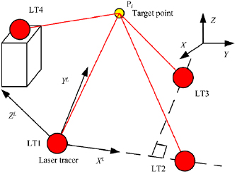
Figure 1. Schematic of four-station laser tracer measurement principle.
Download figure:
Standard image High-resolution image2.2. Self-calibration algorithm of laser tracer
As shown in figure 1, the station LT1  was set as the ordinate origin of the self-calibration coordinate system. Placing the LT2
  on the X-axis, the LT3
  was located in the XY plane, and LT4
  was located at a position that is not coplanar with the plane of the first three stations. The distance between the four laser tracers and the moving target point
  (
( ) can be expressed as
where li (i = 1, 2, 3, 4) is the dead-path length and lij is the measured length of the laser tracer i. The variation of the relative distance between the base station i and the measuring point is defined as 'dead-path length'. The distance between the base station i and initial measuring point j is defined as 'measured length'.
The above equations can be simplified as the matrix linear equations using the first-order approximation of Taylor's expansion:

wherein V is the residual error of equations, A is the coefficient matrix of first-order Taylor's expansion, δX is the variation of the measured unknown parameter, and L is the matrix of measured length.
Because sufficient target positions were measured, equation (2) can be solved using the Levenberg–Marquardt method, and the iterative solution of each step can be written as follows:

where the µ is the relaxation factor.
The calculated positions of laser tracers were among the rotary table coordinates; hence, the coordinate conversion process was needed. The processes of conversion from rotary table to laser tracer coordinates was as follows. Mutual positional relationships of the laser tracer coordinates OLXLYLZL and the rotary table coordinate OXYZ was shown in figure 2.  are the unit vectors of the X, Y, and Z axes of the rotary table coordinates, respectively, and
  are the unit vectors of the XL, YL, and ZL axes of the laser tracer coordinates, respectively. Therefore, the rotational transfer matrix R and the translational transfer matrix T can be written as
wherein
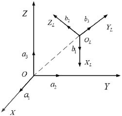
Figure 2. Conversion between self-calibration and rotary table coordinate system.
Download figure:
Standard image High-resolution image is the vector between two coordinate origins O and OL.
Therefore, the coordinate conversion matrix can be given as

The expression of the laser tracer coordinate transform can be given as

2.3. Measuring point solving algorithm
As the self-calibration process was completed, the positions (xpi, y pi, zpi) (i = 1, 2, 3, 4) of the four laser tracer were located in the designated coordinate system; hence, only the coordinates of the target points and the length of the dead-path were unknown. Upon building the objective function Fc based on a distance equation between the target position and laser tracer position for the measured point j , equations (7) and (8) could be obtained as follows:
where j (j = 1, 2, 3..., n) is one measured target position.
The above equations can be solved using the Levenberg–Marquardt method, also, and the singular problems of the nonlinear equations can be avoided. As the positions of laser traces were known according to the algorithm, the existence of the solution could be ensured; hence, the selection of the initial value could be relaxed.
The volumetric error of the measured point (Δxj , Δy j , Δzj ) could be obtained after the theoretical value was calculated, and it can be expressed as
where (xj , y j , zj ) is the actual spatial coordinate of the j th measured point, and  is the ideal coordinate.
The ideal coordinate of the measured point should be known before performing the calculation of volumetric error of the target point. In the process of geometric error measurement of the rotary table, the measured point was fitted as the theoretical measured radius, and the theoretical point coordinates were drawn in accordance with equation (5).
3. Geometric error modeling and separation of rotary table
There are six geometric errors related to the position of the NC rotary table. Considering axis C as an example, ECC is the angular positioning error of axis C, EBC is the tilt error motion of axis C around the Y axis, EAC is the tilt error motion of axis C around the X axis, EZC is the axial error motion along the Z direction of axis C, EXC is the radial error motion of axis C in the X direction, and EYC is the radial error motion of axis C in the Y direction.
According to the screw theory, the ideal position of the rotary table is established as follows:

where  is the ideal orientation of the rotary table,
  is the rigid body motion transformation matrix, and gCst(0) is the initial orientation of the rotary table.
The actual position of the rotary table can be obtained considering the six geometric errors related to the positions of the rotary table:

It can also be represented by
where the Re is the actual pose and Te is the actual position of rotary table.
The geometric error of the rotary table is equal to the difference between the ideal and actual orientations of the rotary table. Using the product exponentials formula, the orientation and position error of the rotary table can be obtained as

where (Xt, Yt, Zt,) is the position of the target retro-reflector (cat's eye) on the rotary table.
The separation of the six geometric errors on the rotary table can be achieved using the spatial position error at three points on the rotary table without collinearity. The measurement schematic is shown in figure 3. Three initial points, Q, M, and K, were selected, and the corresponding volumetric errors were captured during the rotation of the table. Then, the six geometric error items on a specific angle could be calculated by solving the simultaneous equations at the three points. The geometric error formula of each point can be obtained as follows:
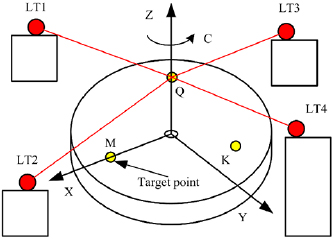
Figure 3. Schematic of geometric error measurement.
Download figure:
Standard image High-resolution imageEquation (15) can also be represented by

Six geometric errors of a NC rotary table can be obtained by using a linear least squares method:

4. Geometric error measurement experiment of NC rotary table
The geometric errors of a hydrostatic NC rotary table were measured using the four-station laser tracers, and the six geometric errors of the NC rotary table were obtained. The experimental results were compared with the radial and axial runouts obtained from the standard ball measurement method and the positioning error measured by the laser interferometer.
4.1. Self-calibration experiment
The four-station laser tracers were used to detect the geometric errors of the horizontal hydrostatic rotary table under an environment of 20 ± 2°. The hydrostatic rotary table has a maximum machining diameter of 240 mm. There was no positioning error compensation for the rotary table. During the measurement process, the laser tracer was first self-calibrated, while the target retro-reflector was placed on the end face of the rotary table and the beam of the interferometer of the laser tracer was moved to the target retro-reflector. Then, the target measurement points were determined at intervals of 10°, and the table was rotated once for measurement, employing a standstill of 3 s at each point. After the measurement was completed, the beam was kept between the laser tracer and the target retro-reflector without interruption, and the target retro-reflector was placed at distances of 80, 160, and 240 mm from the end face of the rotary table, using a processed steel rod. The above steps were repeated to record a rotation measurement, paying special attention to lock the constant beam between the laser tracer and the cat's eye during the whole measurement, as shown in figure 4. After the measurement was obtained, the unknown parameters of the laser tracer were calculated using the calibration method, as shown in table 1. A step-by-step approach for self-calibration experiment is given in figure 5.
Table 1. Laser tracer position system parameters after self-calibration.
| Parameter calibration |  |
 |
 |
 |
 |
 |
|---|---|---|---|---|---|---|
| Calibrated value (mm) | 300.3517 | 511.6718 | −398.9578 | 250.4172 | −633.7587 | 141.6295 |
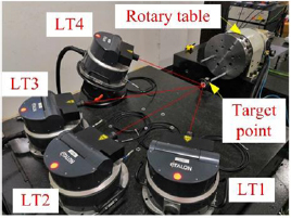
Figure 4. Schematic of self-calibration experiment of laser tracer.
Download figure:
Standard image High-resolution image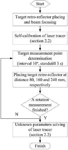
Figure 5. Flow for self-calibration experiment.
Download figure:
Standard image High-resolution image4.2. Experiment for measuring six geometric errors
After the calibration was completed, the four-station laser tracers were kept stationary, and the target retro-reflector (cat's eye) was placed 80 mm away from the end face of the rotary table. The target positions could be measured, and the geometric errors of the rotary table were separated according to the three-point measurement method. While obtaining the measurement, the target retro-reflector was placed on the rotary table with three non-collinear points representing the initial position, and it was assumed that the angular interval between each set of two target retro-reflectors was 120°, which was achieved by rotating the table so as to ensure that the three initial points were on the same circle. According to the established measurement procedure, the rotary table was to rotate counterclockwise at a speed of 1 rpm, and the angular interval between each two determined target measurement points was to be 10°, with 36 points per circle (0–350°) and a standstill of 3 s employed at each measurement position. The coordinates of the initial three points Q, M, and K were measured as shown in table 2, and the results of the measurement process are shown in figures 6 and 7.
Table 2. Measured coordinates of Q, M, and K.
| Measured points | Coordinate | ||
|---|---|---|---|
 (mm) (mm) |
 (mm) (mm) |
 (mm) (mm) |
|
| Q | −300.1417 | −692.2255 | −66.9348 |
| M | −344.1159 | −637.0642 | 10.0001 |
| K | −280.4153 | −716.5912 | 32.6319 |
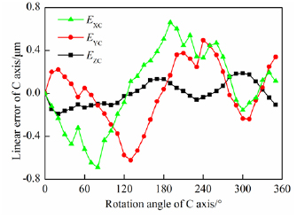
Figure 6. Rotary table linear geometric error.
Download figure:
Standard image High-resolution image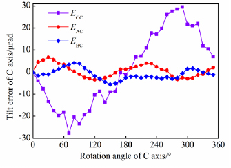
Figure 7. Rotary table angle error.
Download figure:
Standard image High-resolution image4.3. Geometric error comparison experiment
Under the same experimental conditions, a standard ball and micro-displacement sensor were used to measure the axial and radial runouts of the rotary table, as shown in figures 8 and 9. A Tesatronic TT80 Inductance micrometer and a high-precision inductive gauge head (GT21; repeatability 0.01 µm) were used to measure the two runout errors. The standard sphere has a diameter 45 mm and peak-valley value of 40 nm. The comparison between the measurement results obtained using the laser tracer and standard ball is shown in figures 10 and 11. A Renishaw laser interferometer (XL 80) and a rotary axis calibrator were used to measure the positioning error of the rotary table. The experimental setup and the measurement comparison results are shown in figures 12 and 13.
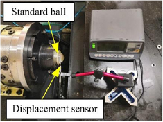
Figure 8. Radial runout measurement of standard ball and micro-displacement sensor.
Download figure:
Standard image High-resolution image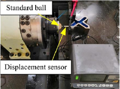
Figure 9. Axis runout measurement of standard ball and micro-displacement sensor.
Download figure:
Standard image High-resolution image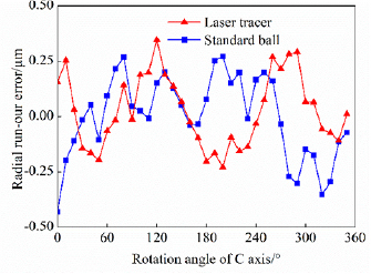
Figure 10. Comparison of radial runout measurement results.
Download figure:
Standard image High-resolution image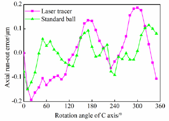
Figure 11. Comparison of axial runout measurement results.
Download figure:
Standard image High-resolution image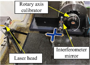
Figure 12. Positioning error measurement by laser interferometer.
Download figure:
Standard image High-resolution image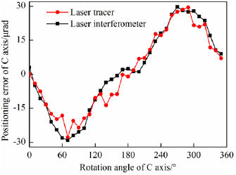
Figure 13. Comparison of positioning error measurement results.
Download figure:
Standard image High-resolution image
A comparison between the measurement results obtained using the laser tracer and conventional method is shown in table 3.
Table 3. Comparison results between laser tracer and conventional test methods.
| Particulars | Results (laser tracer) | Results (standard ball) | Results (laser interferometer) |
|---|---|---|---|
| Journal runout (µm) | 0.70 | 0.62 | — |
| Axial runout (µm) | 0.37 | 0.30 | — |
| Positioning error (µrad) | 57.2 | — | 59.4 |
| Measurement time (h) | 0.5 | 2 | 1 |
From the comparison diagram of radial and axial runouts shown in figures 10 and 11 and the comparison diagram of positioning error in figure 13, it can be concluded that the geometric error measurement method of the rotary table proposed in this study shows a small difference from the results of the conventional rotary precision measurement method, and its trend is very similar. Compared with the standard ball-based method, the radial and axial runout results obtained using the laser tracer show differences of 0.08 and 0.07 µm, respectively. Compared with the results obtained using the laser interferometer, the results of positioning error measurement shows a difference of 2.2 µrad. Because both the standard ball test and the laser interferometer measurement method are affected by installation eccentricity, the centers of the ball rotary axis do not coincide, which leads to deviation of the measurement results. However, the measurement results are similar, which can verify the accuracy of the geometric error measurement method proposed in this study. The laser tracer measurement method is also biased by the influence of the laser tracer layout and its length measurement uncertainty. In addition, it can be seen that the measurement time required by the laser tracer is 0.5 h, which is much less than that required in the standard ball test (2 h) and laser interferometer test (1 h) under the premise of ensuring the measurement accuracy. It is demonstrated that the efficiency improved by five times. The efficiency was defined as the sum of spending time engaged in runout error and positioning error measurement by different methods. Thus, this method demonstrates greater practical and engineering significance.
5. Conclusions
This study proposed a method for the measurement and separation of geometric errors of an NC rotary table, using four-station laser tracers. Self-calibration algorithms for the laser tracers and measuring point solving algorithms were realized for obtaining the volumetric error of the targeted point. Upon integration of the screw theory with the NC rotary table geometric error method, separation of the six item errors was realized via the proposed three-point measurement method.
Compared to the efficiency of the conventional NC rotary table geometric error measurement method, that using the Etalon laser tracer is greatly improved under the premise of ensuring measurement accuracy. The radial and axial runouts show the same trends, and only a small difference by employing two different measurement methods is obtained, which indicates the accuracy and effectiveness of the proposed method. Future work will be conducted on some other rotation axes geometric error measurement, such as a spindle or swing milling head in machining centers.
Acknowledgment
This work was supported by the Fundamental Research Funds for the Central Universities (Grant No. xzy012019007), Shenzhen Science and Technology Project (Grant No. JCYJ20180306170733170), Natural Science Foundation of Jiangsu Province (Grant No. BK20190218), Natural Science Foundation of Shaanxi Province (Grant No. 2018JQ5040), and National Key S&T Special Projects (Grant No. 2018ZX04002001).