

Abstract
Surface dielectric-barrier-discharge (DBD) is widely utilized for flow control actuators called DBD plasma actuator (DBDPA). With the aim of ensuring an accurate background-oriented schlieren (BOS) measurement of the near-surface density field in surface DBD, we investigate the effects of the depth of field (DoF), the wall surface and the background image deformation on measurement results. Experiments using a glass plate as the measurement target reveal that there is no appreciable effect of whether the DoF includes the measurement target. Additionally, the DoF should be shallow from the viewpoint of the error introduced by the wall surface. Moreover, it is found that the error introduced by the wall surface and the dot deformation can be characterized by specific dimensionless parameters. Finally, we conduct the BOS measurement of the DBDPA. We confirm that the density field is qualitatively valid from a physical respect, and we present the density field while discussing specific measurement errors.
Export citation and abstract BibTeX RIS

Original content from this work may be used under the terms of the Creative Commons Attribution 4.0 license. Any further distribution of this work must maintain attribution to the author(s) and the title of the work, journal citation and DOI.
1. Introduction
Over two decades, active flow control devices that use atmospheric discharge have increasingly received attention, with plasma actuators using surface dielectric barrier discharge (DBDPAs) being promising devices (Corke et al 2009, Benard and Moreau 2014). A DBDPA comprises an insulator and two electrodes (figure 1). One electrode is exposed to the air and the other is insulated. Surface barrier discharge is obtained by applying a high AC voltage between the two electrodes. The discharge plasma expands from the top electrode edge along the surface of the DBDPA and manipulates the air flow through interaction with the surrounding air molecules.
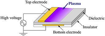
Figure 1. Schematic of a dielectric-barrier-discharge plasma actuator.
Download figure:
Standard image High-resolution imageThe DBDPA has two types of flow control mechanism arising from the discharge. One is the generation of a body force whereas the other is a density fluctuation caused by Joule heating. The former involves the momentum-exchange collision between charged particles accelerated by the Coulomb force and neutral particles, which creates a jet flowing along the wall surface. At the same time, the discharge current causes the Joule heating of the air. It is believed that the body force generation and Joule heating are respectively dominant in flow control when an AC voltage (in the case of AC-DBDPAs) (e.g. Jolibois et al 2008) and nanosecond-pulsed voltage (in the case of NS-DBDPAs) (e.g. Komuro et al 2019a) are applied. The flow control capability of the AC-DBDPA has been demonstrated in many engineering applications for low-velocity flow (Re< 105) owing to the high versatility of the AC-DBDPA (Thomas et al 2008, Audir et al 2016, Matsuda et al 2017, Vernet et al 2018, Shimomura et al 2020). Meanwhile, the NS-DBDPA has better flow separation control capability than the AC-DBDPA for high-speed flow (Re > 106) (Correale et al 2011, Little et al 2012). It is therefore important to understand the body force and Joule heating phenomena of the DBD for the promotion of engineering applications.
Numerous efforts have been made to clarify phenomena of the generation of the body force by measuring the flow velocity, such as particle-image-velocimetry (PIV) (Kotsonis et al 2011, Benard et al 2013, Ota et al 2016, Nakano and Nishida 2019). In contrast, Joule heating has been studied by visualizing the density fluctuation, and almost all relevant studies have made qualitative measurements using, for example, the Schlieren method (Opaits et al 2007, Correale et al 2014). A few recent studies applied the background-oriented schlieren (BOS) technique to the AC-DBDPA and succeeded in quantitatively measuring the density field around the DBD (Biganzoli et al 2015, Komuro et al 2019b). The studies showed that the BOS method is promising but did not discuss the accuracy or reliability of measuring the near-surface density field. It is important to discuss the measurement errors and present guidelines for the accurate measurement of the density field in the vicinity of the surface DBD.
The BOS method is an optical visualization method of quantitatively measuring the density field without contact (Raffel 2015, Hayasaka et al 2016). In the BOS setting, a background image is placed behind the object (i.e. density gradient) as shown in figure 2. The variation in the refractive index due to the density gradient is evaluated on the basis of the displacement of the background image, which can be obtained using a method such as image correlation, which is generally adopted in PIV. Finally, the density field is calculated from the gradient of the refractive index. The BOS method has been used to visualize various flow phenomena because of its simple equipment and measurement procedure (Venkatakrishnan and Meier 2004, Hayasaka et al 2016). There are, however, few examples of the application of the BOS method to the density field of a DBDPA. Here, an example of the BOS measurement of a DBDPA is shown. Figure 3 shows the time-averaged displacement field of the background image over an AC-DBDPA (Kaneko et al 2020). The line y = 0 and origin respectively indicate the plasma actuator surface and the top electrode edge. It can be seen that the displacement vectors spread over the surface and are vertically downward. Three points must be addressed in making a highly accurate BOS measurement of the DBDPA.

Figure 2. Principle of the BOS measurement.
Download figure:
Standard image High-resolution image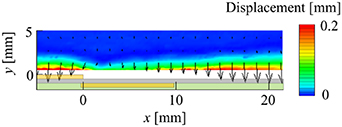
Figure 3. Displacement field of the DBDPA.
Download figure:
Standard image High-resolution imageFirst, we must pay attention to the spatial resolution corresponding to the projection diameter of the cone of light as shown in figure 4. When the equation (1) is satisfied, assuming that the density gradient area can be approximated as a refractive plane, Gojani et al (2013) formulated the spatial resolution δt based on the area of the density gradient where the light rays pass through from the background image pattern as
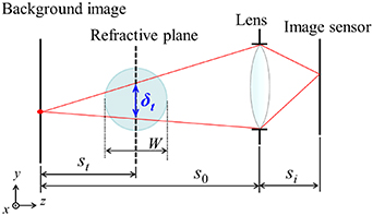
Figure 4. The spatial resolution corresponding to the projection diameter of the cone of light.
Download figure:
Standard image High-resolution imagewhere M = si /s0 is the imaging magnification and f# is the f-number, Δt is the circle of confusion of the image sensor, s0 is the distance between the lens and the background image, si is the distance between the lens and the image plane, st is the distance between the background image and the refractive plane, and l0 is the distance from the background image to the density gradient. Equation (2) indicates that a larger f-number is better for the spatial resolution. Meanwhile, a higher imaging magnification (i.e. higher image resolution) is better for obtaining a fine density distribution, but it reduces the spatial resolution. It is because for obtaining a higher imaging magnification, the camera should be set closer to the background image or the focal length should be increased, that leads to shorter s0. It results in, therefore, larger the diameter of the cone of light on the refractive index plane (see figure 4).
Second, we must pay attention to the effect of the depth of field (DoF). The distance between the background image and the DBDPA l0 should be increased for high measurement sensitivity because of the low density gradient in the DBDPA, and it becomes difficult to keep the DBDPA within the DoF. Two questions arise under such conditions. One is that the object (i.e. the density fluctuation region) is no longer within the DoF. According to Settles and Hargather (2017), both the background image and the measurement object (i.e. the density gradient) should be within the DoF. Klemkowsky et al (2019) investigated the effect of the positional relationship of the DoF, the background image and measurement object on the BOS result in two imaging systems for BOS (i.e. conventional and plenoptic BOS). However, they adopted a buoyant thermal plume as a measurement object, and quantitative effect of the DoF was not discussed because the theoretical value of the result was unknown. In other words, there has been no clear discussion on whether the object should be within the DoF. The other is that the surface of the DBDPA becomes blurry in the captured image. Raffel (2015) said that it is preferable for the dimension of the blur to be much smaller than the interrogation window size. Additionally, Settles and Hargather (2017) concluded that it depends on the researcher whether to accept the blur, and they do not refer to how the blur of the image affect the BOS measurement result. It is not revealed, however, that the effect of the blur of the object on the BOS measurement result near the wall surface. As mentioned above, the displacement vector is directed toward the surface, and the blur of the surface may therefore affect the calculation of the displacement field through image correlation. The present study investigates the density field near the discharge field, and it is thus necessary to clarify how the DoF condition affects the measurement results.
Finally, the deformation of the random-dot image caused by the spatial gradient of the displacement amplitude should be noted because it is considered to greatly affect the accuracy of the image correlation. It can be said that the image deformation is a general problem appearing when there is a spatial gradient in the displacement field and the random-dot image is used as a background image. We need to understand the quantitative effect of image deformation on the calculation of displacement.
The objective of this study is to clarify the BOS settings for the accurate measurement of the DBDPA and to present the density field of the DBDPA while discussing measurement errors. To this end, the effect of the DoF is first investigated using a glass plate as the object, which enables the theoretical calculation of the image displacement. The effect of dot deformation is then investigated using a deformed background image created in image processing. These investigations are conducted with the same measurement settings as for the DBDPA, and the measurement errors attributed to the DoF and dot deformation are identified and parameters characterizing the errors are found. Then, the BOS measurement of the DBDPA is conducted and the results are discussed with the identified errors. In this study, the AC-DBDPA is used as the measurement object because it enables a steady measurement and has been well investigated.
2. Principle of the BOS method
This section presents the measurement principle of the BOS method. The light rays from the background image patterns are deflected owing to the density (refractive index) gradient, resulting in displacement in the background image pattern. In this study, the displacement vectors are obtained through image correlation. Equation (3) (Hinsberg and Rösgen 2014) gives the relation between the displacement vector of the background image pattern U and refractive index n.
Here, W is the thickness of the object with the density gradient, l0 is the distance from the background image to the density gradient, n0 is the refractive index of the air, and C is a correction factor expressed by equation (4). Equation (4) is for the near-field BOS, where 
Using the relationship between the refractive index and density (equation (5), Raffel 2015), equation (3) can be rewritten as equation (6). Here, K is the Gladstone–Dale constant,  is the density of the object and ρ0 is the density of the air.

Finally, by differentiating both sides of equation (6) in space, we obtain Poisson's equation for the density in equation (7). In the BOS method, we obtain the density field by solving equation (7).
3. Measurement accuracy of the BOS method
3.1. Effects of the DoF
3.1.1. Experimental method.
An experiment is conducted for various DoFs by varying the f-number f#. The experimental setup is shown in figure 5. In this experiment, a glass plate is used as a measurement target to enable the theoretical calculation of the displacement vector. The tilt angle of the glass plate is changed, and the experiment is conducted for different magnitudes of displacement. The theoretical value of the displacement is obtained using the equation (8). Here, t (1 mm) is the thickness, nglass (1.52) is the refractive index, and θ is the tilt angle of the glass plate.
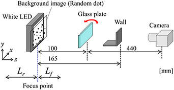
Figure 5. Experimental setup for investigation of the DoF effects.
Download figure:
Standard image High-resolution imageThe aluminum frame material is placed between the glass plate and the camera to simulate the wall surface. Note that, although not only the DoF but also the spatial resolution changes with the f-number as in equation (2), the effect on the spatial resolution does not have to be considered in this experiment because the displacement field is spatially uniform.
The experimental conditions are summarized in table 1. Lr and Lf in figure 5 and table 1 respectively denoted the forward and rear DoF. The experiment is conducted with two different imaging resolutions by changing the focal length f of the lens. A single-lens camera (Nikon D3200) is equipped with a Nikon AF-S DX NIKKOR 18–55 mm f/3.5–5.6 G VR and Nikon AI Micro-Nikkor 105 mm f/2.8 s for low-resolution (0.072 mm/pixel) and high-resolution (0.013 mm/pixel) imaging, respectively.
Table 1. Experimental conditions for low- and high-resolution imaging.
| f-number f# (-) | Focal length f (mm) | Imaging resolution (mm/pixel) | DoF (mm) | |
|---|---|---|---|---|
| Lr | Lf | |||
| Low resolution | ||||
| f/25 | 24 | 0.072 | 544 | 180 |
| f/22 | 427 | 165 | ||
| f/18 | 305 | 143 | ||
| f/13 | 190 | 111 | ||
| f/4 | 47 | 40 | ||
| High resolution | ||||
| f/32 | 105 | 0.013 | 18 | 17 |
| f/16 | 9 | 8 | ||
| f/8 | 4 | 4 | ||
| f/4 | 2 | 2 | ||
The background image is a random-dot pattern, and the dot size is changed with the imaging resolution; i.e. the dot diameter for low- and high-resolution imaging is about 5.7 and 9.4 pixels, respectively. In the low-resolution imaging, both the glass plate and background images are within the DoF except for an f-number of f/4. In high-resolution imaging, the glass plate is not within the DoF under any condition (i.e. only the background image is within the DoF). The tilt angle of the glass plate is changed from −60° to 60° in step of 10°. Table 2 gives image correlation conditions for calculating the displacement. The image correlation algorithm is the same, but the displacements are calculated with different (initial and final) interrogation window sizes to investigate the effect of the window size.
Table 2. Image correlation conditions for calculating the displacement.
| Image correlation algorithm | Interrogation window size (pixel) | Overlap (%) | |
|---|---|---|---|
| Initial | Final | ||
| Low resolution (0.072 mm/pixel) | |||
| Multi-Grid interrogation Multiple correlation Image deformation correlation | 192 | 16 | 50 |
| 96 | 16, 8 | ||
| 64 | 16 | ||
| 32 | 16 | ||
| High resolution (0.013 mm/pixel) | |||
| Multi-Grid interrogation Multiple correlation Image deformation correlation | 256 | 128, 64, 32, 24 | 50 |
| 192 | 32 | ||
| 128 | 32 | ||
| 96 | 32 | ||
3.1.2. Results and discussion.
The effect of DoF is first examined in the area far from the surface (i.e. without the effect of the wall surface). Figure 6 plots the deviation (error) of the displacement from the theoretical value as a function of the tilt angle of the glass plate. Figures 6(a) and (b) plots the error and relative error, respectively. These results are obtained in the low imaging resolution (i.e. the glass plate is within the DoF except in the case of f/4), and the initial and final interrogation window sizes are respectively set at 96 and 16 pixels. The error is the average value over an area 7 mm × 17 mm. The data plotted in this figure is averaged over four measurement results, and the error bars are from the 1.5 standard error. The open circles indicate the results under the condition that the glass plate is not within the DoF. Figure 6(a) shows that the error is 0.3 pixels at most. It is thought that this error is mainly due to the error in setting the tilt angle of the glass plate (estimated to be less than 0.1°) and sub-pixel interpolation error in the displacement calculation. The overlap of the error bars suggests that the results are unaffected by whether the measurement target is within the DoF. Focusing on figure 6(b), the relative error increases as the tilt angle becomes smaller, and it increases up to 30%. It should be noted that the relative error becomes larger in smaller displacement case because of worse signal-to-noise ratio. Figure 7 plots the result obtained in high-resolution imaging setting. Figures 7(a) and (b) plots the error and relative error, respectively. In this setting, the glass plate is not within the DoF in all f-numbers due to longer focal length. As shown in figure 7(a), it can be observed that the error is larger than that in low-resolution imaging setting. It is considered that the error caused by the experimental setting error becomes larger in a higher resolution imaging setting. In contrast, the relative error is less than several % for every tilt angles. This is because the order of the magnitude of the displacement error remains the same, but the theoretical value of the displacement increases in higher imaging resolution setting.
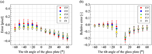
Figure 6. Errors in displacement in the area far from the wall surface obtained in low-resolution imaging. Open circles for f/4 indicate the condition in which the glass plate is not within the DoF. The error bars show the 1.5 standard error: (a) error and (b) relative error.
Download figure:
Standard image High-resolution image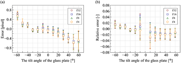
Figure 7. Errors in displacement in the area far from the wall surface obtained in high-resolution imaging. Open symbols indicate the condition in which the glass plate is not within the DoF. The error bars show the 1.5 standard error: (a) error and (b) relative error.
Download figure:
Standard image High-resolution imageWe next show the effect of the wall surface on the displacement calculation. Figure 8 presents the x-profile of the error in 60° tilt angle of the glass plate. The wall surface is at x = 0 mm in this figure, and the left and right axes respectively indicate the error and relative error. The plotted values are averaged along the y-direction, with the error bars showing the 1.5 standard error from four measurement results. Noted that the averaged value of the error in the area far from the wall surface is subtracted for simply showing the effect of the wall surface. Figures 8(a) and (b) show the result in low- and high-resolution imaging setting, respectively. The open symbols in these figures indicate that the wall surface is not within the DoF. As shown in figure 8(a), the errors in the condition with large f-numbers (i.e. a deep DoF) rapidly increase, up to 10% relative error, approaching the wall surface whereas the errors are small in smaller f-number cases (i.e. a shallow DoF). In other words, the error introduced by the wall surface can be greatly reduced when the wall surface is not within the DoF. In this experiment, the displaced dot pattern near the wall surface is hidden behind the image of the wall surface. This is considered to reduce the accuracy of image correlation. Here, when the f-number is small (i.e. a shallow DoF) and the wall surface is a blur in the captured image, some dots hidden behind the wall become visible owing to the blur of the wall surface, which reduces the error in the displacement calculation. Next, focusing on figure 8(b) obtained in the high-resolution imaging setting, the error becomes slightly larger approaching the wall surface even in the case of smaller f-number. The smaller f-number results in worse (larger) spatial resolution as shown in equation (2). It is therefore considered that the area of the spatial resolution includes the wall surface, and it causes the displacement calculation error.
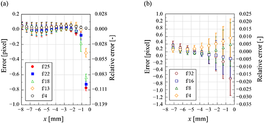
Figure 8. Displacement error profile from the wall surface obtained in (a) low-resolution imaging and (b) high-resolution imaging. Open symbols indicate the condition in which the wall surface is not within the DoF. The error bars show the 1.5 standard error.
Download figure:
Standard image High-resolution imageHowever, it should be noted that the error introduced by the wall surface in the high-resolution imaging setting is less than 5%. It can be therefore concluded that although both a blur of the wall surface and the spatial resolution affects the displacement calculation near the wall surface, the effect of the former is dominant.
A dimensionless parameter that expresses the error due to the wall surface is derived in the following. Figure 9 is a schematic figure of the positional relationship between the interrogation window (drawn in red) and the wall. Figures 9(a) and (b) respectively shows the state before and after the dot pattern is displaced by u toward the wall. The distance d in the figure is the range of the background image that becomes visible with the blurring of the wall. Hereafter, we refer to this distance as the blur length. When the image in the interrogation window whose center is at a distance  from the wall surface moves by u larger than
  −WS/2, the interrogation window after the displacement is partially or fully hidden behind the wall, resulting in an error in calculating the displacement. Here, WS is the final interrogation window size. Considering the blur length d, when equation (9) is satisfied, it is expected that the wall does not appreciably affect the results of the displacement calculation.
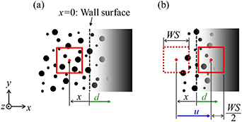
Figure 9. Blurring of the wall surface, image displacement and interrogation window: (a) before image displacement and (b) after image displacement by u toward the wall.
Download figure:
Standard image High-resolution imageThe blur length d can be calculated from the optical diagram. Figure 10 is an optical diagram of the experiment, where A is the aperture of the lens, sw is the distance between the wall and background image, s0 is the distance between the lens and background image, and dw is the distance between the wall surface and optical axis. From the geometric relationship, the blur length d, at which the image hidden behind the wall becomes visible owing to the blur of the wall surface, can be expressed by equation (10).
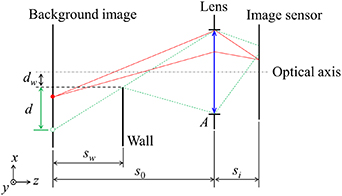
Figure 10. Optical diagram for calculation of the blur length.
Download figure:
Standard image High-resolution imageFigure 11(a) shows plots of the errors against the dimensionless parameter on the left-hand side of equation (9) (hereafter, denoted Dwall ) for all conditions of the tilt angle of the glass plate, f-number, interrogation window size and imaging resolution. Only the condition of the f-number is identified by the plot color and mark type. The red and blue markers indicate the low- and high-resolution imaging cases, respectively. The error on the vertical axis is on a real scale of millimeters. Enlarged graph, figure 11(b), is also shown to make it easier to confirm the result in the high-resolution imaging cases (noted that the results for the low-resolution imaging cases are not plotted in figure 11(b)). Figure 11(a) shows that all the results lie on a single curve. When the dimensionless parameter Dwall on the horizontal axis exceeds zero, the error linearly increases with Dwall . Focusing on figure 11(b), it is observed that the errors in the high-resolution imaging cases also show the linearly increasing trend for Dwall > 0.
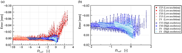
Figure 11. Errors for all measurement settings. The error bars show the 1.5 standard error: (a) full view and (b) enlarged view.
Download figure:
Standard image High-resolution imageIt is concluded that the error due to the wall surface can be suppressed by a larger blur length d (equation (10)) and estimated using the dimensionless parameter Dwall . In other words, the BOS measurement should be conducted while paying attention to Dwall . Figure 11 is obtained with the same BOS settings used for the measurement of the DBDPA described later, and it is expected that the curve in figure 11 can be applied to the measurement of the DBDPA.
3.2. Effects of background image deformation
3.2.1. Analysis method.
Figure 12 shows the procedure used to create the distorted background images used in this analysis. First, background image A acquired under the high-resolution imaging setting (0.013 mm/pixel) is deformed by applying a displacement distribution to the image in image processing. The displacement distribution is uniform in the x-direction and has a constant spatial gradient in the y-direction. Image B is thus obtained. The displacement field is then calculated from images A and B through image correlation. The y-directional profile of the displacement is obtained by averaging the displacement along the x-direction. By comparing the y-directional profile with the given displacement distribution, we discuss the error due to the dot deformation. In this study, five spatial gradients of the displacement distribution are investigated: 0.1, 0.2, 0.3, 0.4 and 0.5. The conditions of image correlation are summarized in table 3.
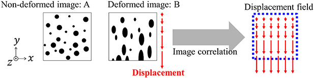
Figure 12. Image processing for investigation of the background image deformation effect.
Download figure:
Standard image High-resolution imageTable 3. Image correlation conditions for calculating the displacement.
| Image correlation algorithm | Interrogation window size [pixel] | Overlap [%] | |
|---|---|---|---|
| Initial | Final | ||
| Multi-Grid interrogation Multiple correlation Image deformation correlation | 256 | 48 | 50 |
| 32 | |||
| 96 | 48 | ||
| 32 | |||
3.2.2. Results and discussion.
The analysis confirms that the error increases for a larger spatial gradient of the displacement. This is a reasonable result because the deformation rate of the random dots increases. The error also increases with the magnitude of the displacement. Additionally, the error increases when the interrogation (final) window size WS decreases. This is because the effect of the deformation increases relatively. On the basis of the above results, the error is plotted as a function of the parameter Dd = (v× dv/dy)/WS for all conditions in figure 13. Here, v is the displacement. The condition of the spatial gradient of the displacement is identified by the marker type, and the interrogation window size is identified by the plot color. The error bars show the 1.5 standard error. The error and error bars are greater for Dd larger than 0.2. It is thus concluded that Dd should be less than 0.2.
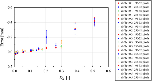
Figure 13. Errors due to dot deformation. The error bars show the 1.5 standard error.
Download figure:
Standard image High-resolution image3.3. Discussion on the BOS measurement of the DBDPA
The above results and discussion show that it is preferable to take images under shallow-DoF conditions from the viewpoint of errors due to the wall surface as discussed in the section 3.1. Therefore, higher-resolution imaging should be adopted because it leads to a shallow DoF as shown in table 1. It is preferable also from the viewpoint of obtaining the near-surface density field.
Here, the discussion on the BOS measurement settings is made focusing on the measurement resolution of displacement field. It is limited by the worse of the resolution of that the displacement vector is calculated (calculation resolution) or the spatial resolution δt . The calculation resolution of displacement vector is determined from the interrogation window size and imaging resolution. On the other hand, the spatial resolution changes depending on the f-number and imaging resolution. Figure 14 plots the calculation resolution of displacement vector for several interrogation window sizes and the spatial resolution for several f-numbers as a function of the focal length (i.e. the imaging resolution). The calculation resolution of displacement vector increases with increases in the focal length and with decrease in the interrogation window size. Focusing on the spatial resolution, it increases with decrease in the focal length and with increase in the f-number. That is, there is a trade-off relation between the calculation resolution of displacement vector and spatial resolution. In addition, change in the f-number affect not only the spatial resolution but also the error due to the wall surface. The larger f-number (decrease in aperture) leads to decrease in the blur length d and it increases the error introduced by the wall surface (see figure 8). There is, therefore, a trade-off relation between the spatial resolution and the error introduced by the wall surface. We must pay careful attention to these relations. It can be concluded that the f-number should be larger for the improvement of the spatial resolution while keeping the error introduced by the wall surface at small level.
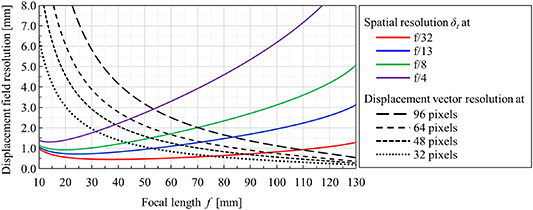
Figure 14. Spatial resolution δt and displacement vector resolution versus focal length f.
Download figure:
Standard image High-resolution imageFrom the above discussions, for obtaining the fine density field of near-surface region, the focal length is set to be 105 mm (i.e. highest imaging resolution setting in this experiment, 0.013 mm/pixel). In this imaging resolution, shallower DoF is achieved even if the larger f-number, so larger f-number, f/32, is adopted from the viewpoint of the spatial resolution. As discussed in section 3.1, the error due to the wall surface in this imaging setting (i.e. 0.013 mm/pixel and f/32) is negligibly small. The interrogation window size therefore should be smaller than 96 pixels from the viewpoint of the measurement resolution of displacement field (see figure 14).
4. BOS measurement of the DBDPA
4.1. Experimental method
Figure 15 is a schematic of the BOS setting for the DBDPA. The arrangement of the LED, background image, camera and measurement target is the same as that in section 3. A Nikon AI Micro-Nikkor 105 mm f/2.8 s is used in this experiment for high imaging resolution (0.013 mm/pixel) and the f-number is set at f/32, at which the DBDPA is not within the DoF as shown in figure 15. The time-averaged density field is obtained from 60 images. The DBDPA is driven by a high voltage amplified by a high-voltage power supply (Trek Model20/20 C-HC). The AC voltage waveform is sinusoidal and the AC frequency is fixed at 2 kHz. The applied voltage is varied as 8, 10 and 14 kVpp. The DBDPA used in this study is a reference plasma actuator made by the National Institute of Advanced Industrial Science and Technology. The DBDPA comprises a silicon resin dielectric plate with thickness of 0.4 mm and two copper electrodes with thickness of 0.018 mm, and has a span length of 100 mm. The image correlation conditions are given in table 4. The size of the final interrogation window is set at 48 pixels to reduce the error due to the dot deformation. Note that the overlap of the interrogation window is set at 80% to increase the displacement vector density. Here, the spatial resolution is mentioned. The spatial resolution δt is calculated from the imaging conditions to be about 0.8 mm using equation (2). In contrast, the resolution calculated from the imaging resolution and interrogation window size is about 0.6 mm. The actual resolution of the displacement field is therefore 0.8 mm.
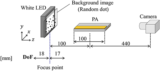
Figure 15. Schematic of the BOS setting for the DBDPA.
Download figure:
Standard image High-resolution imageTable 4. Conditions of image correlation for calculating the displacement.
| Interrogation window size (pixel) | |||
|---|---|---|---|
| Image correlation algorithm | Initial | Final | Overlap (%) |
| Multi-Grid interrogation Multiple correlation Image deformation correlation | 96 | 48 | 80 |
The density field is obtained using the method proposed by Komuro et al (2019b). Equation (7) is solved thorough successive over-relaxation. The acceleration factor is set at 1.9. The iterative calculation is continued while the relative error is larger than 10−8. The boundary condition at the surface of the DBDPA is obtained using the integral solution. Specifically, spatial integration along −y direction of the y-direction component of equation (6).
4.2. Results and discussion
Figure 16 shows the displacement field (left) and density field (right) under three applied voltage conditions.
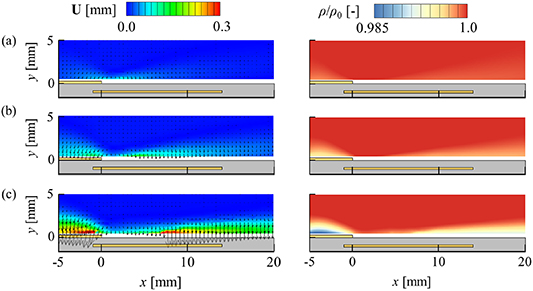
Figure 16. Time-averaged displacement (left column) and density (right column) fields induced by the DBDPA for three applied voltages: (a) 8 kVpp, (b) 10 kVpp and (c) 14 kVpp.
Download figure:
Standard image High-resolution imageWe first focus on the qualitative characteristics of the density field. Under all conditions, the density decreases above the top electrode and dielectric. The discharge occurs at the top electrode edge, where both the flow acceleration due to the body force and the Joule heating caused by the discharge appear. The air flowing into the discharge region is heated, and the heated air then expands during downstream advection over the dielectric surface. This results in an area of lower density spreading along the dielectric surface (spreading more with height in the more downstream region). It is considered that the density change above the top electrode is caused by the heating of the top electrode due to heat transfer from the hot air heated by the discharge. Under the above physical considerations, the density field obtained by the BOS measurement is expected to be qualitatively valid, and the same over all characteristics of the density field were reported in the previous study of Komuro et al (2019b).
We next explain the process for estimating the error included in the displacement field. We first consider the error due to the wall surface and background image deformation. Dwall and Dd are calculated using the vertical displacement v, distance from the surface of the DBDPA, blur length d and (final) interrogation window size WS. Note that, sw used for calculation of the blur length d is the length between the background image and the end face of the DBDPA which is closer to the background image, 35 mm. The peak values of Dwall and Dd in each applied voltage conditions are shown in table 5. The errors are then estimated from figures 11 and 13. It is noted that the error bars in figures 11 and 13 are not considered. Additionally, the measurement error that is less than 1 pixel as shown in figure 7 is included in the displacement value. Furthermore, the uncertainty derived from the repeated measurements (60 images) is considered. The combined value of the above mentioned errors is assumed to appear as positive and negative error, and the uncertainty in the density is finally calculated by the propagation of this combined error.
Table 5. The peak values of Dwall and Dd in each applied voltage conditions.
| 8 kVpp | 10 kVpp | 14 kVpp | |
|---|---|---|---|
| Dwall | −0.11 | 0.43 | 1.52 |
| Dd | 0.04 | 0.18 | 1.17 |
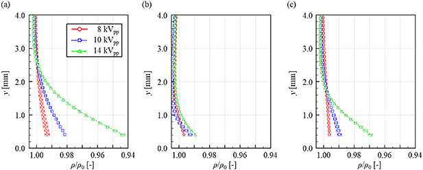
Figure 17 shows the y-profiles of the density field at x = −4.1, 5.0 and 15.1 mm. The error bars in the figure show the combined error calculated above. Focusing on the result of (b) x = 5.0 mm, there is no appreciable difference among the three applied voltages. Meanwhile, the density is lower for higher voltage at (a) x = −4.1 mm and (c) x = 15.1 mm. It can be seen that this tendency is remarkable just above the top electrode and downstream rather than in the discharge region. The results indicate that the density is lowest near the surface of the DBDPA under all conditions. This trend does not correspond to that observed in the previous study conducted by Komuro et al (2019b). They showed that the density is a minimum slightly above the surface. It is thought that the difference is due to the effect of the heat transfer from the wall surface jet to the dielectric surface. In the previous study of Komuro et al (2019b), the measurement was conducted only 1000 ms after the actuator was turn on. It is therefore considered that the surface temperature had not yet reached the steady state, and the cooling effect of the near-surface air due to the heat transfer to the surface led to the low density near the surface. Meanwhile, in this study, the measurement was conducted 5 min after the actuator was turned on to obtain a steady-state density field, and it is expected that the cooling effect due to the heat transfer to the surface is weak.
Figure 17. y-profiles of the density field for three applied voltages at (a) x = −4.1 mm, (b) x = 5.0 mm and (c) x = 15.1 mm.
Download figure:
Standard image High-resolution image
5. Conclusion
This present study investigated the effects of the DoF, wall surface and dot deformation for the accurate measurement of the density field of a DBDPA using the BOS method.
First, the effects of the DoF and wall surface were investigated using a glass plate as the measurement target. The DoF was varied by changing the f-number. Additionally, the glass plate tilt angle, imaging resolution and image correlation conditions were varied. It was observed that whether the measurement target is within the DoF or not does not appreciably affect the results. Meanwhile, near the wall surface, if the DoF is deep (i.e. the f-number is large) and the wall surface is not blurred in the captured image, the error introduced by the wall surface is larger. In other words, this error can be reduced with a shallow DoF (i.e. a smaller f-number). Furthermore, it was confirmed that the error introduced by the wall surface depends on the tilt angle of the glass plate (i.e. the magnitude of the displacement toward the wall surface), f-number, interrogation window size and imaging resolution. For these results, the dimensionless parameter Dwall considering the positional relationship of the interrogation window and the blurry wall was derived. It was confirmed that the error introduced by the wall surface can be characterized by Dwall .
Second, the effect of the deformation of the background image was examined through image processing. A deformed background image was created by applying a displacement distribution to the image. The error due to the dot deformation was discussed by comparing the displacement distribution calculated from the deformed image with the given displacement distribution. The result shows that the error due to the dot deformation increases with the displacement and the spatial gradient of the displacement distribution. Moreover, this error increases as the size of the interrogation window decreases. On this basis, the dimensionless parameter Dd was proposed for estimating the error due to the dot deformation. It is concluded that Dd should be less than 0.2.
Finally, from the above discussion, appropriate BOS measurement settings of the DBDPA were considered. We must consider the f-number, spatial resolution and imaging resolution. In this study, it was concluded that an imaging resolution of 0.013 mm/pixel and an f-number of f/32 are preferable. The BOS measurement of the DBDPA was then conducted with the above measurement settings. This experiment was conducted for three applied voltages. It was found that the density was lower above the dielectric surface and the top electrode. A region of lower density spread over the dielectric surface owing to the air flowing through the discharge region. Additionally, it was considered that hot air heated by the discharge heated the top electrode, and the density above the top electrode changed. In conclusion, the density field obtained using the BOS method is expected to be qualitatively valid. Furthermore, the errors due to the wall surface and dot deformation included in this experiment were estimated using Dwall and Dd , respectively. The y-profiles of the density fields considering the error were shown. The results indicate that the density above the top electrode and dielectric surface decreased with an increasing applied voltage. In contrast, there was no appreciable effect of the applied voltage on the density where the discharge occurred.
Acknowledgments
This work was supported by the Japan Society for the Promotion of Science (JSPS) through a Grants-in-Aid for Scientifc Research (19H02062 and 20H00223). The reference plasma actuator (PAK-Ref03) was provided by the National Institute of Advanced Industrial Science and Technology. Y K conducted the experiments and prepared the paper. Y T contributed to the construction of the experimental setup. H N contributed to the direction and writing of the paper.
Data availability statement
All data that support the findings of this study are included within the article (and any supplementary files).
Conflict of interest
Not applicable.