Random walk centrality for temporal networks

Luis E C Rocha; Naoki Masuda

doi:10.1088/1367-2630/16/6/063023

1. Introduction

Random walks of various types are prototypical dynamical processes on networks. Random walk models are not only objects of pure theoretical interest but the study of their dynamics enlightens general properties of diffusive processes. For instance, properties of random walks are tightly connected to those of interacting particle systems such as stochastic opinion formation models [1, 2] and to current flow in electric circuits [3]. Furthermore, random walks have been applied to searching and routing on networks [4–8], detection of network communities [9] and respondent-driven sampling [10, 11]. A particularly successful application is on ranking of nodes. The PageRank algorithm used for ranking websites and other entities is equivalent to the stationary density of a random walk [12, 13]. Other definitions of centrality (i.e. ranking) of nodes in networks on the basis of the random walk have also been proposed [14–18].

Previous research mostly focused on static structures, i.e. snapshots of networks where the links between the nodes are fixed. Nevertheless, various networks in which node ranking is relevant are dynamic, meaning that a link is used only occasionally in time. The structure of the web graph, for instance, is continuously fluctuating with webpages and links being added and removed at every moment [19]. Human interaction networks derived from, for example, face-to-face conversations [20, 21], sexual contacts [22] and email communication [23] are highly dynamic and follow irregular temporal patterns. As a consequence, the respective interaction matrices vary over time, and a static network representation of such systems becomes deficient. Such varying structures, in which the time order of link availability is relevant, are collectively called temporal networks [24] in contrast to aggregate (or weighted static) networks, in which all interactions within a time-window are collapsed into weighted links.

In the present paper, we propose a centrality measure, named TempoRank, for temporal networks on the basis of the random walk. To realize that, we have to formulate and characterize random walks on temporal networks. Previous studies have addressed diverse properties of the dynamics of random walks on temporal networks, for instance, the cover time [25], mean first-passage time [26, 27], the stationary density [27], mixing time [28, 29], conditions for stationarity and ergodicity [30], and properties of the so-called active random walk [31, 32].

However, to apply a random walk centrality measure to real data, we have to understand random walks on real temporal network data. This is non-trivial for at least two reasons. First, available data are ubiquitously non-stationary. Second, with a high temporal resolution, a snapshot of a network at each time is often sparse, which limits possible pathways for random walkers such that the walk has less choices and the entropy of the process can be considerably reduced. By simulating random walk dynamics in real temporal networks, Starnini and colleagues analyzed the coverage and the mean first-passage time of a random walk model on temporal network data. They found that the diffusion was slower on the temporal network in comparison to the aggregate version [33]. In contrast to their work, we are interested in the stationary density of the random walk in the present study. In another study, Ribeiro and colleagues connected temporal network data to the stationary density of the random walk [34]. They obtained the degree (or weighted degree, also called the strength) of the aggregate network from the data to determine the Poissonian node activity of an evolving network model. Temporal and structural patterns beyond those contained in the node degree of the aggregate network, such as the global structure of the aggregate networks and distributions and correlation of interevent times, were ignored. In contrast to [34], we use temporal network data to directly define the pathways for random walkers, as done in [33].

We formulate the random walk under periodic boundary conditions and regard temporal network data as sequences of snapshots, each of which is an observation of a network within a given time window. We use discrete time random walks. A model in continuous time may enhance the realism of the random walk toy model. Nevertheless, careful discussion of the benefits and limitations of each approach is out of the scope of the present article. We adopt discrete time for mathematical convenience and to readily compare the proposed model with previously proposed centrality measures based on random walk. We examine the stationary density of this random walk and argue that the local inflow considered in the so-called effective network, explicitly constructed from the original network, is sufficient for accurately approximating the stationary density, or the centrality, of the nodes in the temporal networks. We also show that the stationary density depends on the sojourn probability, which regulates the tendency of the walker to stay in the current node, and on the temporal resolution of the network data.

2. TempoRank: a temporal random walk centrality

In this section, we define the TempoRank, i.e. the temporal random walk centrality of a node in temporal networks. TempoRank is the stationary density of the random walk under the periodic boundary condition in time. We also discuss the conditions under which the random walk converges to a unique stationary density.

2.1. Temporal networks

A temporal network with N nodes and length T is defined as a sequence of r time snapshots of equal size ${{T}_{w}}=T/r$ . A temporal network data set typically consists of a list of contacts, and a contact is defined by the identities of the two interacting nodes (i, j), the beginning time t of the contact, and sometimes the duration $\Delta t$ of the contact. The number of contacts between nodes i and j that occur in the tth snapshot, i.e. between time $(t-1){{T}_{w}}$ and $t{{T}_{w}}$ , where $t=1,\ldots ,r$ , is denoted ${{w}_{ij}}(t)$ . The N × N adjacency matrix at time t is given by ${\boldsymbol{w}} (t)=({{w}_{ij}}(t))$ . We assume that links are undirected and thus the adjacency matrices are symmetric. However, the matrices may be weighted with link weights restricted to integers if multiple contacts are observed between two nodes during a single snapshot. The aggregate network (sometimes called the static network) is given by $\sum _{t=1}^{r}{\boldsymbol{w}} (t)$ .

2.2. Transition probability

The definition of a transition matrix for temporal networks is non-trivial because it is necessary to determine the transition probability at isolated nodes. In general, some nodes may be isolated in a snapshot even if the aggregate network is connected. This is particularly the case when the time window for defining the snapshot, ${{T}_{w}}$ , is small. We thus assume that the random walker at an isolated node does not move in the corresponding snapshot. We also assume that the random walker does not move with some probability q (i.e. the sojourn probability) if the node is not isolated. A similar idea of lazy random walks was introduced in [34], and the case q = 0 was explored in [33]. When $0<q<1$ , the random walk process converges to the unique stationary density for any temporal network whose aggregate network is connected (see section 2.3 for more on this).

To define the transition probability, we start with the case in which nodes i and j are adjacent and they are not adjacent to any other node at time t. Then, we assume that in this snapshot a walker at i moves to j with probability $1-q$ and stays at i with probability q. Similarly, a walker at j moves to i with probability $1-q$ and stays at j with probability q. If other node pairs ${{i}^{^{\prime} }}$ and ${{j}^{^{\prime} }}$ are adjacent, and ${{i}^{^{\prime} }}$ and ${{j}^{^{\prime} }}$ are not adjacent to any other node at time t, the walkers transit between ${{i}^{^{\prime} }}$ and ${{j}^{^{\prime} }}$ with the same probabilities.

If i is adjacent only to node ${{j}_{1}}$ at time t and node ${{j}_{2}}$ at time $t+1$ , the walker persists to node i after two time steps with probability ${{q}^{2}}$ . On the basis of this observation, we assume that the walker at i does not move with probability ${{q}^{2}}$ in the snapshot in which i is adjacent to ${{j}_{1}}$ and ${{j}_{2}}$ . The walker moves to either ${{j}_{1}}$ or ${{j}_{2}}$ with probability $(1-{{q}^{2}})/2$ . It should be noted that the probability of the move to ${{j}_{1}}$ and ${{j}_{2}}$ is equal to $(1-q)$ and $q(1-q)$ , respectively, when the two contacts (i, ${{j}_{1}}$ ) and (i, ${{j}_{2}}$ ) appear consecutively, not simultaneously. In this case, the temporal order of the two contacts matters because $(1-q)>q(1-q)$ . In contrast, the two probabilities are the same when nodes ${{j}_{1}}$ and ${{j}_{2}}$ are simultaneously adjacent to i.

In general, we define the transition probability from node i to node j at time t as

$\begin{eqnarray}{{B}_{ij}}\left( t \right)=\left\{ \begin{array}{cc} {{\delta }_{ij}} & \left( {{s}_{i}}\left( t \right)=0,1\leqslant j\leqslant N \right), \\ {{q}^{{{s}_{i}}\left( t \right)}} & \left( {{s}_{i}}\left( t \right)\geqslant 1,i=j \right), \\ {{w}_{ij}}\left( t \right)\left( 1-{{q}^{{{s}_{i}}\left( t \right)}} \right)/{{s}_{i}}\left( t \right) & \left( {{s}_{i}}\left( t \right)\geqslant 1,i\ne j \right), \\ \end{array} \right.\end{eqnarray} \tag{ 1 }$

where ${{\delta }_{ij}}$ is the Kronecker delta and

$\begin{eqnarray}&&{{s}_{i}}\left( t \right)\equiv \mathop{\sum }\limits_{j=1}^{N}{{w}_{ij}}\left( t \right)\end{eqnarray} \tag{ 2 }$

is the node strength, i.e. the number of contacts that node i has, at time t. Note that $\sum _{j=1}^{N}{{B}_{ij}}(t)=1$ . The transition matrix at time t is given by ${\boldsymbol{B}} (t)=({{B}_{ij}}(t))$ .

We define an one-cycle transition matrix for the temporal (abbreviated as tp) network as

$\begin{eqnarray}&&{{{\boldsymbol{P}} }^{{\mbox{tp}}}}\equiv \mathop{\prod }\limits_{t=1}^{r}{\boldsymbol{B}} \left( t \right).\end{eqnarray} \tag{ 3 }$

The stationary density of the random walk under the periodic boundary condition is given by the leading eigenvector (corresponding to the eigenvalue equal to unity) of ${{{\boldsymbol{P}} }^{{\mbox{tp}}}}$ . The periodic boundary condition is given by the sequence ..., ${\boldsymbol{w}} (1)$ , ${\boldsymbol{w}} (2)$ , ..., ${\boldsymbol{w}} (r)$ , ${\boldsymbol{w}} (1)$ , ${\boldsymbol{w}} (2)$ , ... and is necessary because of the finite observation time of an empirical temporal network [33]. When $q\approx 1$ , equation (1) is reduced to

$\begin{eqnarray}{{B}_{ij}}\left( t \right)\approx \left\{ \begin{array}{cc} {{\delta }_{ij}} & \left( {{s}_{i}}\left( t \right)=0,1\leqslant j\leqslant N \right), \\ 1-{{s}_{i}}\left( t \right)\epsilon & \left( {{s}_{i}}\left( t \right)\geqslant 1,i=j \right), \\ {{w}_{ij}}\left( t \right)\epsilon & \left( {{s}_{i}}\left( t \right)\geqslant 1,i\ne j \right), \\ \end{array} \right.\end{eqnarray} \tag{ 4 }$

up to the first order of $\epsilon \equiv 1-q\ll 1$ . By combining equations (3) and (4) and neglecting $O({{\epsilon }^{2}})$ terms, we obtain

$\begin{eqnarray}P_{ij}^{{\mbox{tp}}}=\left\{ \begin{array}{cc} 1-s_{i}^{{\mbox{ag}}}\epsilon & \left( i=j \right), \\ \mathop{\sum }\limits_{t=1}^{r}{{w}_{ij}}\left( t \right)\epsilon & \left( i\ne j \right), \\ \end{array} \right.\end{eqnarray} \tag{ 5 }$

where

$\begin{eqnarray}&&s_{i}^{{\mbox{ag}}}\equiv \mathop{\sum }\limits_{t=1}^{r}{{s}_{i}}\left( t \right)=\mathop{\sum }\limits_{t=1}^{r}\mathop{\sum }\limits_{j=1}^{N}{{w}_{ij}}\left( t \right)\end{eqnarray} \tag{ 6 }$

is the node strength in the aggregate (abbreviated as 'ag' in equation (6)) network. Equation (5) is the transition probability of the continuous-time random walk on the aggregate network for infinitesimally small time .

2.3. Mixing property

In the present work, we say that the random walk is mixing if the modulus of the second largest eigenvalue of the corresponding transition matrix, such as ${{{\boldsymbol{P}} }^{{\mbox{tp}}}}$ , is smaller than unity [35]. This property is necessary and sufficient for the convergence of the random walk to a unique stationary density starting from an arbitrary initial density.

The mixing property holds true for $0<q<1$ , if and only if the aggregate network is connected. If the aggregate network is disconnected, trivially the random walk is not mixing. On the other hand, if the aggregate network is connected, there is a path of length ${{L}_{ij}}$ from any node i to any node j in the aggregate network. With a positive probability, a random walker located at i travels on the first link of this path in a snapshot and does not move in all other snapshots in the first cycle of the application of ${{{\boldsymbol{P}} }^{{\mbox{tp}}}}$ . Then, the random walker moves to the neighbor of i on the mentioned path. Similarly, a random walker moves to a next node on the path in the second cycle with a positive probability, and so on. Therefore, the walker moves from i to j after ${{L}_{ij}}$ cycles with a positive probability. In addition, for any $n(\geqslant 0)$ , the walker moves from i to j after ${{L}_{ij}}+n$ cycles with a positive probability by never moving in n of the ${{L}_{ij}}+n$ cycles. Because i and j are arbitrary, ${{({{{\boldsymbol{P}} }^{{\mbox{tp}}}})}^{\ell }}$ is a positive matrix for $\ell ={{{\rm max} }_{i,j}}{{L}_{ij}}$ , i.e. any entry of ${{({{{\boldsymbol{P}} }^{{\mbox{tp}}}})}^{\ell }}$ is positive. Therefore, the random walk is mixing.

Nevertheless, if q = 0, the mixing property is not necessarily satisfied even if the aggregate network is connected. For example, the adjacency matrix of the triangle is a positive matrix such that the random walk on the static triangle network is mixing. However, in the temporal network with r = 3 in which each of the three snapshots contains just one contact, i.e. ${{w}_{12}}(1)={{w}_{21}}(1)={{w}_{13}}(2)={{w}_{31}}(2)={{w}_{23}}(3)={{w}_{32}}(3)=1$ , and all other ${{w}_{ij}}(t)=0$ , the walker starting from node 1 comes back to node 1 with probability one at t = 3. This means that the random walk on the temporal network is not mixing although that on the corresponding aggregate network (i.e. triangle) is. For example, if each node has at most one neighbor in each snapshot, the random walk on the temporal network is not mixing because the walker has to move to a unique destination within each snapshot. This situation typically occurs when the temporal resolution of the data is high and ${{T}_{w}}$ is small. Then, the random walk is periodic and the stationary density does not exist. In particular, if the walker starts from one node, the density is concentrated on a single node at any time. Finally, if q = 1, the walker never moves, and the random walk is not mixing

2.4. Stationary density and the definition of the TempoRank

Assume that the random walk induced by ${{{\boldsymbol{P}} }^{{\mbox{tp}}}}$ is mixing. We denote the unique stationary density of the random walk, i.e. the leading left eigenvector of ${{{\boldsymbol{P}} }^{{\mbox{tp}}}}$ , by

$\begin{eqnarray}&&{\boldsymbol{v}} \left( 1 \right)=\left( {{v}_{1}}\left( 1 \right)\ {{v}_{2}}\left( 1 \right)\ \cdots \ {{v}_{N}}\left( 1 \right) \right),\end{eqnarray} \tag{ 7 }$

where ${{v}_{i}}(1)$ ( $1\leqslant i\leqslant N$ ) is the stationary density at node i. In other words,

$\begin{eqnarray}&&{\boldsymbol{v}} \left( 1 \right)={\boldsymbol{v}} \left( 1 \right){{{\boldsymbol{P}} }^{{\mbox{tp}}}}.\end{eqnarray} \tag{ 8 }$

The normalization is given by $\sum _{i=1}^{N}{{v}_{i}}(1)=1$ .

In fact, ${\boldsymbol{v}} (1)$ is the stationary density when we observe the random walk at t = mr, where m is integer and tends to $\infty$ . In general, the density fluctuates even in the stationary state because we periodically apply different snapshots to move the walker. For example, the stationary density when we observe the random walk at $t=mr+1$ , where $m\to \infty$ , is given by ${\boldsymbol{v}} (2)\equiv {\boldsymbol{v}} (1){\boldsymbol{B}} (1)$ . The long-term stationary density, i.e. that averaged within a cycle, is given by

$\begin{eqnarray}&&{\boldsymbol{\bar{v}}} \equiv \frac{1}{r}\mathop{\sum }\limits_{t=1}^{r}{\boldsymbol{v}} \left( t \right),\end{eqnarray} \tag{ 9 }$

where

$\begin{eqnarray}&&{\boldsymbol{v}} \left( t \right)={\boldsymbol{v}} \left( 1 \right)\prod ^{\prime} =1t-1t{\boldsymbol{B}} \left( {{t}^{^{\prime} }} \right).\end{eqnarray} \tag{ 10 }$

We define ${\boldsymbol{\bar{v}}} =({{\bar{v}}_{1}}\ \cdots \ {{\bar{v}}_{N}})$ as the temporal random walk centrality, abbreviated as the TempoRank.

Similar to the case of the random walk on static networks, ${{\bar{v}}_{i}}$ is also interpreted as the total inflow to node i. In the stationary state, the inflow to node i at time $t=mr+1$ is given by ${{({\boldsymbol{v}} (1){\boldsymbol{B}} (1))}_{i}}={{({\boldsymbol{v}} (2))}_{i}}$ because ${\boldsymbol{v}} (1)$ is the stationary density at t = mr and ${\boldsymbol{B}} (1)$ is the transition matrix at $t=mr+1$ . The inflow to node i at $t=mr+2$ is given by $({\boldsymbol{v}} (2){\boldsymbol{B}} (2))={{({\boldsymbol{v}} (3))}_{i}}$ because ${\boldsymbol{v}} (2)$ is the stationary density at $t=mr+1$ and ${\boldsymbol{B}} (2)$ is the transition matrix at $t=mr+2$ . Same for $t=mr+3,\ldots ,(m+1)r$ . The total inflow of the probability to node i in a cycle is given by ${{({\boldsymbol{v}} (2))}_{i}}+{{({\boldsymbol{v}} (3))}_{i}}+\cdots +{{({\boldsymbol{v}} (r))}_{i}}+{{({\boldsymbol{v}} (r){\boldsymbol{B}} (r))}_{i}}={{({\boldsymbol{v}} (2))}_{i}}+{{({\boldsymbol{v}} (3))}_{i}}+\cdots +{{({\boldsymbol{v}} (r))}_{i}}$ $+{{({\boldsymbol{v}} (1))}_{i}}=r{{\bar{v}}_{i}}$ . Therefore, ${{\bar{v}}_{i}}$ is equal to the average inflow to node i per time step.

The stationary densities ${\boldsymbol{v}} (1)$ and ${\boldsymbol{\bar{v}}}$ depend on the value of q, which contrasts with the results obtained from a different model [34]. The temporal random walk induced by ${{{\boldsymbol{P}} }^{{\mbox{tp}}}}$ coincides with the continuous-time random walk in the aggregate network in the limit $q\to 1$ (equation (5)). Here, we mean by the continuous-time random walk that the hopping rate on each link is equal to unity such that the hopping rate for a node is equal to the nodeʼs degree. In general, the stationary density of the continuous-time random walk in a connected network is given by $1/N$ at each node [36]. Therefore, we obtain ${\boldsymbol{v}} (t)$ $(1\leqslant t\leqslant r)$ , ${\boldsymbol{\bar{v}}} \to (1\ \cdots \ 1)/N$ in the limit $q\to 1$ .

2.5. Random walk on the aggregate network

The transition matrix of the discrete-time random walk on the aggregate network is given by

$\begin{eqnarray}&&{{{\boldsymbol{P}} }^{{\mbox{ag}}}}\equiv {{\left[ \mathop{\sum }\limits_{t=1}^{r}{\boldsymbol{D}} \left( t \right) \right]}^{-1}}\left[ \mathop{\sum }\limits_{t=1}^{r}{\boldsymbol{w}} \left( t \right) \right],\end{eqnarray} \tag{ 11 }$

where the N × N diagonal matrix ${\boldsymbol{D}} (t)$ is defined by ${{D}_{ij}}(t)={{\delta }_{ij}}\sum _{\ell =1}^{N}{{w}_{i\ell }}(t)$ $(={{\delta }_{ij}}\sum _{\ell =1}^{N}{{w}_{\ell i}}(t))$ . The diagonal elements of $\sum _{t=1}^{r}{\boldsymbol{D}} (t)$ are equal to the node strength of the aggregate network given by equation (6).

${{{\boldsymbol{P}} }^{{\mbox{ag}}}}$ is distinct from ${{{\boldsymbol{P}} }^{{\mbox{tp}}}}$ or its weighted versions. For example, $P_{ij}^{{\mbox{tp}}}>0$ if there is a temporal path from i to j whose length is at most r, whereas $P_{ij}^{{\mbox{ag}}}>0$ ( $i\ne j$ ) if and only if i and j are adjacent.

3. The effective network and the in-strength approximation

In this section, we show that the TempoRank is equal to the stationary density of the discrete-time random walk on a static weighted and directed network, which we call the effective network. In other words, we map the random walk on a temporal network into a directed weighted static network. This program apparently sounds trivial owing to the fact that ${{{\boldsymbol{P}} }^{{\mbox{tp}}}}$ is a transition matrix. Here we explicitly construct the effective network from the given sequence of interaction matrices ${\boldsymbol{w}} (1)$ , ${\boldsymbol{w}} (2)$ , .... This relationship allows us to give a new interpretation to the TempoRank and to develop a local approximator.

Under $0\leqslant q<1$ , equation (1) is equivalent to

$\begin{eqnarray}&&{{B}_{ij}}\left( t \right)=\frac{w_{ij}^{^{\prime} }\left( t \right)}{\mathop{\sum }\limits_{\ell =1}^{N}w_{i\ell }^{^{\prime} }\left( t \right)},\end{eqnarray} \tag{ 12 }$

where

$\begin{eqnarray}w_{ij}^{^{\prime} }\left( t \right)=\left\{ \begin{array}{cc} {{\delta }_{ij}} & \left( {{s}_{i}}\left( t \right)=0,1\leqslant j\leqslant N \right), \\ {{s}_{i}}\left( t \right){{q}^{{{s}_{i}}\left( t \right)}}/\left( 1-{{q}^{{{s}_{i}}\left( t \right)}} \right) & \left( {{s}_{i}}\left( t \right)\geqslant 1,i=j \right), \\ {{w}_{ij}}\left( t \right) & \left( {{s}_{i}}\left( t \right)\geqslant 1,i\ne j \right). \\ \end{array} \right.\end{eqnarray} \tag{ 13 }$

In terms of the undirected weighted matrix ${{{\boldsymbol{w}} }^{^{\prime} }}(t)=(w_{ij}^{^{\prime} }(t))$ , we obtain

$\begin{eqnarray}\begin{array}{rcl} P_{ij}^{{\mbox{tp}}} & = & \mathop{\sum }\limits_{{{k}_{1}},\ldots ,{{k}_{r-1}}}\frac{w_{i{{k}_{1}}}^{^{\prime} }(1)}{\mathop{\sum }\limits_{{{\ell }_{1}}}w_{i{{\ell }_{1}}}^{^{\prime} }(1)}\frac{w_{{{k}_{1}}{{k}_{2}}}^{^{\prime} }(2)}{\mathop{\sum }\limits_{{{\ell }_{2}}}w_{{{k}_{1}}{{\ell }_{2}}}^{^{\prime} }(2)}\cdots \frac{w_{{{k}_{r-1}}j}^{^{\prime} }(r)}{\mathop{\sum }\limits_{{{\ell }_{r}}}w_{{{k}_{r-1}}{{\ell }_{r}}}^{^{\prime} }(r)} \\ {} & = & \frac{w_{ij}^{{\mbox{tp}}}(1)}{\mathop{\sum }\limits_{\ell }w_{i\ell }^{{\mbox{tp}}}(1)}, \\ \end{array}\end{eqnarray} \tag{ 14 }$

$\begin{eqnarray}\begin{array}{rcl} P_{ji}^{{\mbox{tp}}} & = & \mathop{\sum }\limits_{{{k}_{1}},\ldots ,{{k}_{r-1}}}\frac{w_{j{{k}_{1}}}^{^{\prime} }(1)}{\mathop{\sum }\limits_{{{\ell }_{1}}}w_{j{{\ell }_{1}}}^{^{\prime} }(1)}\frac{w_{{{k}_{1}}{{k}_{2}}}^{^{\prime} }(2)}{\mathop{\sum }\limits_{{{\ell }_{2}}}w_{{{k}_{1}}{{\ell }_{2}}}^{^{\prime} }(2)}\cdots \frac{w_{{{k}_{r-1}}i}^{^{\prime} }(r)}{\mathop{\sum }\limits_{{{\ell }_{r}}}w_{{{k}_{r-1}}{{\ell }_{r}}}^{^{\prime} }(r)} \\ {} & = & \frac{w_{ji}^{{\mbox{tp}}}(1)}{\mathop{\sum }\limits_{\ell }w_{j\ell }^{{\mbox{tp}}}(1)}, \\ \end{array}\end{eqnarray} \tag{ 15 }$

where

$\begin{eqnarray}&&w_{ij}^{{\mbox{tp}}}(1)\equiv \mathop{\sum }\limits_{{{k}_{1}},\ldots ,{{k}_{r-1}}}\frac{w_{i{{k}_{1}}}^{^{\prime} }(1)w_{{{k}_{1}}{{k}_{2}}}^{^{\prime} }(2)\cdots w_{{{k}_{r-1}}j}^{^{\prime} }(r)}{\mathop{\sum }\limits_{{{\ell }_{1}}}w_{i{{\ell }_{1}}}^{^{\prime} }(1)\mathop{\sum }\limits_{{{\ell }_{2}}}w_{{{k}_{1}}{{\ell }_{2}}}^{^{\prime} }(2)\cdots \mathop{\sum }\limits_{{{\ell }_{r}}}w_{{{k}_{r-1}}{{\ell }_{r}}}^{^{\prime} }(r)},\end{eqnarray} \tag{ 16 }$

$\begin{eqnarray}&&w_{ji}^{{\mbox{tp}}}(1)\equiv \mathop{\sum }\limits_{{{k}_{1}},\ldots ,{{k}_{r-1}}}\frac{w_{j{{k}_{1}}}^{^{\prime} }(1)w_{{{k}_{1}}{{k}_{2}}}^{^{\prime} }(2)\cdots w_{{{k}_{r-1}}i}^{^{\prime} }(r)}{\mathop{\sum }\limits_{{{\ell }_{1}}}w_{j{{\ell }_{1}}}^{^{\prime} }(1)\mathop{\sum }\limits_{{{\ell }_{2}}}w_{{{k}_{1}}{{\ell }_{2}}}^{^{\prime} }(2)\cdots \mathop{\sum }\limits_{{{\ell }_{r}}}w_{{{k}_{r-1}}{{\ell }_{r}}}^{^{\prime} }(r)}.\end{eqnarray} \tag{ 17 }$

In fact,

$\begin{eqnarray}&&\mathop{\sum }\limits_{j=1}^{N}w_{ij}^{{\mbox{tp}}}\left( 1 \right)=1\end{eqnarray} \tag{ 18 }$

holds true for each i such that the denominators of the right-hand sides of equations (14) and (15) are equal to unity.

Equations (14) and (15) indicate that ${{{\boldsymbol{P}} }^{{\mbox{tp}}}}$ is the transition matrix of the discrete-time random walk on the static weighted network defined by ${{{\boldsymbol{w}} }^{{\mbox{tp}}}}(1)=(w_{ij}^{{\mbox{tp}}}(1))$ . We call this network the effective network. In general,

$\begin{eqnarray}&&w_{ij}^{{\mbox{tp}}}\left( 1 \right)\ne w_{ji}^{{\mbox{tp}}}\left( 1 \right).\end{eqnarray} \tag{ 19 }$

Each snapshot ${{{\boldsymbol{w}} }^{^{\prime} }}(t)$ and the aggregate network are undirected networks. However, the concatenation of the different snapshots makes the effective network directed due to the arrow of time, which creates asymmetry in the sequence of link activation.

For static directed networks, the in-degree is often accurate in approximating the stationary density of the random walk [37–41]. Here we develop the same type of local approximation of the TempoRank by considering the in-strength of nodes in the effective network. The in-degree of node i does not generally depend on the out-degree of the upstream neighbors of i. In contrast, the in-strength is large (small) when the out-degree of an upstream neighbor is small (large). The in-strength of node i for the effective network is given by

$\begin{eqnarray}&&s_{i}^{{\mbox{tp}}}\left( 1 \right)\equiv \mathop{\sum }\limits_{j=1}^{N}w_{ji}^{{\mbox{tp}}}\left( 1 \right).\end{eqnarray} \tag{ 20 }$

The in-strength is considered to be an appropriate approximator to the stationary density because equations (8), (14), and (18) imply

$\begin{eqnarray}&&{{v}_{i}}\left( 1 \right)=\mathop{\sum }\limits_{j=1}^{N}{{v}_{j}}\left( 1 \right)w_{ji}^{{\mbox{tp}}}\left( 1 \right)\approx \left\langle v\left( 1 \right) \right\rangle \mathop{\sum }\limits_{j=1}^{N}w_{ji}^{{\mbox{tp}}}\left( 1 \right)=\frac{s_{i}^{{\mbox{tp}}}\left( 1 \right)}{N},\end{eqnarray} \tag{ 21 }$

if all ${{v}_{j}}(1)$ ʼs are approximated by an ensemble average given by $\left\langle v(1) \right\rangle =1/N$ . Equations (19) and (20) imply $\sum _{i=1}^{N}s_{i}^{{\mbox{tp}}}(1)=N$ . Therefore, equation (21) provides a normalized in-strength approximator to ${\boldsymbol{v}} (1)$ .

We calculate the in-strength approximator to ${\boldsymbol{\bar{v}}}$ as follows. Because ${\boldsymbol{v}} (1){{{\boldsymbol{P}} }^{{\mbox{tp}}}}={\boldsymbol{v}} (1){\boldsymbol{B}} (1){\boldsymbol{B}} (2)\cdots {\boldsymbol{B}} (r)={\boldsymbol{v}} (1)$ implies that ${\boldsymbol{v}} (t){\boldsymbol{B}} (t){\boldsymbol{B}} (t+1)\cdots {\boldsymbol{B}} (r){\boldsymbol{B}} (1)\cdots$ ${\boldsymbol{B}} (t-1)={\boldsymbol{v}} (t)$ ( $2\leqslant t\leqslant r$ ), ${\boldsymbol{v}} (t)$ is the stationary density of the random walk in the static network ${{{\boldsymbol{w}} }^{{\mbox{tp}}}}(t)=(w_{ij}^{{\mbox{tp}}}(t))$ defined by

$\begin{eqnarray}&&w_{ij}^{{\mbox{tp}}}(t)\equiv \mathop{\sum }\limits_{{{k}_{1}},\ldots ,{{k}_{r-1}}}\frac{w_{i{{k}_{1}}}^{^{\prime} }(t)w_{{{k}_{1}}{{k}_{2}}}^{^{\prime} }(t+1)\cdots w_{{{k}_{r-1}}j}^{^{\prime} }(t-1)}{\mathop{\sum }\limits_{{{\ell }_{1}}}w_{i{{\ell }_{1}}}^{^{\prime} }(t)\mathop{\sum }\limits_{{{\ell }_{2}}}w_{{{k}_{1}}{{\ell }_{2}}}^{^{\prime} }(t+1)\cdots \mathop{\sum }\limits_{{{\ell }_{r}}}w_{{{k}_{r-1}}{{\ell }_{r}}}^{^{\prime} }(t-1)},\end{eqnarray} \tag{ 22 }$

$\begin{eqnarray}&&w_{ji}^{{\mbox{tp}}}(t)\equiv \mathop{\sum }\limits_{{{k}_{1}},\ldots ,{{k}_{r-1}}}\frac{w_{j{{k}_{1}}}^{^{\prime} }(t)w_{{{k}_{1}}{{k}_{2}}}^{^{\prime} }(t+1)\cdots w_{{{k}_{r-1}}i}^{^{\prime} }(t-1)}{\mathop{\sum }\limits_{{{\ell }_{1}}}w_{j{{\ell }_{1}}}^{^{\prime} }(t)\mathop{\sum }\limits_{{{\ell }_{2}}}w_{{{k}_{1}}{{\ell }_{2}}}^{^{\prime} }(t+1)\cdots \mathop{\sum }\limits_{{{\ell }_{r}}}w_{{{k}_{r-1}}{{\ell }_{r}}}^{^{\prime} }(t-1)}.\end{eqnarray} \tag{ 23 }$

Therefore, the in-strength approximation is given by

$\begin{eqnarray}&&{{\bar{v}}_{i}}\approx \frac{\mathop{\sum }\limits_{t=1}^{r}s_{i}^{{\mbox{tp}}}\left( t \right)}{Nr},\end{eqnarray} \tag{ 24 }$

where

$\begin{eqnarray}&&s_{i}^{{\mbox{tp}}}\left( t \right)\equiv \mathop{\sum }\limits_{j=1}^{N}w_{ji}^{{\mbox{tp}}}\left( t \right).\end{eqnarray} \tag{ 25 }$

4. Numerical analysis

In this section, we numerically examine the TempoRank. We assess the performance of the in-strength approximation on empirical temporal networks and discuss the right moment hypothesis, i.e. the contention that nodes have to contact other nodes at the right moment.

4.1. Data sets

We performed the numerical analysis using the following empirical networks. One network represents face-to-face interactions between conference attendees (SPC) [20], another corresponds to the same type of interactions between visitors to a museum (SPM) [20] and the third to proximity between staff and patients in a hospital (SPH) [21]. The fourth data set corresponds to sexual contacts between sex-sellers and -buyers extracted from a webforum (SEX) [22]. The last data set is a sample of email communication between students and staff within a university (EMA) [23]. These networks represent human interactions in diverse social contexts and have different topological and temporal characteristics (table 1).

Table 1. Summary information about the empirical networks. Number of nodes (N), number of links ( $|E|={{\sum }_{i}}s_{i}^{{\mbox{ag}}}/2$ ), recording time (T), and maximum temporal resolution (δ).

	N	$\|E\|$	T (d)	δ
SPC	113	20 818	∼2.5	20 s
SPM	72	6 980	∼1	20 s
SPH	75	32 424	∼4	20 s
SEX	1302	1 814	50	1 d
EMA	1564	4 461	1	1 s

4.2. Numerical procedures

Consider a given sequence of snapshots $w(1)$ , ..., w(r). We apply the power method on ${{{\boldsymbol{P}} }^{{\mbox{tp}}}}$ (equation (3)) to obtain the stationary density ${\boldsymbol{v}} (1)$ and use equations (9) and (10) to calculate the TempoRank ${\boldsymbol{\bar{v}}}$ . The initial condition is the uniform density ${{{\boldsymbol{v}} }_{{\mbox{init}}}}(1)=(1\ \cdots \ 1)/N$ , and iteration stops when $\sqrt{\mid {{{\boldsymbol{v}} }_{{\mbox{post}}}}(1)-{{{\boldsymbol{v}} }_{{\mbox{pre}}}}(1){{\mid }^{2}}/N}<{{10}^{-6}}$ for the first time, where ${{{\boldsymbol{v}} }_{{\mbox{pre}}}}(1)$ and ${{{\boldsymbol{v}} }_{{\mbox{post}}}}(1)$ are the estimation of ${\boldsymbol{v}} (1)$ before and after multiplying ${{{\boldsymbol{P}} }^{{\mbox{tp}}}}$ , respectively, during the power iteration. The stationary density for the aggregate network, i.e. the normalized leading eigenvector of the transition matrix ${{{\boldsymbol{P}} }^{{\mbox{ag}}}}$ (equation (11)), is given by the (normalized) strength of the node in the aggregate network (equation (6)). This is because the network is undirected [3, 42].

4.3. In-strength approximation

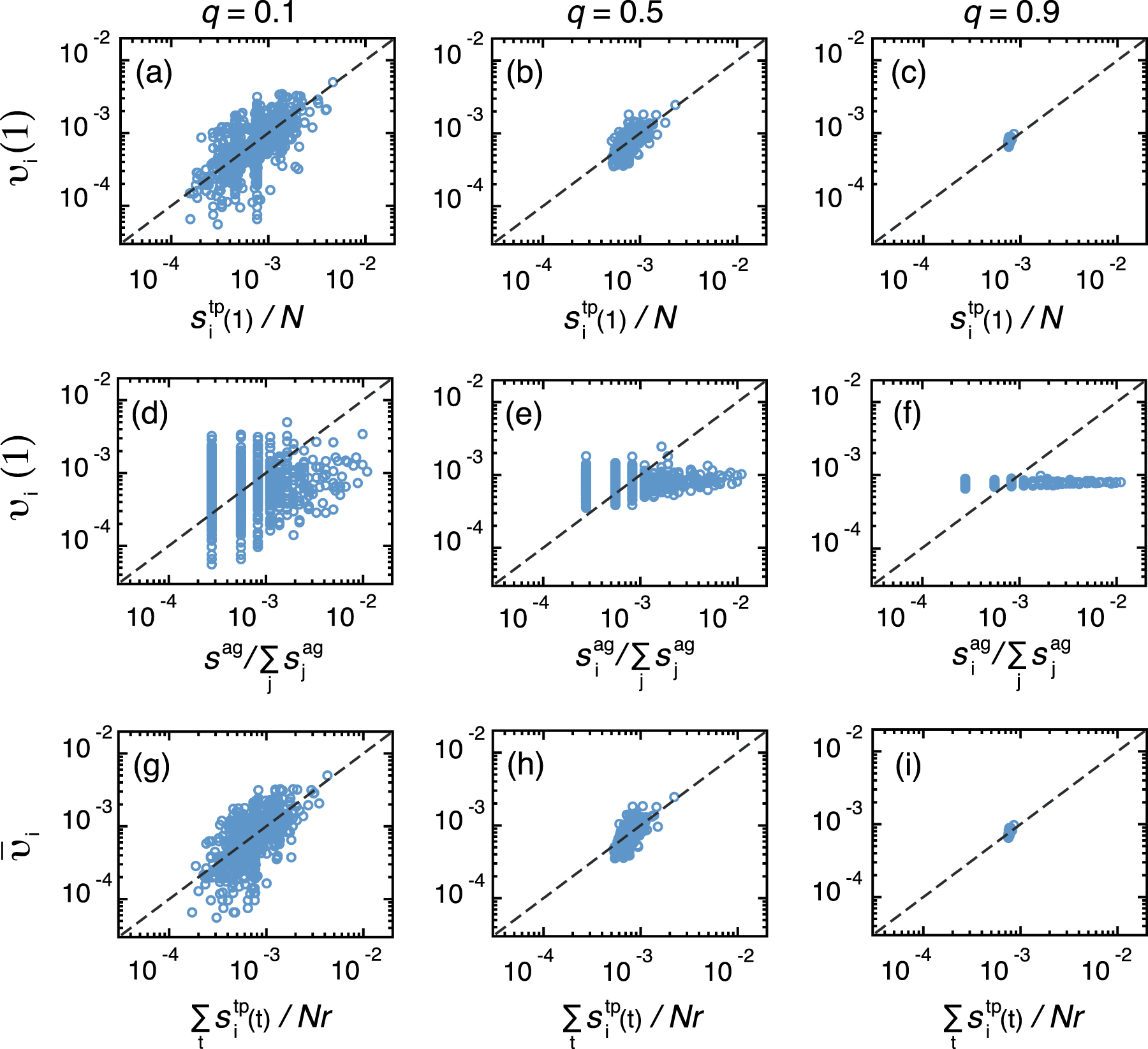
Figures 1(a)–(c) shows the performance of the in-strength approximator with three values of q for the SPC data set. The in-strength approximation is accurate for a wide range of values of q (i.e. from 0.1 to 0.9) for most nodes. In contrast, the in-strength of the aggregate network, i.e. $s_{i}^{{\mbox{ag}}}$ , which gives the exact stationary density of the random walk on the aggregate network, is little correlated with ${{v}_{i}}(1)$ for the same three values of q (figures 1(d)–(f)). The in-strength approximator for the TempoRank (equation (24)) is also strongly correlated with ${{\bar{v}}_{i}}$ , as shown in figures 1(g)–(i). The results are qualitatively the same for the other empirical networks, as shown in figure 2 (for SPM data set) and in the appendix (for the other data sets).

**Figure 1.** TempoRank for SPC network. (a)–(c) Relationship between the stationary density of the temporal transition matrix and the in-strength approximation. Each circle represents a node, and the dashed lines represent the diagonal. (d)–(f) Relationship between the stationary density of the temporal transition matrix and the in-strength of the aggregate network. (g)–(i) Relationship between the TempoRank and the time-averaged in-strength of the effective network. We set q = 0.1 in (a), (d), (g), q = 0.5 in (b), (e), (h) and q = 0.9 in (c), (f), (i). The resolution is ${{T}_{w}}=5$ min.
Download figure:
Standard image High-resolution image

**Figure 1.** TempoRank for SPC network. (a)–(c) Relationship between the stationary density of the temporal transition matrix and the in-strength approximation. Each circle represents a node, and the dashed lines represent the diagonal. (d)–(f) Relationship between the stationary density of the temporal transition matrix and the in-strength of the aggregate network. (g)–(i) Relationship between the TempoRank and the time-averaged in-strength of the effective network. We set q = 0.1 in (a), (d), (g), q = 0.5 in (b), (e), (h) and q = 0.9 in (c), (f), (i). The resolution is ${{T}_{w}}=5$ min.
Download figure:
Standard image High-resolution image

**Figure 2.** TempoRank for SPM network. (a)–(c) Relationship between the stationary density of the temporal transition matrix and the in-strength approximation. (d)–(f) Relationship between the stationary density of the temporal transition matrix and the in-strength of the aggregate network. (g)–(i) Relationship between the TempoRank and the time-averaged in-strength of the effective network. We set q = 0.1 in (a), (d), (g), q = 0.5 in (b), (e), (h) and q = 0.9 in (c), (f), (i). The resolution is ${{T}_{w}}=1$ min.
Download figure:
Standard image High-resolution image

**Figure 2.** TempoRank for SPM network. (a)–(c) Relationship between the stationary density of the temporal transition matrix and the in-strength approximation. (d)–(f) Relationship between the stationary density of the temporal transition matrix and the in-strength of the aggregate network. (g)–(i) Relationship between the TempoRank and the time-averaged in-strength of the effective network. We set q = 0.1 in (a), (d), (g), q = 0.5 in (b), (e), (h) and q = 0.9 in (c), (f), (i). The resolution is ${{T}_{w}}=1$ min.
Download figure:
Standard image High-resolution image

The values of ${{v}_{i}}(1)$ and ${{\bar{v}}_{i}}$ are similar for all nodes when q = 0.9 (figures 1(c), 1(f) and 1(i)). This result is consistent with the theoretical prediction made in section 2.4, i.e. ${\boldsymbol{v}} (1),{\boldsymbol{\bar{v}}} \to (1\ \cdots \ 1)/N$ as $q\to 1$ .

4.4. The right-moment hypothesis

In principle, the stationary density of the random walk at a node is large if the node receives links from nodes with high stationary densities. This principle underlies the design of the PageRank [12, 13]. More generally, the principle that being adjacent to a central node is important, for the node itself to be important, guides the definition of the Katz centrality, eigenvector centrality and their variants [43]. In the case of the TempoRank, however, we show in section 4.3 that the in-strength approximation for the effective network, which ignores the 'next-to-celebrity' principle, is pretty accurate for the particular data sets that we have analyzed.

The 'next-to-celebrity' principle accommodated to the TempoRank dictates that a node i being connected to another node with a large density of walkers at the right moment gains a large inflow at that time, leading to a large ${{\bar{v}}_{i}}$ value. Some centrality measures for temporal networks on the basis of the right-moment principle have been proposed in different forms [44, 45]. Our results in section 4.3 implies that the right-moment principle is practically irrelevant in the TempoRank for the analyzed data sets.

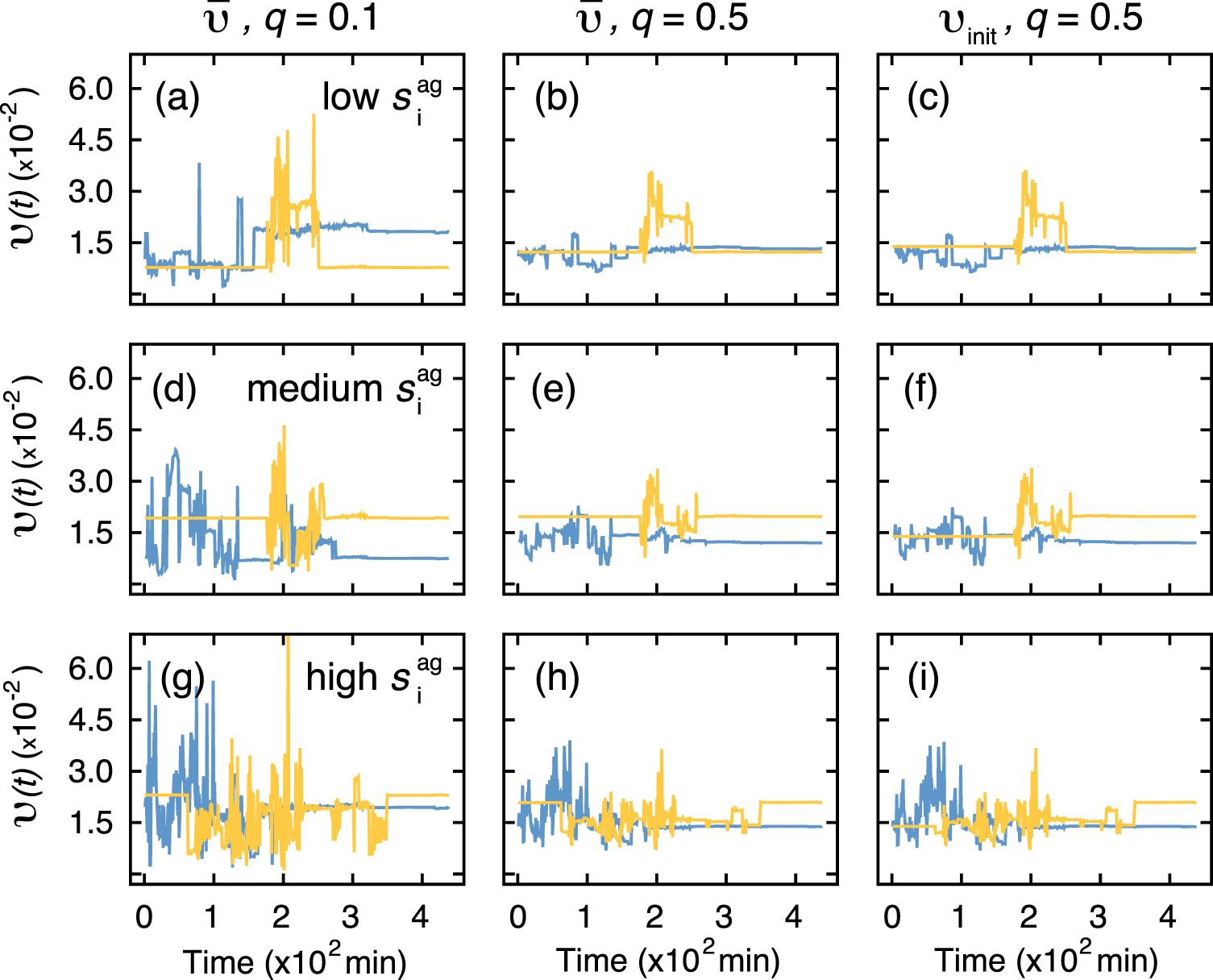
To examine this point, we measure the temporal fluctuation of the density of random walkers within a cycle. For the SPC data set, the stationary density at the tth snapshot, i.e. ${{v}_{i}}(t)$ , for six nodes is shown as a function of t in figures 3(a), (d), (g) with q = 0.1 and figures 3(b), (e), (h) with q = 0.5. Each panel represents the time course of the stationary density for two representative nodes i with low, intermediate and high strengths in the aggregate network, i.e. the total number of contacts, $s_{i}^{{\mbox{ag}}}$ . The corresponding results for the SPM data set are shown in figure 4. The results for the other data sets are shown in the appendix. Figures 3 and 4 indicate that the fluctuation of ${{v}_{i}}(t)$ is large irrespective of the strength of the node, although it is larger for nodes with larger strength values. The density of walkers remains constant at times when nodes are not making contacts. In particular, we identify plateaus for some ranges of t, which correspond to night periods in the case of the SPC network (figure 3) and the SPH network (see the appendix). In the SPM network (figure 4), most plateaus correspond to earlier or later times because visits are organized in groups in this museum, allowing interactions only within limited time windows. The fluctuations decrease as q increases. This behavior is expected because the stationary density approaches the uniform density as q increases.

**Figure 3.** Time dependence of the stationary density of the random walk for the SPC data set. In (a), (b), (d), (e), (g) and (h), the density of walkers ${\boldsymbol{v}} (t)={\boldsymbol{\bar{v}B}} (1)\cdots {\boldsymbol{B}} (t-1)$ is shown. In (c), (f) and (i), the density of walkers in a snapshot t calculated by ${\boldsymbol{v}} (t)={{{\boldsymbol{v}} }_{{\mbox{init}}}}(1){\boldsymbol{B}} (1)\cdots {\boldsymbol{B}} (t-1)$ , where ${{{\boldsymbol{v}} }_{{\mbox{init}}}}(1)=(1\ \cdots \ 1)/N$ , is shown. Each curve corresponds to a node with different $s_{i}^{{\mbox{ag}}}$ ; the two curves in each panel represent two representative nodes in the corresponding node-strength category. We set q = 0.1 in (a), (d), (g) and q = 0.5 in (b), (c), (e), (f), (h), (i). The resolution is ${{T}_{w}}=5$ min.
Download figure:
Standard image High-resolution image

**Figure 3.** Time dependence of the stationary density of the random walk for the SPC data set. In (a), (b), (d), (e), (g) and (h), the density of walkers ${\boldsymbol{v}} (t)={\boldsymbol{\bar{v}B}} (1)\cdots {\boldsymbol{B}} (t-1)$ is shown. In (c), (f) and (i), the density of walkers in a snapshot t calculated by ${\boldsymbol{v}} (t)={{{\boldsymbol{v}} }_{{\mbox{init}}}}(1){\boldsymbol{B}} (1)\cdots {\boldsymbol{B}} (t-1)$ , where ${{{\boldsymbol{v}} }_{{\mbox{init}}}}(1)=(1\ \cdots \ 1)/N$ , is shown. Each curve corresponds to a node with different $s_{i}^{{\mbox{ag}}}$ ; the two curves in each panel represent two representative nodes in the corresponding node-strength category. We set q = 0.1 in (a), (d), (g) and q = 0.5 in (b), (c), (e), (f), (h), (i). The resolution is ${{T}_{w}}=5$ min.
Download figure:
Standard image High-resolution image

**Figure 4.** Time dependence of the stationary density of the random walk for the SPM data set. The resolution is ${{T}_{w}}=1$ min. See the legend of figure 3 for other details.
Download figure:
Standard image High-resolution image

**Figure 4.** Time dependence of the stationary density of the random walk for the SPM data set. The resolution is ${{T}_{w}}=1$ min. See the legend of figure 3 for other details.
Download figure:
Standard image High-resolution image

Similar temporal fluctuations are observed when the temporal networks are coarse-grained (i.e. with a low resolution), as shown in figures 5 and 6 for the SPC and SPM data sets, respectively. The same is valid for the other data sets (see the appendix). Therefore, large fluctuations are a general phenomenon irrespective of the temporal resolution.

**Figure 5.** Time dependence of the stationary density for the SPC data set with a lower resolution. The resolution is ${{T}_{w}}=20$ min. See the legend of figure 3 for other details.
Download figure:
Standard image High-resolution image

**Figure 5.** Time dependence of the stationary density for the SPC data set with a lower resolution. The resolution is ${{T}_{w}}=20$ min. See the legend of figure 3 for other details.
Download figure:
Standard image High-resolution image

**Figure 6.** Time dependence of the stationary density for the SPM data set with a lower resolution. The resolution is ${{T}_{w}}=10$ min. See the legend of figure 3 for other details.
Download figure:
Standard image High-resolution image

**Figure 6.** Time dependence of the stationary density for the SPM data set with a lower resolution. The resolution is ${{T}_{w}}=10$ min. See the legend of figure 3 for other details.
Download figure:
Standard image High-resolution image

The large fluctuations revealed in figures 3–6 suggest that a node should be adjacent to nodes with high density of walkers at the right moment to secure a large ${{\bar{v}}_{i}}$ value, in favor of the right-moment principle. Nevertheless, the high accuracy of the in-strength approximation does not support the relevance of the right-moment principle.

We can resolve this apparent paradox as follows. The in-strength in the effective network, $s_{i}^{{\mbox{tp}}}(1)$ , consists of the contributions from different neighbors (i.e. jʼs in equation (20). Each $w_{ji}^{{\mbox{tp}}}(1)$ is equal to the number of temporal paths from j to i in the one cycle starting and ending at t = 1 and t = r, respectively. Each path is weighted by the out-degree of the source nodes on the path. If the out-degree of j is large at t = 1, the flow of the random walk is equally divided by the downstream neighbors such that a downstream neighbor of j, denoted by ${{k}_{1}}$ , receives a relatively small inflow of the random walk. Then, at t = 2, node ${{k}_{1}}$ , which has received the inflow of probability from its upstream neighbors (including j) at t = 1, sends the flow to ${{k}_{1}}$ ʼs downstream neighbors at t = 2. If the number of neighbors is large, then each downstream neighbor of ${{k}_{1}}$ at t = 2 receives a small inflow. Finally, $s_{i}^{{\mbox{tp}}}(1)$ is the total inflow, or weighted path count summed over all the starting nodes j at t = 1. The crucial observation here is that in the in-strength definition, the starting node is not weighted. In contrast, the exact calculation of ${{v}_{i}}(1)$ assumes that the starting node is weighted according to the stationary density ${{v}_{j}}(1)$ , as indicated in the first equality in equation (21).

Therefore, the fact that the in-strength approximation works well implies that the fluctuation of the density of walkers within a cycle starting from the uniform density and that starting from the stationary density do not significantly differ. This is in fact observed. In figures 3(c), 3(f), 3(i) 4(c), 4(f) and 4(i), we show the fluctuation of the density of walkers starting from the uniform density, i.e. $(1\ \cdots \ 1)/N$ for the same selected nodes as those in figures 3(b), 3(e), 3(h), 4(b), 4(e) and 4(h) (which correspond to the initial condition ${\boldsymbol{v}} (1)$ ). The fluctuation is similar between the two initial conditions except in early snapshots. Therefore, we conclude that the right-moment principle is logically present but practically unimportant.

4.5. Justification of periodic boundary conditions

We have assumed periodic boundary conditions to transform the original one-shot contact sequence into an infinitely repeated sequence. This is simply a technical solution to well define the stationary density. However, empirical networks have finite observation times and do not repeat themselves.

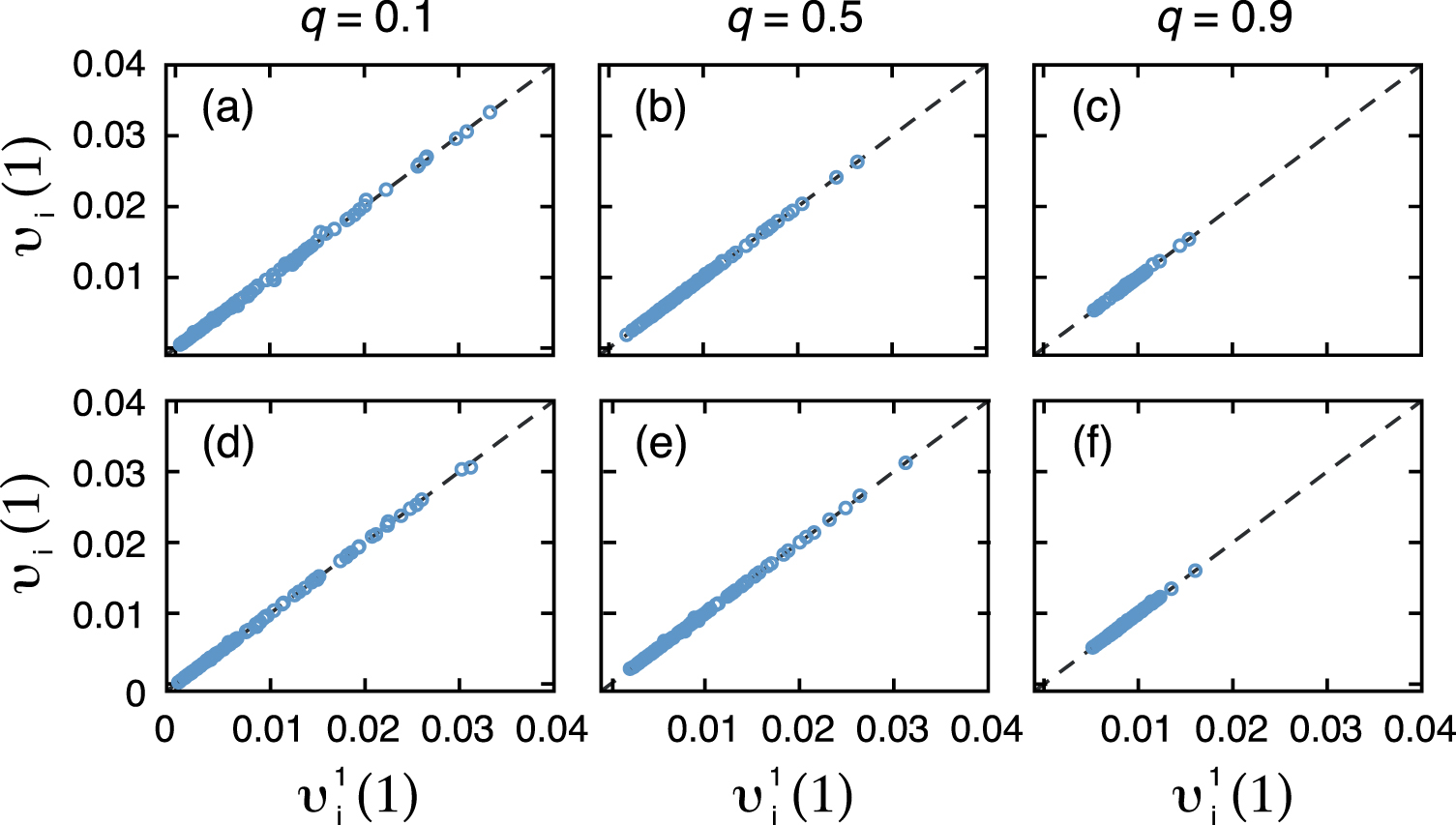
We justify the periodic boundary conditions, at least for sufficiently long data sets, because the repeated application of ${{{\boldsymbol{P}} }^{{\mbox{tp}}}}$ is practically unnecessary to approximate the stationary density. To show this point, we compare the stationary density and the density of walkers after a single application of ${{{\boldsymbol{P}} }^{{\mbox{tp}}}}$ . Note that the contact sequence is not repeated in the latter case. For various sojourn probabilities q, the two densities are shown for different nodes for the SPC (figure 7) and SPM (figure 8) data sets. The figures indicate that the density of walkers at most nodes after a single application of ${{{\boldsymbol{P}} }^{{\mbox{tp}}}}$ is sufficiently close to that in the stationary state. The result that the fluctuation of the density of walkers after a transient little differs between different initial conditions (figures 3(c), 3(f), 3(i) 4(c), 4(f) and 4(i)) is also consistent with the results shown in figures 7 and 8.

**Figure 7.** Density of walkers after a number of iterations of the power method for the SPC data set. $v_{i}^{1}$ (1) is the density of walkers after a single application of ${{{\boldsymbol{P}} }^{{\mbox{tp}}}}$ and ${{v}_{i}}(1)$ is the density of walkers in the stationary state. In (a)–(c) the resolution is ${{T}_{w}}=5$ min and in (d)–(f) the resolution is ${{T}_{w}}=10$ min. The initial conditions are given by the uniform distribution, i.e. ${{{\boldsymbol{v}} }_{{\mbox{init}}}}(1)=(1\ \cdots \ 1)/N$ .
Download figure:
Standard image High-resolution image

**Figure 7.** Density of walkers after a number of iterations of the power method for the SPC data set. $v_{i}^{1}$ (1) is the density of walkers after a single application of ${{{\boldsymbol{P}} }^{{\mbox{tp}}}}$ and ${{v}_{i}}(1)$ is the density of walkers in the stationary state. In (a)–(c) the resolution is ${{T}_{w}}=5$ min and in (d)–(f) the resolution is ${{T}_{w}}=10$ min. The initial conditions are given by the uniform distribution, i.e. ${{{\boldsymbol{v}} }_{{\mbox{init}}}}(1)=(1\ \cdots \ 1)/N$ .
Download figure:
Standard image High-resolution image

**Figure 8.** Density of walkers after a number of iterations of the power-method for the SPM data set. $v_{i}^{1}(1)$ is the density of walkers after a single application of P ^tp and ${{v}_{i}}(1)$ is the density of walkers in the stationary state. In (a)–(c) the resolution is ${{T}_{w}}=5$ min and in (d)–(f) the resolution is ${{T}_{w}}=10$ min. The initial conditions are given by the uniform distribution, i.e. ${{{\boldsymbol{v}} }_{{\mbox{init}}}}(1)=(1\ \cdots \ 1)/N$ .
Download figure:
Standard image High-resolution image

**Figure 8.** Density of walkers after a number of iterations of the power-method for the SPM data set. $v_{i}^{1}(1)$ is the density of walkers after a single application of P ^tp and ${{v}_{i}}(1)$ is the density of walkers in the stationary state. In (a)–(c) the resolution is ${{T}_{w}}=5$ min and in (d)–(f) the resolution is ${{T}_{w}}=10$ min. The initial conditions are given by the uniform distribution, i.e. ${{{\boldsymbol{v}} }_{{\mbox{init}}}}(1)=(1\ \cdots \ 1)/N$ .
Download figure:
Standard image High-resolution image

4.6. Sensitivity analysis

We do not expect that TempoRank is robust against variations in the temporal resolution ${{T}_{w}}$ , because changing ${{T}_{w}}$ alters the ordering of link activation and thus the potential paths selected by the walkers. The dependence of the TempoRank on ${{T}_{w}}$ is shown in figure 9 for three arbitrarily selected nodes. Both the TempoRank value and the rank based on it depend on ${{T}_{w}}$ . In particular, some nodes possess large TempoRank values in narrow ranges of ${{T}_{w}}$ . However, some other nodes have relatively stable TempoRank values.

**Figure 9.** Dependence of the TempoRank on the size of the time window, ${{T}_{w}}$ . TempoRank for three arbitrarily selected nodes for (a) SPC and (b) SPM data sets. We set q = 0.5.
Download figure:
Standard image High-resolution image

**Figure 9.** Dependence of the TempoRank on the size of the time window, ${{T}_{w}}$ . TempoRank for three arbitrarily selected nodes for (a) SPC and (b) SPM data sets. We set q = 0.5.
Download figure:
Standard image High-resolution image

A large value of the sojourn probability q slows down the walker so that the network changes faster than the walker explores the network. Then, the walker would not capture the temporal variations of the network. The dependence of the TempoRank on q is shown in figure 10 for five arbitrary nodes. As expected, the ranking as well as the values of the TempoRank depend on q. Note that all nodes have the same TempoRank values at q = 1.

**Figure 10.** Dependence of the TempoRank on the sojourn probability, q. TempoRank for arbitrarily selected five nodes for (a) SPC and (b) SPM data sets. We set ${{T}_{w}}=5$ min.
Download figure:
Standard image High-resolution image

**Figure 10.** Dependence of the TempoRank on the sojourn probability, q. TempoRank for arbitrarily selected five nodes for (a) SPC and (b) SPM data sets. We set ${{T}_{w}}=5$ min.
Download figure:
Standard image High-resolution image

5. Discussion

We proposed the TempoRank, a node centrality measure for temporal networks. In addition to the exact computation, we showed that the TempoRank is accurately approximated by the in-strength of the node in the effective network for some data sets of human interaction. The effective network is a directed network induced by the undirected temporal network. The concept of the effective network may be useful for other purposes, such as path counting of temporal networks and revealing information or viral flow along the arrow of time. A similar concept named exposure graph, used to define who can reach who in time, was previously exploited to study temporal centrality in the context of epidemic and information spread (see e.g. [46]).

In static directed networks, the stationary density of the random walk often deviates substantially from the in-degree [40, 47, 48], whereas it is accurate in other cases [37–41, 48]. We found that the in-strength of the effective network approximates the TempoRank, i.e. the stationary density in the effective (directed) network, with high accuracy. There are at least two possible reasons underlying the high accuracy of the in-strength approximation.

First, the effective network is usually dense. In general, if there is a directed temporal path from node i to node j in the given temporal network, $w_{ij}^{{\mbox{tp}}}> 0$ . Therefore, the link density in the effective network is equal to the so-called reachability measure [49], except for the difference in the treatment of the diagonal elements $w_{ii}^{{\mbox{tp}}}$ (1). In many temporal network data sets, the reachability is moderately or very large even if each snapshot in the temporal network is sparse [49–53] unless the number of snapshots (i.e. r) is too small. Then, the effective networks are dense. In this situation, the summation is taken over many upstream neighbors of node i for calculating ${{v}_{i}}(1)$ (first equality in equation (21)). Then, the heterogeneity in the TempoRank among the upstream neighbors of i, because of which the in-strength may deviate from ${{v}_{i}}(1)$ (equation (21)), may efficiently cancel out to yield similarity between the in-strength and ${{v}_{i}}(1)$ .

Second, the in-strength may be a significantly better approximator than the in-degree in general static and temporal networks. In the random walk on model temporal networks, the stationary density is only weakly correlated with the degree of the aggregate network [27]. Investigating the performance of the in-strength approximator in this situation and also on static networks may be an interesting research question.

We assumed the periodic boundary condition in time to define the stationary density of the random walk. In fact, a real temporal network data set does not repeat itself; the first snapshot does not follow the last snapshot. In addition, temporal network data are often non-stationary, swamped by frequent overturns of nodes and links even within a recording period [54–56]. A justification of the use of the periodic boundary condition is that the convergence of the power iteration seems to be very fast unless the number of snapshots is small. This was observed when we started from different initial conditions to have almost the same density of walkers at various nodes after a short transient within a single cycle (comparison between panels (b), (e), (h) and panels (c), (f), (i) in figures 3–6). The fast convergence was also supported by the fact that just a one-shot application of the transition matrix transforms a uniform initial density to an approximately stationary density. Therefore, the TempoRank represents the probability flow as we sequentially apply the snapshots in a single cycle at least for the data sets analyzed in the present study. Investigating the generalizability of this result warrants future work.

The diffusive dynamics in the continuous time is described by Laplacian dynamics. The Laplacian dynamics driven by the unnormalized Laplacian matrix has uniform stationary density both for the temporal network represented by a succession of snapshots and the aggregate network [57]. In contrast, we showed that the stationary density differed between the temporal and aggregate networks when the diffusive dynamics was considered in discrete time. A lesson drawn from this consideration is that we should be careful in discrete versus continuous time when considering diffusive processes on temporal networks. Analyzing a continuous-time counterpart of the TempoRank or the stationary density, as touched upon in [30, 31], requests further studies. The continuous-time random walk allows for independently controlling the speed of the walker and the aggregation window, which is useful for studying systems in which the diffusion may be faster or slower than the variations in the network structure. Nevertheless, if one uses the random walk to mimic real processes, the speed of the walker may be as difficult to estimate as the sojourn probability in the discrete-time formalism.

To assure the mixing property in arbitrary connected temporal networks, we assumed that the walker resided in the current node with probability q. The original PageRank employs the so-called teleportation probability to make the random walk mixing for arbitrary static networks [12, 13]. The sojourn probability q, however, is unrelated to the teleportation probability. The latter dictates that a walker jumps to an arbitrary node with a given equal probability irrespective of the current position, while q specifies the laziness of the random walk to move, as assumed in [34]. In our model, a random global jump probability is unnecessary because the initial network is assumed to be undirected and periodic boundary conditions are adopted, which removes the possibility that walkers are trapped on certain nodes. Furthermore, the teleportation adds another hyperparameter (i.e. the teleportation probability) and blurs the effect of the original network because it is a network-independent random jump. However, the teleportation would be necessary if we extend the present framework to the case of directed temporal networks.

Acknowledgements

We acknowledge Jean-Pierre Eckmann for kindly providing to us the data used in [23]. We thank Ryosuke Nishi and Taro Takaguchi for careful reading of the manuscript. LECR is a Chargé de recherches of the Fonds de la Recherche Scientifique — FNRS and thanks support from the Swedish Research Council (VR). NM acknowledges the support provided through Grants-in-Aid for Scientific Research (No. 23681033) from MEXT, Japan, the Nakajima Foundation and JSPS and FRS-FNRS under the Japan–Belgium Research Cooperative Program.

: Appendix

The appendix contains the results for the in-strength approximation and for the right-moment hypothesis for the SPH, SEX and EMA data sets. These results agree with the theoretical predictions described in the main text.

Appendix. In-strength approximation

The performance of the in-strength approximator for three values of the sojourn probability q is shown in figure A1 (SPH), figure A2 (SEX) and figure A3 (EMA). The in-strength approximation (panels (a)–(c)) is accurate for all tested values of q (i.e. from 0.1 to 0.9). As is the case for the other data sets, the in-strength of the aggregate network, i.e. $s_{i}^{{\mbox{ag}}}$ , which gives the exact stationary density of the random walk on the aggregate network, is little correlated with ${{v}_{i}}$ (1) for the same three values of q (panels (d)–(f)). The in-strength approximator for the TempoRank (see the main text) is also strongly correlated with ${{\bar{v}}_{i}}$ (panels (g)–(i)). Correlation is stronger for the SPH data set in comparison to SEX and EMA data sets which correspond to considerable sparser networks.

**Figure A1.** TempoRank for SPH network. (a)–(c) Relationship between the stationary density of the temporal transition matrix and the in-strength approximation. Each circle represents a node and the dashed lines represent the diagonal. (d)–(f) Relationship between the stationary density of the temporal transition matrix and the in-strength of the aggregate network. (g)–(i) Relationship between the TempoRank and the time-averaged in-strength of the effective network. We set q = 0.1 in (a), (d), (g), q = 0.5 in (b), (e), (h) and q = 0.9 in (c), (f), (i). The resolution is ${{T}_{w}}=5$ min.
Download figure:
Standard image High-resolution image

**Figure A2.** TempoRank for SEX network. The resolution is ${{T}_{w}}=2$ d. See the legends of figure A1 for other details. The axes are in log-scale.
Download figure:
Standard image High-resolution image

**Figure A2.** TempoRank for SEX network. The resolution is ${{T}_{w}}=2$ d. See the legends of figure A1 for other details. The axes are in log-scale.
Download figure:
Standard image High-resolution image

**Figure A3.** TempoRank for EMA network. The resolution is ${{T}_{w}}=1$ hour. See the legends of figure A1 for other details. The axes are in log-scale.
Download figure:
Standard image High-resolution image

**Figure A3.** TempoRank for EMA network. The resolution is ${{T}_{w}}=1$ hour. See the legends of figure A1 for other details. The axes are in log-scale.
Download figure:
Standard image High-resolution image

Appendix. The right-moment hypothesis

The stationary density at the tth snapshot, i.e ${\boldsymbol{v}} (t)$ , is shown as a function of t in figure A4 (SPH), figure A5 (SEX) and figure A6 (EMA). In each figure, we use two values of $q$ and calculate ${{v}_{i}}(t)$ for representative nodes i with low, intermediate and high strengths in the aggregate network, i.e. the total number of contacts, $s_{i}^{{\mbox{ag}}}$ . Fluctuations are significant in all cases.