


Abstract
Quantum phase estimation (QPE) is the workhorse behind any quantum algorithm and a promising method for determining ground state energies of strongly correlated quantum systems. Low-cost QPE techniques make use of circuits which only use a single ancilla qubit, requiring classical post-processing to extract eigenvalue details of the system. We investigate choices for phase estimation for a unitary matrix with low-depth noise-free or noisy circuits, varying both the phase estimation circuits themselves as well as the classical post-processing to determine the eigenvalue phases. We work in the scenario when the input state is not an eigenstate of the unitary matrix. We develop a new post-processing technique to extract eigenvalues from phase estimation data based on a classical time-series (or frequency) analysis and contrast this to an analysis via Bayesian methods. We calculate the variance in estimating single eigenvalues via the time-series analysis analytically, finding that it scales to first order in the number of experiments performed, and to first or second order (depending on the experiment design) in the circuit depth. Numerical simulations confirm this scaling for both estimators. We attempt to compensate for the noise with both classical post-processing techniques, finding good results in the presence of depolarizing noise, but smaller improvements in 9-qubit circuit-level simulations of superconducting qubits aimed at resolving the electronic ground state of a H4-molecule.
Export citation and abstract BibTeX RIS

Original content from this work may be used under the terms of the Creative Commons Attribution 3.0 licence. Any further distribution of this work must maintain attribution to the author(s) and the title of the work, journal citation and DOI.
1. Introduction
It is known that any problem efficiently solvable on a quantum computer can be formulated as eigenvalue sampling of a Hamiltonian or eigenvalue sampling of a sparse unitary matrix [1]. In this sense the algorithm of quantum phase estimation (QPE) is the only quantum algorithm which can give rise to solving problems with an exponential quantum speed-up. Despite it being such a central component of many quantum algorithms, very little work has been done so far to understand what QPE in the current noisy intermediate scale quantum (NISQ) era of quantum computing [2] where quantum devices are strongly coherence-limited. QPE comes in many variants, but a large subclass of these algorithms (e.g. the semi-classical version of textbook phase estimation [3, 4], Kitaev's phase estimation [5], Heisenberg-optimized versions [6]), are executed in an iterative sequential form using controlled-Uk gates with a single ancilla qubit [7, 8] (see figure 1), or by direct measurement of the system register itself [6]. Such circuits are of practical interest in the near term when every additional qubit requires a larger chip and brings in additional experimental complexity and incoherence.

Figure 1. Circuit for the QPE experiments described in this work. The state  is defined in equation (3). The probability for the ancilla qubit to return the vector m of results in the absence of error is given by equation (10). The single-qubit rotation equals
  while H is the Hadamard gate.
Download figure:
Standard image High-resolution imageSome of the current literature on QPE works under limiting assumptions. The first is that one does not start in an eigenstate of the Hamiltonian [9, 10]. A second limitation is that one does not take into account the (high) temporal cost of running Uk [8] for large k when optimizing phase estimation. The size and shallowness of the QPE circuit is important since, in the absence of error correction or error mitigation, one expects entropy build-up during computation. This means that circuits with large k may not be of any practical interest.
The scenario where the input state is not an eigenstate of the unitary matrix used in phase estimation is the most interesting one from the perspective of applications, and we will consider it in this work. Such an input state can be gradually projected onto an eigenstate by the phase estimation algorithm and the corresponding eigenvalue can be inferred. However, for coherence-limited low-depth circuits one may not be able to evolve sufficiently long to project well onto one of the eigenstates. This poses the question what one can still learn about eigenvalues using low-depth circuits. An important point is that it is experimentally feasible to repeat many relatively shallow experiments (or perform them in parallel on different machines). Hence we ask what the spectral-resolving power of such phase estimation circuits is, both in terms of the number of applications of the controlled-U circuit in a single experiment, and the number of times the experiment is repeated. Such repeated phase estimation experiments require classical post-processing of measurement outcomes, and we study two such algorithms for doing this. One is our adaptation of the Bayesian estimator of [10] to the multiple-eigenvalue scenario. A second is a new estimator based on a treatment of the observed measurements as a time-series, and construction of the resultant time-shift operator. This latter method is very natural for phase estimation, as one interprets the goal of phase estimation as the reconstruction of frequencies present in the output of a temporal sound signal. In fact, the time-series analysis that we develop is directly related to what are called Prony-like methods in the signal-processing literature, see e.g. [11]. The use of this classical method in quantum signal processing, including in quantum tomography [12], seems to hold great promise.
One can interpret our results as presenting a new hybrid classical-quantum algorithm for QPE. Namely, when the number of eigenstates in an input state is small, i.e. scaling polynomially with the number of qubits  , the use of our classical post-processing method shows that there is no need to run a quantum algorithm which projects onto an eigenstate to learn the eigenvalues. We show that one can extract these eigenvalues efficiently by classically post-processing the data from experiments using a single-round QPE circuits (see section 2) and classically handling
  matrices. This constitutes a saving in the required depth of the quantum circuits.
The spectral-resolution power of QPE can be defined by its scaling with parameters of the experiment and the studied system. We are able to derive analytic scaling laws for the problem of estimating single eigenvalues with the time-series estimator. We find these to agree with the numerically-observed scaling of both studied estimators. For the more general situation, with multiple eigenvalues and experimental error, we study the error in estimating the lowest eigenvalue numerically. This is assisted by the low classical computation cost of both estimators. We observe scaling laws for this error in terms of the overlap between the ground and starting state (i.e. the input state of the circuit), the gap between the ground and excited states, and the coherence length of the system. In the presence of experimental noise we attempt to adjust our estimators to mitigate the induced estimation error. For depolarizing-type noise we find such compensation easy to come by, whilst for a realistic circuit-level simulation we find smaller improvements using similar techniques.
Even though our paper focuses on QPE where the phases corresponds to eigenvalues of a unitary matrix, our post-processing techniques may also be applicable to multi-parameter estimation problems in quantum optical settings. In these settings the focus is on determining an optical phase-shift [13–15] through an interferometric set-up. There is experimental work on (silicon) quantum photonic processors [16–18] on multiple-eigenvalue estimation for Hamiltonians which could also benefit from using the classical post-processing techniques that we develop in this paper.
2. Quantum phase estimation
QPE covers a family of quantum algorithms which measure a system register of  qubits in the eigenbasis of a unitary operator U [5, 19]

to estimate one or many phases ϕj. QPE algorithms assume access to a noise free quantum circuit which implements U on our system register conditioned on the state of an ancilla qubit. Explicitly, we require the ability to implement

where  and
and  are the computational basis states of the ancilla qubit, and
  is the identity operator on the system register.
In many problems in condensed matter physics, materials science, or computational chemistry, the object of interest is the estimation of spectral properties or the lowest eigenvalue of a Hamiltonian  . The eigenvalue estimation problem for
  can be mapped to phase estimation for a unitary
  with a τ chosen such that the relevant part of the eigenvalue spectrum induces phases within [−π, π). Much work has been devoted to determining the most efficient implementation of the (controlled)-
 operation, using exact or approximate methods [19–22]. Alternatively, one may simulate
  via a quantum walk, mapping the problem to phase estimating the unitary
  for some λ, which may be implemented exactly [23–26]. In this work we do not consider such variations, but rather focus on the error in estimating the eigenvalue phases of the unitary U that is actually implemented on the quantum computer. In particular, we focus on the problem of determining the value of a single phase ϕ0 to high precision (this phase could correspond, for example, to the ground state energy of some Hamiltonian
  ).
).
Phase estimation requires the ability to prepare an input, or starting state

with good overlap with the ground state; A0 ≫ 0. Note here that the spectrum of U may have exact degeneracies (e.g. those enforced by symmetry) which phase estimation does not distinguish; we count degenerate eigenvalues as a single ϕj throughout this work. The ability to start QPE in a state which already has good overlap with the ground state is a non-trivial requirement for the applicability of the QPE algorithm. On the other hand, it is a well-known necessity given the QMA-completeness [27] of the lowest eigenvalue problem5 . For many quantum chemistry and materials science problems it is known or expected that the Hartree–Fock state has good overlap with the ground state, although rigorous results beyond perturbation theory are far and few between (see e.g. [28]). Beyond this, either adiabatic evolution [20, 29] or variational quantum eigensolvers [30] can provide an approximate starting state to improve on via phase estimation.
Phase estimation is not limited to simply learning the value of ϕ0; it may obtain information about all phases ϕj as long as Aj > 0. However, the resources required to estimate  are bounded below by 1/Aj. To see this, note that the controlled-unitary
  does not mix eigenstates, and so there is no difference (in the absence of error) between starting with
  and the mixed state

The latter is then equivalent to preparing the pure state  with probability Aj, so if N preparations of
  are required to estimate ϕj to an error
  , the same error margin requires at least N/Aj preparations of the state
  . As the number of eigenstates
  with non-zero contribution to
  generally scales exponentially with the system size
  , estimating more than the first few ϕj (ordered by the magnitude Aj) will be unfeasible.
Low-cost (in terms of number of qubits) QPE may be performed by entangling the system register with a single ancilla qubit [5, 8, 10, 27]. In figure 1, we give the general form of the quantum circuit to be used throughout this paper. An experiment, labeled by a number n = 1, ..., N, can be split into one or multiple rounds r = 1, ..., Rn, following the preparation of the starting state  . In each round a single ancilla qubit prepared in the
  state controls
  where the integer kr can vary per round. The ancilla qubit is then rotated by
  (with the phase βr possibly depending on other rounds in the same experiment) and read out in the X-basis, returning a measurement outcome mr ∈ {0, 1}. We denote the chosen strings of integers and phases of a single multi-round experiment by k and
  , respectively. We denote the number of controlled-U iterations per experiment as
  . We denote the total number of controlled-U iterations over all experiments as

As the system register is held in memory during the entire time of the experiment, the choice of K is dictated by the coherence time of the underlying quantum hardware. Hence, we introduce a dimensionless coherence length

Here TU is the time required to implement a single application of controlled-U in equation (7), and Terr is the time-to-error of a single qubit, so that  is the time-to-failure of
  qubits. The idea is that Kerr bounds the maximal number of applications of U in an experiment, namely K ≤ Kerr.
A new experiment starts with the same starting state  . Values of kr and βr may be chosen independently for separate experiments n, i.e. we drop the label n for convenience. We further drop the subscript r from single-round experiments (with R = 1).
In the absence of error, one may calculate the action of the QPE circuit on the starting state (defined in equation (3)). Working in the eigenbasis of U on the system register, and the computational basis on the ancilla qubit, we calculate the state following the controlled-rotation  , and the rotation
  on the ancilla qubit to be

The probability to measure the ancilla qubit in the X-basis as m1 ∈ {0, 1} is then

and the unnormalized post-selected state of the system register is

The above procedure may then be repeated for r rounds to obtain the probability of a string  of measurement outcomes of one experiment as

Here,  is the vector of phases ϕj and
  the vector of probabilities for different eigenstates. We note that
  is independent of the order in which the rounds occur in the experiment. Furthermore, when
  ,
,  is equal to the product of the single-round probabilities
  , as there is no difference between a multi-round experiment and the same rounds repeated across individual experiments.
One can make a direct connection with parameter estimation work by considering the single-round experiment scenario in figure 1. The Hadamard gate putting the ancilla qubit in  and measuring the qubit in the X-basis are, in the optical setting, realized by beam-splitters, so that only the path denoted by the state
  will pick up an unknown phase-shift. When the induced phase-shift is not unique but depends, say, on the state of another quantum system, we may like to estimate all such possible phases corresponding to our scenario of wishing to estimate multiple eigenvalues. Another physical example is a dispersively coupled qubit-cavity mode system where the cavity mode occupation number will determine the phase accumulation of the coupled qubit [31].
3. Classical data analysis
Two challenges are present in determining ϕ0 from QPE experiments. First, we only ever have inexact sampling knowledge of  . That is, repeated experiments at fixed
  do not directly determine
  , but rather sample from the multinomial distribution
  . From the measurement outcomes we can try to estimate
  (and from this ϕ0) as a hidden variable. Secondly, when
  determining ϕ0 from
  poses a non-trivial problem.
Let us first consider the case  . Let us assume that we do single-round experiments with a fixed k for each experiment. Naturally, taking k = 1 would give rise to the lowest-depth experiments. If we start these experiments with k = 1 in the eigenstate
  , then one can easily prove that taking β = 0 or
  for half of the experiments, suffices to estimate ϕ0 with variance scaling as
  . This result can be derived using standard Chernoff bounds, see e.g. [32, 33], and represent standard sampling or shot noise behavior. When
  , N K-round experiments each with k = 1 are indistinguishable from N × K single-round experiments with k = 1. This implies that the same scaling holds for such multi-round experiments, i.e. the variance scales as
  .
.
Once the phase ϕ0 is known to sufficient accuracy, performing QPE experiments with k > 1 is instrumental in resolving ϕ0 in more detail, since the probability of a single-round outcome depends on kϕ0 [6]. Once one knows with sufficient certainty that  (for integer m), one can achieve variance scaling as
  (conforming to so-called local estimation Cramer–Rao bounds suggested in [10, 34]). A method achieving Heisenberg scaling, where the variance scales as
  (see equation (5)), was analyzed in [6, 32]. This QPE method can also be compared with the information-theoretic optimal maximum-likelihood phase estimation method of [8] where
  experiments are performed, each choosing a random
  to resolve ϕ0 with error scaling as 1/K. The upshot of these previous results is that, while the variance scaling in terms of the total number of unitaries goes like 1/Ktot when using k = 1, clever usage of k > 1 data can lead to
  scaling. However, as K is limited by Kerr in near-term experiments, this optimal Heisenberg scaling may not be accessible.
When  , the above challenge is complicated by the need to resolve the phase ϕ0 from the other ϕj. This is analogous to the problem of resolving a single note from a chord. Repeated single-round experiments at fixed k and varying β can only give information about the value of the function:

at this fixed k, since

This implies that information from single-round experiments at fixed k is insufficient to resolve ϕ0 when  , as g(k) is then not an invertible function of ϕ0 (try to recover a frequency from a sound signal at a single point in time!). In general, for multi-round experiments using a maximum of K total applications of
  , we may only ever recover g(k) for k ≤ K. This can be seen from expanding
  as a sum of
  terms with m + n ≤ K, which are in turn linear combinations of g(k) for k ≤ K. As we will show explicitly in the next section 3.1 this allows us to recover up to K ϕj. However, when
  , these arguments imply that we cannot recover any phases exactly. In this case, the accuracy to which we can estimate our target ϕ0 is determined by the magnitude of the amplitude A0 in the inital state
  as well as the gap towards the other eigenvalues. For example, in the limit
  , an unbiased estimation of ϕ0 using data from k = 1 would be

and the error in such estimation is

with our bound being independent of  . We are unable to extend this analysis beyond the k = 1 scenario, and instead we study the scaling in this estimation numerically in section 4. In the remainder of this section, we present two estimators for multi-round QPE. The first is an estimator based on a time-series analysis of the function g(k) using Prony-like [11] methods that has a low computation overhead. The second is a Bayesian estimator similar to that of [10], but adapted for multiple eigenphases ϕj.
3.1. Time-series analysis
Let us assume that the function g(k) in equation (11) is a well-estimated function at all points 0 ≤ k ≤ K, since the number of experiments N is sufficiently large. We may extend this function to all points  using the identity
  to obtain a longer signal6
. We wish to determine the dominant frequencies ϕj in the signal g(k) as a function of 'time' k. This can be done by constructing and diagonalizing a time-shift matrix
to obtain a longer signal6
. We wish to determine the dominant frequencies ϕj in the signal g(k) as a function of 'time' k. This can be done by constructing and diagonalizing a time-shift matrix  whose eigenvalues are the relevant frequencies in the signal, as follows.
We first demonstrate the existence of the time-shift matrix  in the presence of
  separate frequencies. Since we may not know
  , let us first estimate it as l. We then define the vectors
  ,
,  . These vectors can be decomposed in terms of single-frequency vectors

We can make a  matrix B with the components bj as columns

When  , the columns of B are typically linearly independent7
, hence the non-square matrix B is invertible and has a (left)-pseudoinverse B−1 such that B−1B = 1. Note however, when
, the columns of B are typically linearly independent7
, hence the non-square matrix B is invertible and has a (left)-pseudoinverse B−1 such that B−1B = 1. Note however, when  the columns of B are linearly-dependent, so B cannot be inverted. If B is invertible, we can construct the shift matrix
  with
with  . By construction,
  (as
(as  ), and thus

This implies that  acts as the time-shift operator mapping g(k) to g(k + 1). As the eigenvalues of
  are precisely the required phases
  in case
  , constructing and diagonalizing
  will obtain our desired phases including ϕ0. When
  , the eigen-equation for
  cannot have the solution bj since these are not linearly independent.
The above proof of existence does not give a method of constructing the time-shift operator  , as we do not have access to the matrices B or D. To construct
  from the data that we do have access to, we construct the
  Hankel matrices G(0), G(1) by

indexing 0 ≤ i ≤ l − 1,  . The kth column of G(a) is the vector
  , and so
  . We can thus attempt to find
  as a solution of the (least-squares) problem of minimizing
  . The rank of the obtained
  is bounded by the rank of G(0). We have that
  is at most
  since it is a sum over rank-1 matrices. At the same time
  . This implies that we require both
  and
and  to obtain a shift matrix
  with
with  eigenvalues. This is only possible when
  , giving an upper bound for the number of frequencies obtainable. When G(0) is not full rank (because
  ), this problem may have multiple zeros
  . However, when
  each of these must satisfy
  for
for  .
.
Then, as long as  , equation (14) is invertible by an operator C

It follows that

and then

so every  obtained in this way must have eigenvalues
  .
.
The above analysis is completely independent of the coefficients Aj. However, once the eigenvalues ϕj are known, the matrix B (equation (15)) may be constructed, and the Aj may be recovered by a subsequent least-squares minimization of

This allows us to identify spurious eigenvalues if  (as these will have a corresponding zero amplitude). Numerically, we find no disadvantage to then choosing the largest l permitted by our data, namely l = K.
Assuming a sufficient number of repetitions N these arguments imply that this strategy requires that  to determine all eigenvalues accurately. However, when
  there still exists a least-squares solution
  that minimizes
  . When A0 ≫ 1/K, we expect that
  should have eigenvalues
  that we can take as the estimator for ϕ0; the same is true for any other ϕj with sufficiently large Aj. In figure 2 we show an example of convergence of this estimation for multiple eigenvalues
  as
as  in the case where g(k) is known precisely (i.e. in the absence of sampling noise). The error
  when
when  depends on the eigenvalue gap above ϕ0, as well as the relative weights Aj, as we will see in section 4.3.

Figure 2. Convergence of the time-series estimator in the estimation of  eigenvalues (chosen at random with equally sized amplitudes Aj = 1/10) when the exact function g(k) is known at points 0, ..., K. The estimator constructs and calculates the eigenvalues of the K × K time-shift matrix
  which are shown as the red plusses in the figure. When
  (gray dashed line), the frequencies are attained to within machine precision. When
  , it is clear from the figure that the found eigenvalues provide some form of binning approximation of the spectrum.
Download figure:
Standard image High-resolution imageIn appendix B we derive what variance can be obtained with this time-series method in the case  , using single-round circuits with k = 1 up to K. Our analysis leads to the following scaling in N and K:

We will compare these results to numerical simulations in section 4.1.
3.1.1. Estimating g(k)
The function g(k) cannot be estimated directly from experiments, but may instead be created as a linear combination of  for different values of k and β. For single-round experiments, this combination is simple to construct:

For multi-round experiments, the combination is more complicated. In general,  is a linear combination of real and imaginary parts of g(l) with
  . This combination may be constructed by writing
  and
and  in terms of exponentials, and expanding. However, inverting this linear equation is a difficult task and subject to numerical imprecision. For some fixed choices of experiments, it is possible to provide an explicit expansion. Here we focus on K-round k = 1 experiments with K/2 β = 0 and K/2
  final rotations during each experiment (choosing K even). The formula for
  is independent of the order in which these rounds occur. Let us write
  as the probability of seeing both
  outcomes with mr = 1 in the K/2 rounds with βr = 0 and
  outcomes with nr = 1 in the K/2 rounds with βr = π/2. In other words,
  ,
,  are the Hamming weights of the measurement vectors split into the two types of rounds described above. Then, one can prove that, for 0 ≤ k ≤ K/2:

where

The proof of this equality can be found in appendix A.
Calculating g(k) from multi-round (k = 1) experiments contains an additional cost: combinatorial factors in equation (24) relate the variance in g(k) to the variance in  but the combinatorial pre-factor
  can increase exponentially in k. This can be accounted for by replacing the least squares fit used above with a weighted least squares fit, so that one effectively relies less on the correctness of g(k) for large k. To do this, we construct the matrix
  row-wise from the rows
  of G(1). That is, for the ith row
  we minimize

This equation may be weighted by multiplying G(0) and  by the weight matrix

where  is the standard deviation in our estimate of
  . Note that the method of weighted least-squares is only designed to account for error in the independent variable of a least squares fit, in our case this is G(1). This enhanced effect of the sampling error makes the time-series analysis unstable for large K. We can analyze how this weighting alters the previous variance analysis when
  . If we take this into account (see derivation in appendix B), we find that

for a time-series analysis applied to multi-round k = 1 experiments.
3.1.2. Classical computation cost
In practice, the time-series analysis can be split into three calculations; (1) estimation of  or
or  , (2) calculation of g(k) from these probabilities via equation (23) or equation (24), and (3) estimation of the phases ϕ from g(k). Clearly (2) and (3) only need to be done once for the entire set of experiments.
The estimation of the phases ϕ requires solving two least squares equations, with cost  (recalling that l is the number of frequencies to estimate, and K is the maximum known value of g(k)), and diagonalizing the time-shift matrix
  with cost O(l3). For single-round phase estimation this is the dominant calculation, as calculating g(k) from equation (23) requires simply K additions. As a result this estimator proves to be incredibly fast, able to estimate one frequency from a set of N = 106 experiments of up to K = 10 000 in <100 ms, and l = 1000 frequencies from N = 106 experiments with K = 1000 in <1 min. However, for multi-round phase estimation the calculation of g(k) in equation (24) scales as O(K4). This then dominates the calculation, requiring 30 s to calculate 50 points of g(k). (All calculations performed on a 2.4 GHz Intel i3 processor.) We note that all the above times are small fractions of the time required to generate the experimental data when N ≫ K, making this a very practical estimator for near-term experiments.
3.2. Efficient Bayesian analysis
When the starting state is the eigenstate  , the problem of determining ϕ0 based on the obtained multi-experiment data has a natural solution via Bayesian methods [10, 35]. Here we extend such Bayesian methodology to a general starting state. For computational efficiency we store a probability distribution over phases P(ϕ) using a Fourier representation of this periodic function P(ϕ) (see appendix C). This technique can also readily be applied to the case of Bayesian phase estimation applied to a single eigenstate.
A clearly information-theoretic optimal Bayesian strategy is to choose the  and
and  based on the data obtained in some N experiments [8]. After these N experiments, leading to qubit measurement outcomes
  , one can simply choose
  which maximizes the posterior distribution:

In other words, one chooses

A possible way of implementing this strategy is to (1) assume the prior distribution to be independent of A and  and (2) estimate the maximum by assuming that the derivative with respect to A and
  vanishes at this maximum.
Instead of this method we update our probability distribution over  and A after each experiment. After experiment n the posterior distribution
  via Bayes' rule reads

To calculate the updates we will assume that the distribution over the phases ϕj and probabilities Aj are independent, that is

As prior distribution we take  with a flat prior
  , given the absence of a more informed choice. We take
  , with A0 and Σ2 approximate mean and covariance matrices. We need to do this to break the symmetry of the problem, so that
  is estimating ϕ0 and not any of the other ϕs. We numerically find that the estimator convergence is relatively independent of our choice of A0 and Σ2.
The approximation in equation (31) allows for relatively fast calculations of the Bayesian update of  , and an approximation to the maximum-likelihood estimation of
  . Details of this computational implementation are given in (C1).
3.2.1. Classical computation cost
In contrast to the time-series estimator, the Bayesian estimator incurs a computational cost in processing the data from each individual experiment. On the other hand, obtaining the estimate  for ϕ0 is simple, once one has the probability distribution
  :
:

A key parameter here is the number of frequencies #freq stored in the Fourier representation of P(ϕ); each update requires multiplying a vector of length  by a sparse matrix. Our approximation scheme for calculating the update to A makes this multiplication the dominant time cost of the estimation. As we argue in (C1) one requires
  to store a fully accurate representation of the probability vector. For the single-round scenario with kr = 1, hence Ktot = N, we find a large truncation error when #freq ≪ N, and so the computation cost scales as N2. In practice we find that processing the data from N < 104 experiments takes seconds on a classical computer, but processing more than 105 experiments becomes rapidly unfeasible.
3.3. Experiment design
Based on the considerations above we seek to compare some choices for the meta-parameters in each experiment, namely the number of rounds, and the input parameters kr and βr for each round.
Previous work [10, 36], which took as a starting state the eigenstate  , formulated a choice of k and β, using single-round experiments and Bayesian processing, namely

Roughly, this heuristic adapts to the expected noise in the circuit by not using any k such that the implementation of Uk takes longer than  . It also adapts k to the standard-deviation of the current posterior probability distribution over
  : a small standard-deviation after the nth experiment implies that k should be chosen large to resolve the remaining bits in the binary expansion of ϕ08
.
: a small standard-deviation after the nth experiment implies that k should be chosen large to resolve the remaining bits in the binary expansion of ϕ08
.
In this work we use a starting state which is not an eigenstate, and as such we must adjust the choice in equation (32). As noted in section 3, to separate different frequency contributions to g(k) we need good accuracy beyond that at a single value of k. The optimal choice of the number of frequencies to estimate depends on the distribution of the Aj, which may not be well known in advance. Following the inspiration of [10], we choose for the Bayesian estimator

We thus similarly bound K depending how well one has already converged to a value for ϕ0 which constitutes some saving of resources. At large N we numerically find little difference between choosing k at random from {1, ..., K} and cycling through k = 1, ..., K in order. For this Bayesian estimator we draw β at random from a uniform distribution [0, 2π). We find that the choice of β has no effect on the final estimation (as long as it is not chosen to be a single number) For the time-series estimator applied to single-round experiments, we choose to cycle over k = 1, ..., K so that it obtains a complete estimate of g(k) as soon as possible, taking an equal number of experiments with final rotation β = 0 and β = π/2 at each k. Here again K ≤ Kerr, so that we choose the same number of experiments for each k ≤ K. For the time-series estimator applied to multi-round experiments, we choose an equal number of rounds with β = 0 and β = π/2, taking the total number of rounds equal to R = K.
4. Results without experimental noise
We first focus on the performance of our estimators in the absence of experimental noise, to compare their relative performance and check the analytic predictions in section 3.1. Although with a noiseless experiment our limit for K is technically infinite, we limit it to a make connection with the noisy results of the following section. Throughout this section we generate results directly by calculating the function  and sampling from it. Note that
  only depends on
  and not on the number of qubits in the system.
4.1. Single eigenvalues
To confirm that our estimators achieve the scaling bounds discussed previously, we first test them on the single eigenvalue scenario  . In figure 3, we plot the scaling of the average absolute error in an estimation
  of a single eigenvalue ϕ ∈ [−π, π), defined so as to respect the 2π-periodicity of the phase:

as a function of varying N and K. Here  represents an average over repeated QPE simulations, and the Arg function is defined using the range [−π, π) (otherwise the equality does not hold).

Figure 3. Estimator performance for single eigenvalues with single and multi-round k = 1 QPE schemes. Plots show scaling of the mean absolute error (equation (35)) with (top) the number of experiments (at fixed K = 50), with (middle) K for a fixed total number of experiments (N = 106), and (bottom) with K with a fixed number (100) of experiments per k = 1, ..., K (i.e.  ). Data is averaged over 200–500 QPE simulations, with a new eigenvalue chosen for each simulation. Shaded regions (top) and error bars (middle, bottom) give 95% confidence intervals. Dashed lines show the scaling laws of equation (22) (fitted by eye). The top-right legend labeling the different estimation schemes is valid for all three plots.
Download figure:
Standard image High-resolution imageWe see that both estimators achieve the previously-derived bounds in 3.1 (overlayed as dashed lines), and both estimators achieve almost identical convergence rates. The results for the Bayesian estimation match the scaling observed in [10]. Due to the worse scaling in K, the multi-round k = 1 estimation significantly underperforms single-round phase estimation. This is a key observation of this paper, showing that if the goal is to estimate a phase rather than to project onto an eigenstate, it is preferable to do single-round experiments.
4.2. Example behavior with multiple eigenvalues
The performance of QPE is dependent on both the estimation technique and the system being estimated. Before studying the system dependence, we first demonstrate that our estimators continue to perform at all in the presence of multiple eigenvalues. In figure 4, we demonstrate the convergence of both the Bayesian and time-series estimators in the estimation of a single eigenvalue ϕ0 = −0.5 of a fixed unitary U, given a starting state  which is a linear combination of 10 eigenstates
  . We fix
  , and draw other eigenvalues and amplitudes at random from [0, π] (making the minimium gap ϕj − ϕ0 equal to 0.5). We perform 2000 QPE simulations with K = 50, and calculate the mean absolute error (equation (35), solid), Holevo variance
  (dashed), and root mean squared error
  (dotted), given by

We observe that both estimators retain their expected  , with one important exception. The Bayesian estimator occasionally (10% of simulations) estimates multiple eigenvalues near ϕ0. When this occurs, the estimations tend to repulse each other, making neither a good estimation of the target. This is easily diagnosable without knowledge of the true value of ϕ0 by inspecting the gap between estimated eigenvalues. While using this data to improve estimation is a clear target for future research, for now we have opted to reject simulations where such clustering occurs (in particular, we have rejected data points where
  ). That this is required is entirely system-dependent: we find the physical Hamiltonians studied later in this text to not experience this effect. We attribute this difference to the distribution of the amplitudes Aj—physical Hamiltonians tend to have a few large Aj, whilst in this simulation the Aj were distributed uniformly.

Figure 4. Scaling of error for time-series (dark green) and Bayesian (red) estimators with the number of experiments performed for a single shot of a unitary with randomly drawn eigenphases (parameters given in text). Three error metrics are used as marked (described in text—note that the mean squared error and Holevo variance completely overlap for the time-series estimator). Data is averaged over 2000 simulations. The peak near N = 3000 comes from deviation in a single simulation and is not of particular interest. With this exception, error bars are approximately equal to width of the lines used. (Inset) histogram of the estimated phases after N = 104 experiments. Blue bars correspond to Bayesian estimates that were rejected (rejection method described in text). These have been magnified 10× to be made visible.
Download figure:
Standard image High-resolution imageIn the inset to figure 4, we plot a histogram of the estimated eigenphases after N = 104 experiments. For the Bayesian estimator, we show both the selected (green) and rejected (blue) eigenphases. We see that regardless of whether rejection is used, the distribution appears symmetric about the target phase ϕ0. This suggests that in the absence of experimental noise, both estimators are unbiased. Proving this definitively for any class of systems is difficult, but we expect both estimators to be unbiased provided A0 ≫ 1/K. When A0 ≤ 1/K, one can easily construct systems for which no phase estimation can provide an unbiased estimation of ϕ0 (following the arguments of section 3). We further see that the scaling of the rms error rms and the Holevo variance match the behavior of the mean absolute error , implying that our results are not biased by the choice of estimator used.
4.3. Estimator scaling with two eigenvalues
The ability of QPE to resolve separate eigenvalues at small K can be tested in a simple scenario of two eigenvalues, ϕ0 and ϕ1. The input to the QPE procedure is then entirely characterized by the overlap A0 with the target state  , and the gap
  .
.
In figure 5, we study the performance of our time-series estimator in estimating ϕ0 after N = 106 experiments with K = 50, measured again by the mean error (equation (35)). We show a two-dimensional plot (averaged over 500 simulations at each point A0, δ) and log–log plots of one-dimensional vertical (lower left) and horizontal (lower right) cuts through this surface. Due to computational costs, we are unable to perform this analysis with the Bayesian estimator, or for the multi-round scenario. We expect the Bayesian estimator to have similar performance to the time-series estimator (given their close comparison in sections 4.1 and 4.2). We also expect the error in multi-round QPE to follow similar scaling laws in A0 and δ as single-round QPE (i.e. multi-round QPE should be suboptimal only in its scaling in K).

Figure 5. Performance of the time-series estimator in the presence of two eigenvalues. (Top) surface plot of the error after N = 106 experiments for K = 50, as a function of the overlap A0 with the target state  , and the gap
  . Plot is divided by hand into three labeled regions where different scaling laws are observed. Each point is averaged over 500 QPE simulations. (bottom) log–log plots of vertical (bottom left) and horizontal (bottom right) cuts through the surface, at the labeled positions. Dashed lines in both plots are fits (by eye) to the observed scaling laws. Each point is averaged over 2000 QPE simulations, and error bars give 95% confidence intervals.
Download figure:
Standard image High-resolution imageThe ability of our estimator to estimate ϕ0 in the presence of two eigenvalues can be split into three regions (marked as (a), (b), (c) on the surface plot). In region (a), we have performed insufficient sampling to resolve the eigenvalues ϕ0 and ϕ1, and QPE instead estimates the weighted average phase  . The error in the estimation of ϕ0 then scales by how far it is from the average, and how well the average is resolved

In region (b), we begin to separate ϕ0, from the unwanted frequency ϕ1, and our convergence halts

In region (c), the gap is sufficiently well resolved and our estimation returns to scaling well with N and K

The scaling laws in all three regions can be observed in the various cuts in the lower plots of figure 5. We note that the transition between the three regions is not sharp (boundaries estimated by hand), and is K and N-dependent.
4.4. Many eigenvalues
To show that our observed scaling is applicable beyond the toy 2-eigenvalue system, we now shift to studying systems of random eigenvalues with  . In keeping with our insight from the previous section, in figure 6 we fix ϕ0 = 0, and study the error as a function of the gap

We fix A0 = 0.5, and draw the other parameters for the system from a uniform distribution: ϕj ∼ [δ, π], Aj ∼ [0, 0.5] (fixing  ). We plot both the average error (line) and the upper 47.5% confidence interval [, + 2σ] (shaded region) for various choices of
  . We observe that increasing the number of spurious eigenvalues does not critically affect the error in estimation; indeed the error generally decreases as a function of the number of eigenvalues. This makes sense; at large
  the majority of eigenvalues sit in region (c) of figure 5, and we do not expect these to combine to distort the estimation. Then, the nearest eigenvalue
  has on average an overlap
  , and its average contribution to the error in estimating ϕ0 (inasmuch as this can be split into individual contributions) scales accordingly. We further note that the worst-case error remains that of two eigenvalues at the crossover between regions (a) and (b). In appendix D we study the effect of confining the spurious eigenvalues to a region
 ![$[\delta ,{\phi }_{\max }]$](https://content.cld.iop.org/journals/1367-2630/21/2/023022/revision2/njpaafb8eieqn210.gif) . We observe that when most eigenvalues are confined to regions (a) and (b), the scaling laws observed in the previous section break down, however the worst-case behavior remains that of a single spurious eigenvalue. This implies that sufficiently long K is not a requirement for QPE, even in the presence of large systems or small gaps δ; it can be substituted by sufficient repetition of experiments. However, we do require that the ground state is guaranteed to have sufficient overlap with the starting state—A0 > 1/K (as argued in section 3). As QPE performance scales better with K than it does with N, a quantum computer with coherence time
. We observe that when most eigenvalues are confined to regions (a) and (b), the scaling laws observed in the previous section break down, however the worst-case behavior remains that of a single spurious eigenvalue. This implies that sufficiently long K is not a requirement for QPE, even in the presence of large systems or small gaps δ; it can be substituted by sufficient repetition of experiments. However, we do require that the ground state is guaranteed to have sufficient overlap with the starting state—A0 > 1/K (as argued in section 3). As QPE performance scales better with K than it does with N, a quantum computer with coherence time  is still preferable to two quantum computers with coherence time T (assuming no coherent link between the two).

Figure 6. Performance of the time-series estimator in the presence of multiple eigenvalues. Error bars show 95% confidence intervals (data points binned from 4 × 10⁶ simulations). Shaded regions show upper 2σ interval of data for each bin.
Download figure:
Standard image High-resolution image5. The effect of experimental noise
Experimental noise currently poses the largest impediment to useful computation on current quantum devices. As we suggested before, experimental noise limits K so that for  the circuit is unlikely to produce reliable results. However, noise on quantum devices comes in various flavors, which can have different corrupting effects on the computation. Some of these corrupting effects (in particular, systematic errors) may be compensated for with good knowledge of the noise model. For example, if we knew that our system applied
  instead of
  , one could divide
  by (t + )/t to precisely cancel out this effect. In this study we have limited ourselves to studying and attempting to correct two types of noise: depolarizing noise, and circuit-level simulations of superconducting qubits. Given the different effects observed, extending our results to other noise channels is a clear direction for future research. In this section we do not study multi-round QPE, so each experiment consists of a single round. A clear advantage of the single-round method is that the only relevant effect of any noise in a single-round experiment is to change the outcome of the ancilla qubit, independent of the number of system qubits
  .
.
5.1. Depolarizing noise
A very simple noise model is that of depolarizing noise, where the outcome of each experiment is either correct with some probability p or gives a completely random bit with probability  . We expect this probability p to depend on the circuit time and thus the choice of k ≥ 0, i.e.

We can simulate this noise by directly applying it to the calculated probabilities  for a single round

In figure 7, we plot the convergence of the time-series (blue) and Bayesian (green) estimators as used in the previous section as a function of the number of experiments, with fixed  fixed, A0 = 0.5,
  and δ = 0.5. We see that both estimators obey N−1/2 scaling for some portion of the experiment, however this convergence is unstable, and stops beyond some critical point.

Figure 7. Convergence of Bayesian and time-series estimators in the presence of depolarizing noise and multiple eigenvalues, both with and without noise compensation techniques (described in text). Fixed parameters for all plots are given in text. Shaded regions denote a 95% confidence interval (data estimated over 200 QPE simulations). The black dashed line shows the N−1/2 convergence expected in the absence of sampling noise. Data for the Bayesian estimator was not obtained beyond N = 104 due to computational constraints.
Download figure:
Standard image High-resolution imageBoth the Bayesian and time-series estimator can be adapted rather easily to compensate for this depolarizing channel. To adapt the time-series analysis, we note that the effect of depolarizing noise is to send  when k > 0, via equation (23) and equation (41). Our time-series analysis was previously performed over the range
  (getting
  for free), and over this range

g(k) is no longer a sum of exponential functions over our interval ![$[-K,K]$](https://content.cld.iop.org/journals/1367-2630/21/2/023022/revision2/njpaafb8eieqn224.gif) , as it is not differentiable at k = 0, which is the reason for the failure of our time-series analysis. However, over the interval [0, K] this is not an issue, and the time-series analysis may still be performed. If we construct a shift operator T using g(k) from k = 0, ..., K, this operator will have eigenvalues
, as it is not differentiable at k = 0, which is the reason for the failure of our time-series analysis. However, over the interval [0, K] this is not an issue, and the time-series analysis may still be performed. If we construct a shift operator T using g(k) from k = 0, ..., K, this operator will have eigenvalues  . This then implies that the translation operator T can be calculated using g(k) with k > 0, and the complex argument of the eigenvalues of T give the correct phases ϕj. We see that this is indeed the case in figure 7 (orange line). Halving the range of g(k) that we use to estimate ϕ0 decreases the estimator performance by a constant factor, but this can be compensated for by increasing N.
Adapting the Bayesian estimator requires simply that we use the correct conditional probability, equation (41). This in turn requires that we either have prior knowledge of the error rate Kerr, or estimate it alongside the phases ϕj. For simplicity, we opt to choose the former. In an experiment Kerr can be estimated via standard QCVV techniques, and we do not observe significant changes in estimator performance when it is detuned. Our Fourier representation of the probability distribution of ϕ0 can be easily adjusted to this change. The results obtained using this compensation are shown in figure 7: we observe that the data follows a N−1/2 scaling again.
5.2. Realistic circuit-level noise
Errors in real quantum computers occur at a circuit-level, where individual gates or qubits get corrupted via various error channels. To make connection to current experiments, we investigate our estimation performance on an error model of superconducting qubits. Full simulation details can be found in appendix E. Our error model is primarily dominated by T1 and T2 decoherence, incoherent two-qubit flux noise, and dephasing during single-qubit gates. We treat the decoherence time Terr = T1 = T2 as a free scale parameter to adjust throughout our simulations, whilst keeping all other error parameters tied to this single scale parameter for simplicity. In order to apply circuit-level noise we must run quantum circuit simulations, for which we use the quantumsim density matrix simulator first introduced in [37]. We then choose to simulate estimating the ground state energy of four hydrogen atoms in varying rectangular geometries, with Hamiltonian  taken in the STO-3G basis calculated via psi4 [38], requiring
  qubits. We make this estimation via a lowest-order Suzuki-Trotter approximation [39] to the time-evolution operator
  . To prevent energy eigenvalues wrapping around the circle we fix
 ![$t=1/\sqrt{\mathrm{Trace}[{{\boldsymbol{ \mathcal H }}}^{\dagger }{\boldsymbol{ \mathcal H }}]/({2}^{{n}_{\mathrm{sys}}})}$](https://content.cld.iop.org/journals/1367-2630/21/2/023022/revision2/njpaafb8eieqn229.gif) 9
. The resultant 9-qubit circuit is made using the OpenFermion package [9].
9
. The resultant 9-qubit circuit is made using the OpenFermion package [9].
In lieu of any circuit optimizations (e.g. [23, 40]), the resulting circuit has a temporal length per unitary of  (with single- (two-) qubit gate times 20 ns (40 ns)). This makes the circuit unrealistic to operate at current decoherence times for superconducting circuits, and we focus on decoherence times 1−2 orders of magnitude above what is currently feasible, i.e. Terr = 5−50 ms. However one may anticipate that the ratio TU/Terr can be enlarged by circuit optimization or qubit improvement. Naturally, choosing a smaller system, less than 8 qubits, or using error mitigation techniques could also be useful.
We observe realistic noise to have a somewhat different effect on both estimators than a depolarizing channel. Compared to the depolarizing noise, the noise may (1) be biased towards 0 or 1 and/or (2) its dependence on k may not have the form of equation (40).
In figure 8, we plot the performance of both estimators at four different noise levels (and a noiseless simulation to compare), in the absence of any attempts to compensate for the noise. Unlike for the depolarizing channel, where a N−1/2 convergence was observed for some time before the estimator became unstable, here we see both instabilities and a loss of the N−1/2 decay to begin with. Despite this, we note that reasonable convergence (to within 1%−2%) is achieved, even at relatively low coherence times such as Kerr = 10. Regardless, the lack of eventual convergence to zero error is worrying, and we now shift to investigating how well it can be improved for either estimator.

Figure 8. Performance of Bayesian (solid) and time-series (dashed) estimators in the presence of realistic noise without any compensation techniques. Shaded regions denote 95% confidence intervals (averaged over 100–500 QPE simulations). The time-series analysis requires  experiments in order to produce an estimate, and so its performance is not plotted for N < 100.
Download figure:
Standard image High-resolution imageAdjusting the time-series estimator to use only g(k) for positive k gives approximately 1−2 orders of magnitude improvement. In figure 9, we plot the estimator convergence with this method. We observe that the estimator is no longer unstable, but the N−1/2 convergence is never properly regained. We may study this convergence in greater deal for this estimator, as we may extract g(k) directly from our density-matrix simulations, and thus investigate the estimator performance in the absence of sampling noise (crosses on screen). We note that similar extrapolations in the absence of noise, or in the presence of depolarizing noise (when compensated) give an error rate of around 10−10, which we associate to fixed-point error in the solution to the least squares problem (this is also observed in the curve without noise in figure 9). Plotting this error as a function of Kerr shows a power-law decay -  with
with  . We do not have a good understanding of the source of the obtained power law.

Figure 9. Performance of time-series estimator with compensation techniques (described in text). Shaded regions denote 95% confidence intervals (averaged over 200 QPE simulations). Final crosses show the performance in the absence of any sampling noise (teal cross is at approximately 10−10), i.e. in the limit  dashed lines are present to demonstrate this limit. (Inset) plot of error without sampling noise as a function of the decoherence time Terr. Y-axis corresponds to y-axis on main plot (as color-coded).
Download figure:
Standard image High-resolution imageThe same compensation techniques that restored the performance of the Bayesian estimator in the presence of depolarizing noise do not work nearly as well for realistic noise. Most likely this is due to the fact that the actual noise is not captured by a k-dependent depolarizing probability. In figure 10 we plot the results of using a Bayesian estimator when attempting to compensate for circuit-level noise by approximating it as a depolarizing channel with a decay rate (equation (40)) of  . This can be compared with the results of figure 8 where this compensation is not attempted. We observe a factor 2 improvement at low Terr, however the N−1/2 scaling is not regained, and indeed the estimator performance appears to saturate at roughly this point. Furthermore, at Terr = 50 ms, the compensation techniques do not improve the estimator, and indeed appear to make it more unstable.

Figure 10. Performance of single-round Bayesian QPE with four sets of realistic noise using a compensation technique described in the text. Shaded regions are 95% confidence intervals over 200–500 QPE simulations. (Inset) a Bayes factor analysis for the data below. Line color and style matches the legend of the main figure.
Download figure:
Standard image High-resolution imageTo investigate this further, in figure 10 (inset) we plot a Bayes factor analysis of the Bayesian estimators with and without compensation techniques. The Bayes factor analysis is obtained by calculating the Bayes factors

where M is the chosen Bayesian model (including the prior knowledge), and M0 is a reference model, and  is the probability of observing measurement m given model M. As a reference model we take that of random noise—
 . We observe that at large Terr the Bayes factor with compensation falls below that without, implying that the compensation techniques make the model worse. We also observe that at very small Terr, the estimator makes worse predictions than random noise (
 ). Despite our best efforts we have been unable to further improve the Bayesian estimator in noisy single-round QPE experiments.
6. Discussion
In this work, we have presented and studied the performance of two estimators for QPE at low K for different experiment protocols, different systems (in particular those with one versus many eigenvalues), and under simplistic and realistic noise conditions. These findings are summarized in table 1. From our numerical studies, we observe scaling laws for our time-series estimator; we find it first-order sensitive to the overlap A0 between starting state and ground state, second-order sensitive to the gap between the ground state and the nearest eigenstates, and second-order sensitive to the coherence time of the system. The Bayesian estimator appears to perform comparably to the time-series estimator in all circumstances, and thus should obey similar scaling laws.
Table 1. Table comparing metrics of interest between the two studied estimators. All metrics are implementation-specific, and may be improvable.
| Time-series estimator | Bayesian estimator | |
|---|---|---|
| Speed (scaling) | O(K) | O(N2) |
| Speed (timing) | Processes large datasets in milliseconds | Takes hours to process 105 experiments |
| Accuracy |
 demonstrated. demonstrated. |
 demonstrated demonstrated  expected. expected. |
| Number of eigenvalues estimated | 100−200 with relative ease | Limited to 2−5 |
| Improve accuracy via classical approximation | Not obvious | Can get speedup via choice of prior (not attempted in this work) |
| Account for error | Limited ability | Limited ability |
We further observe that realistic noise has a worse effect on QPE than a depolarizing channel, for which the effects can largely be mitigated. We have numerically explored (but not reported) multi-round QPE in the presence of noise. Since each experiment has multiple outputs, it is harder to adapt the classical data analysis to the presence of noise and our results for realistic noise have not been convincing so far. Since the performance of multi-round noiseless QPE is already inferior to single-round noiseless QPE, we do not advocate it as a near-term solution, although, for noiseless long circuits it does have the ability to project onto a single eigenstate, which single-round QPE certainly does not.
Despite our slightly pessimistic view of the effect of errors on the performance of QPE, we should note that the obtained error of 10−3 at  or Kerr = 13 would be sufficient to achieve chemical accuracy in a small system. However, as the energy of a system scales with the number of particles, if we require a Hamiltonian's spectrum to fit in
  , we will need a higher resolution for QPE, making error rates of 10−3 potentially too large. This could potentially be improved by improving the compensation techniques described in the text, applying error mitigation techniques to effectively increase Terr, or by using more well-informed prior distributions in the Bayesian estimator to improve accuracy. All of the above are obvious directions for future work in optimizing QPE for the NISQ era. Another possible direction is to investigate QPE performance in other error models than the two studied here. Following [6], we expect SPAM errors to be as innocuous as depolarizing noise. However, coherent errors can be particularly worrying as they imitate alterations to the unitary U. The time-series estimator is a clear candidate for such a study, due to its ease in processing a large number of experiments and its ability to be studied in the absence of sampling noise. We also expect that it is possible to combine the time-series estimator with the Heisenberg-limited scaling methods of [6, 32] so as to extend these optimal methods to the multiple-eigenvalue scenario with
  eigenvalues, and that these methods could be extended to analog or ancilla-free QPE settings such as described in [6].
In this work we do not compare the performance of QPE with purely classical methods. Let us assume that we have a classical efficient representation of the starting state Ψ and one can efficiently calculate  for k = 1, ..., K with K = O(1) (for fermionic Gaussian starting states and fermionic Hamiltonians this is possible as a single fermionic term in
  can be estimated as the Pfaffian of some matrix). Then, if there are at most K = O(1) eigenstates in this initial state, the time-series method would allow us to extract these eigenvalues efficiently. Thus in this setting and under these assumptions QPE would not offer an exponential computational advantage.
Acknowledgments
The authors would like to thank Viacheslav Ostroukh for assistance with quantum simulation, Lucas Visscher for assistance with molecular simulation, Chris Granade for advice on Bayesian techniques, Detlef Hohl and Shell for useful discussions, and Carlo Beenakker, Leonardo DiCarlo, Nathan Wiebe, Ryan Babbush, Jarrod McClean, Yuval Sanders, Xavier Bonet, Sonika Johri and Francesco Buda for advice and feedback on the project. The work by TE O'Brien was supported by the Netherlands Organization for Scientific Research (NWO/OCW) and an ERC Synergy grant. The work by BM Terhal was supported by ERC grant EQEC No. 682726. The work by B Tarasinski was supported by the Office of the Director of National Intelligence (ODNI), Intelligence Advanced Research Projects Activity (IARPA), via the US Army Research Office grant W911NF-16-1-0071. The views and conclusions contained herein are those of the authors and should not be interpreted as necessarily representing the official policies or endorsements, either expressed or implied, of the ODNI, IARPA, or the US Government. The US Government is authorized to reproduce and distribute reprints for Governmental purposes notwithstanding any copyright annotation thereon.
Appendix A.: Derivation of the identity in equation (25)
One first writes for 0 ≤ k ≤ K/2:

where  is the probability for a specific series of outcomes m1, ..., mK/2 for β = 0 and n1, ..., nK/2 for β = π/2. To see that the above is true, note that it is quickly true for
  by using equation (23) for g(1). By linearity on the left and right-hand side it then holds generally.
Since the order of the outcomes of the rounds does not matter, i.e.  only depends on the Hamming weights
  and
and  , we can symmetrize the coefficient over permutations of the rounds and replace
  by
by  . This gives the following expression for
  :
:

where mi is the ith bit of a bitstring with Hamming weight  (and similarly ni), and SK/2 is the symmetric group of permutations. We can expand this last expression as

The sum  can be written as a sum over permutations such that
  has Hamming weight
  with
with  . Then one counts the number of permutations of a K/2-bitstring of Hamming weight
  such that some segment of length l has Hamming weight
  which equals
  . All together this leads to
  in equation (25). It is not clear whether one can simplify this equality or verify it directly using other combinatorial identities or (Chebyshev) polynomials.
Appendix B.: Variance calculations for time-series estimator
For the case of estimating a single eigenvalue using single-round QPE with the time-series estimator, one can directly calculate the error in the estimation. In this situation, our matrices G0 and G1 are column vectors


The least-squares solution for  is then

For a single frequency,  , and immediately
  . However, we estimate the real and imaginary components of g(k) separately. Let us write in terms of our independent components

remembering that  and
and  (i.e. the variables are correlated). Our target angle
  , and so we can calculate

Let us expand out our real and imaginary components of  :
:


Then, we can calculate their derivatives as (recalling again that  and
and  )
)


Substituting in for gka, we find that everything precisely cancels when  !
!


Our variance is then

If gKa is estimated with N shots, we expect ![$\mathrm{Var}[{g}_{K}^{0}]=\tfrac{1}{N}$](https://content.cld.iop.org/journals/1367-2630/21/2/023022/revision2/njpaafb8eieqn277.gif) , and
, and

As described in section 3.1.1, for multi-round experiments we weight the least-squares inversion as per equation (27). This weighting adjusts the gka values in equations (B8), (B9) so that  is no longer zero when
  . The sum over k in equation (B5) then lends an extra factor of K to the variance, reducing it to

Appendix C.: Fourier representation for Bayesian updating
For simplicity, we first consider when the starting state is a simple eigenstate  . After each multi-round experiment we would like to update the probability distribution P(ϕj = ϕ), i.e.
  . We will represent the 2π-periodic probability distribution Pn(ϕ) by a Fourier series with a small number of Fourier coefficients
  which are updated after each experiment, that is, we write

We thus collect the coefficients as a  -component vector
  . The Fourier representation has the advantage that integration is trivial i.e.
  so that the probability distribution is easily normalized. In addition, the current estimate
  is easy to obtain:

Another observation is that the Holevo phase variance is easily obtained from this Fourier representation as

Note that this is the Holevo phase variance of the posterior distribution of a single simulation instance. By comparison, in figure 4 we have calculated the same quantity over repeat simulations. However, in general we find the two to be equivalent.
The other advantage of the Fourier representation is that a single-round in an experiment is the application of a sparse matrix on p. One has  , where γ = βr + mrπ which is equivalent to

The coefficients of the update matrices M0,1(kr) can be simply calculated using the double angle formulae and employing

and

The matrices Ma(n) are then calculated from the above equations. When j > k, we have

When j ≤ k, we have to account for the sign change in  :
:

For a multi-round experiment with R rounds, one thus applies such sparse matrices to the vector p R times. Note that each round with given kr requires at most kr more Fourier components, hence an experiment with at most K controlled-U applications adds at most K Fourier components. Thus, when the total number of unitary rotations summed over all experiments  , our representation of the distribution is no longer accurate. When
  on the other hand, it will be accurate.
C.1. Bayesian updating for multi-eigenvalue starting state
In this section we detail the method by which we store the distributions  and
and  of equation (31) and perform the Bayesian update of equation (30). We do so by representing the marginal probabilities
  by a Fourier series with a small number of Fourier coefficients which are updated after each experiment as shown in the previous section. We assume that there are most
  coefficients Aj > 0 and thus
  ϕj.
ϕj.
From our independence assumption, individual updates of Pj(ϕj) may be calculated by integrating out the other unknown variables in equation (30):

Expanding the conditional probability of equation (10) and rewriting leads to the form

with

and  . Here we have used that
  . One can concisely write Bj as the components of a vector
  . Computing equation (30) then involves creating an 'update' distribution for each ϕj, calculating the integral of each distribution, and then forming the new distribution from a weighted sum from the 'update' distributions.
Calculating the distribution  is complicated slightly by the restriction that
  , meaning that we cannot assume the distribution of individual Aj terms is uncorrelated. The marginal probability distribution equals

or

where the jth component  is the integral

As A only enters our estimation through the vector  , we only need approximate this value. Assuming we know the marginal probabilities Pn(ϕj) for all experiments n = 1, ..., N, we can estimate B after all experiments by the maximum likelihood value

Evaluating this equation for up N = 1000 experiments, taking  frequency components of
  eigenvalues takes less than a second on a laptop using a method such as sequential least-squares programming [41]. However, beyond this it becomes fairly computationally intensive. Thus, after N > 100 experiments have been performed, we switch to a local optimization method. We determine the optimal Bn after n experiments from its prior value
  via a single step of an approximate Newton's method, that is, we take

where  is the first derivative of f at A and H is the Hessian matrix of f, i.e.
  . Here Π[A] is the projector onto the plane
  so that the update preserves the normalization. We have

We approximate the second term for each step as coming from only from the added term, i.e.

The Hessian equals

but we approximate this at the nth step

This approximation allows H to be updated without summing over each experiment.
With the above implemented, we observe that our estimator can process data from N = 10 000 experiments to estimate  eigenvalues with N = 20 000 Fourier components within approximately two minutes on a laptop. Unfortunately, this method scales as N2, as the number of frequencies required for accurate estimation grows as the total number of unitaries applied.
As the mean, variance and integration calculations only require the first few frequencies of the distribution, it may be possible to reduce this cost by finding approximation techniques for higher frequency components.
Appendix D.: Convergence of the (noiseless) time-series analysis in case of multiple eigenvalues
In this section we present an expansion of figure 6, namely figure D1, by drawing the spurious eigenvalues ϕj from a range closer to the target eigenvalue ϕ0. This negates the drop in estimation error observed in figure 6 that was caused by the majority of eigenvalues lying in region (c) of figure 5. We observe that for certain gaps δ, multiple eigenvalues confined to a thin region ![$[\delta ,{\phi }_{\max }]$](https://content.cld.iop.org/journals/1367-2630/21/2/023022/revision2/njpaafb8eieqn311.gif) can have a worse effect on our ability to estimate ϕ0 than that of a single eigenvalue at δ. However, this loss in accuracy does not get critically worse with the addition of more eigenvalues. Neither is it worse than the worst-possible estimation with two eigenvalues.
can have a worse effect on our ability to estimate ϕ0 than that of a single eigenvalue at δ. However, this loss in accuracy does not get critically worse with the addition of more eigenvalues. Neither is it worse than the worst-possible estimation with two eigenvalues.

Figure D1. Variations of figure 6, but with eigenstates ϕj drawn from a range ![$[0,{\phi }_{\max }]$](https://content.cld.iop.org/journals/1367-2630/21/2/023022/revision2/njpaafb8eieqn312.gif) as labeled. Error bars are 95% confidence intervals for each point, shaded regions denote top 2σ interval (i.e. region containing the top 2.5%−50% of the population).
as labeled. Error bars are 95% confidence intervals for each point, shaded regions denote top 2σ interval (i.e. region containing the top 2.5%−50% of the population).
Download figure:
Standard image High-resolution imageAppendix E.: Details of realistic simulation
In this appendix we give details of the method for the realistic noisy circuit simulation of section 5.2. Our density-matrix simulator is fairly limited in terms of qubit number, and so we opt to simulate H4 in the STO-3G basis. This molecule has 8 spin orbitals and thus requires 9 qubits for the QPE simulation (with the additional qubit being the ancilla). We choose 10 rectangular molecular geometries for the H4 system, parametrized by a horizontal distance dx and a vertical distance dy (i.e. the four H atoms are in the positions  ). We calculate the Hartree–Fock and full-CI solutions to the ground state using the psi4 package [38] with the openfermion interface [9]. This allows to calculate the true ground state energy E0 for each geometry, and the overlap A0 between the ground state and the Hartree–Fock state, which we choose as our starting state
  . Due to symmetry and particle number conservation,
  has non-zero overlap with only 8 eigenstates of the full-CI solution, separated from the ground state by a minimum gap δ. (When dx = dy, the true ground state of H4 is actually orthogonal to the Hartree–Fock state, and so we do not include any such geometries in our calculation.) The full error in our calculation of the energy (at a fixed geometry) is then a combination of three separate contributions: basis set error (i.e. from the choice of orbitals), Trotter error, and the estimator error studied in this work (which includes error from experimental noise). The Trotter error Trotter is reasonably large due to our use of only the first-order Suzuki-Trotter approximation
  . Higher-order Suzuki-Trotter expansions require longer quantum circuits, which in turn increase the estimator error from experimental noise. Balancing these two competing sources of error is key to obtaining accurate calculations and a clear target for future study. In table E1, we list some parameters of interest for each studied geometry. We normalize the gap and the Trotter error by the Frobenius norm
 ![$\parallel {\boldsymbol{ \mathcal H }}{\parallel }_{F}=\sqrt{\mathrm{Trace}[{{\boldsymbol{ \mathcal H }}}^{\dagger }{\boldsymbol{ \mathcal H }}]/{2}^{{n}_{\mathrm{sys}}}}$](https://content.cld.iop.org/journals/1367-2630/21/2/023022/revision2/njpaafb8eieqn317.gif) , as we chose an evolution time
, as we chose an evolution time  , making this the relevant scale for comparison with scaling laws and errors calculated in the text.
Table E1.
Parameters of the H4 geometries used in the text. Terms are described in appendix E. ![$| | {\boldsymbol{ \mathcal H }}| {| }_{F}=\sqrt{\mathrm{Trace}[{{\boldsymbol{ \mathcal H }}}^{\dagger }{\boldsymbol{ \mathcal H }}]/{2}^{{n}_{\mathrm{sys}}}}$](https://content.cld.iop.org/journals/1367-2630/21/2/023022/revision2/njpaafb8eieqn319.gif) .
.
| dx [Å] | dy [Å] | E0 | A0 | δ/
|

|
|---|---|---|---|---|---|
| 0.4 | 0.5 | −0.26 | 0.98 | 0.09 | 3.7 × 10⁻⁴ |
| 0.6 | 0.7 | −1.46 | 0.94 | 0.17 | 3.1 × 10⁻³ |
| 0.8 | 0.9 | −1.84 | 0.88 | 0.24 | 0.016 |
| 1.0 | 1.1 | −1.96 | 0.80 | 0.23 | 0.017 |
| 1.2 | 1.3 | −1.98 | 0.71 | 0.18 | 0.013 |
| 1.6 | 1.7 | −1.94 | 0.55 | 0.09 | 6.0 × 10⁻³ |
| 0.2 | 1.8 | 0.32 | 0.996 | 0.67 | 2.0 × 10⁻⁴ |
| 0.4 | 1.6 | −1.80 | 0.993 | 1.14 | 2.6 × 10⁻³ |
| 0.6 | 1.4 | −2.15 | 0.98 | 1.27 | 0.014 |
| 0.8 | 1.2 | −2.09 | 0.96 | 0.73 | 0.021 |
E.1. Error model and error parameters
Throughout this work we simulate circuits using an error model of superconducting qubits first introduced in [37]. This captures a range of different error channels with parameters either observed in experimental data or estimated via theory calculations. All error channels used are listed in table E2, and we will now describe them in further detail.
Table E2. Standard parameters of error models used in density matrix simulation. Table adapted from [37] with all parameters taken from therein (with the exception of the 1/f flux noise, which is made incoherent as described in text).
| Parameter | Symbol | Standard value | Scaling |
|---|---|---|---|
| Qubit relaxation time | T1 | 30 μs | λ |
| Qubit dephasing time | T2 | 30 μs | λ |
| Single-qubit gate time | Tsq | 20 ns | 1 |
| Two-qubit gate time | T2q | 40 ns | 1 |
| In-axis rotation error | paxis | 10−4 | λ−1 |
| In-plane rotation error | pplane | 5 × 10⁻⁴ | λ−1 |
| Incoherent flux noise | A |

|
λ−1 |
| Measurement time | Tmeas | 300 ns | 1 |
| Depletion time | Tdep | 300 ns | 1 |
| Readout infidelity | RO |
5 × 10⁻³ | λ−1 |
| Measurement induced decay |

|
0.005, 0.001 5 | λ−1 |
Transmon qubits are dominated primarily by decoherence, which is captured via T1 and T2 channels [4]. Typical T1 and T2 times in state-of-the-art devices are approximately 10−100 μs. As other error parameters are derived from experimental results on a device with T1 = T2 ≈ 30 μs, we take these as a base set of parameters [42, 43]. Single-qubit gates in transmon qubits incur slight additional dephasing due to inaccuracies or fluctuations in microwave pulses. We assume such dephasing is Markovian, in which case it corresponds to a shrinking of the Bloch sphere along the axis of rotation by a value  , and into the perpendicular plane by a value
  . We take typical values for these parameters as
  ,
,  [37].
[37].
Two-qubit gates in transmon qubits incur dephasing due to 1/f flux noise. Assuming that the phase in an ideal C-phase gate  is controlled by adjusting the time of application, this suggests a model for the applied gate which is

where δflux is drawn from a normal distribution around 0 with standard deviation σflux. One can estimate σflux ≈ 0.01 rad for a typical gate length of 40 ns [37]. The noise is in general non-Markovian, as δflux fluctuates on longer timescale than a single gate. However, to make the simulation tractable, we approximate it as Markovian. The Pauli transfer matrix of this averaged channel [44] reads

where the Pauli transfer matrix of a channel G is given by ![${\rm{\Lambda }}{[G]}_{i,j}=\mathrm{Tr}[{\sigma }_{i}G{\sigma }_{j}]$](https://content.cld.iop.org/journals/1367-2630/21/2/023022/revision2/njpaafb8eieqn329.gif) .
.
During qubit readout, we assume that the qubit is completely dephased and projected into the computational basis. We then allow for a Tmeas = 300 ns period of excitation and de-excitation (including that from T1-decay), during which the qubit state is copied onto a classical bit. This copying is also assumed to be imperfect, with a probability RO of returning the wrong result. The qubit then has an additional Tdep = 300 ns waiting period before it may participate in gates again (to allow resonator depletion [42]), over which additional excitation and de-excitation may occur. Though simple, this description is an accurate model of experimental results. Typically experiments do not observe measurement-induced excitation to the  state, but do observe measurement-induced decay [37]. Typical values of such decay are 0.005 prior to the copy procedure, and 0.015 after.
Though reasonably accurate, this error model does fail to capture some details of real experimental systems. In particular, we do not include leakage to the  state, which is a dominant source of two-qubit gate error. Furthermore, we have not included cross-talk between qubits.
To study the effect of changing noise levels while staying as true as possible to our physically-motivated model, we scale our noise parameters by a dimensionless parameter λ such that the contribution from each error channel to the simulation remains constant. In table E2 we show the power of λ that each error term is multiplied by during this scaling. We report Terr := T1 = T2 in the main text instead of λ to make connection to parameters regularly reported in experimental works.
Footnotes
- 5
QMA stands for Quantum Merlin Arthur, which is a complexity class which contains decision problems which are easy to verify on a quantum computer, though not necessarily easy to solve. This class is the natural quantum counterpart to the complexity class NP of problems that may be verified easily on a classical computer. A QMA-complete problem is one of the 'hardest possible' such problems (in analogy with NP-complete problems); the ability to solve these problems in polynomial time would allow polynomial-time solving of any other problem in QMA.
- 6
Extending g(k) from 0 ≤ k ≤ K to
 is not required to perform a time-series analysis, however numerically we observe that this obtains up to order of magnitude improvement in estimating ϕ0.
 - 7
Counterexamples may exist, but are hard to construct and have not occurred in any numerics.
- 8
Note that this strategy is the opposite of textbook phase estimation in which one necessarily learns the least-significant bit of ϕ0 first by choosing the largest k. One chooses the next smallest k and β so that the next measurement outcome gives the next more-significant bit etc.
- 9
This normalization is not good for large systems since it makes t exponentially small in system size. A scalable choice for normalization is to first determine upper and lower bounds on the eigenvalues of
present in the starting state, assume that they occur in a some numerical window W. Given W (which is at most ), one sets . The implementation of this U in Trotterized form with sufficient accuracy determines TU.


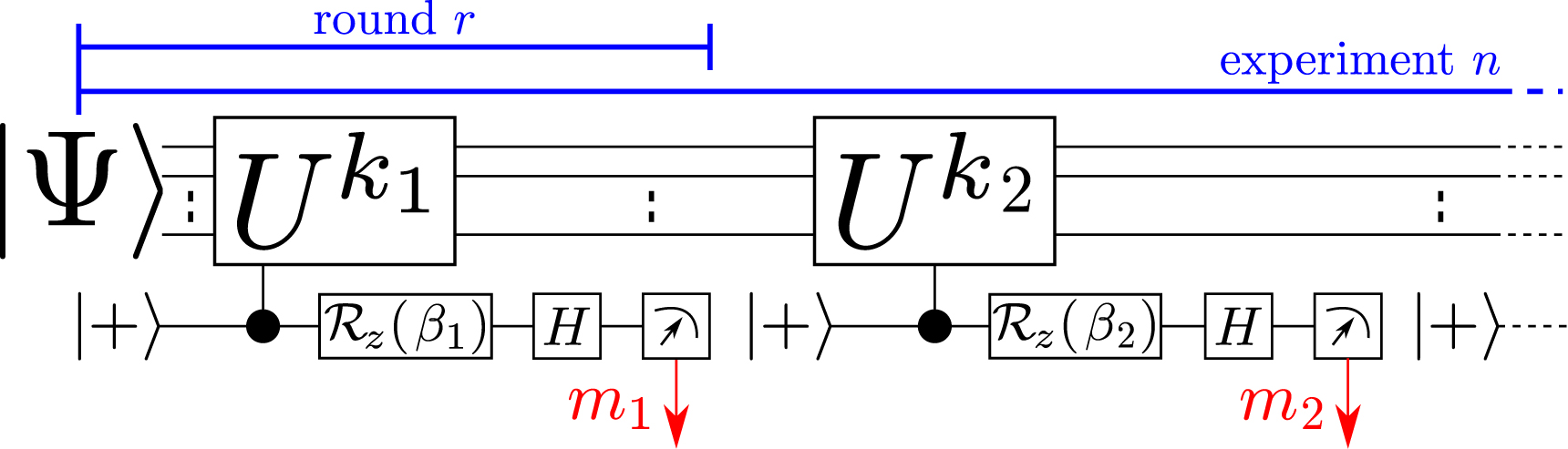
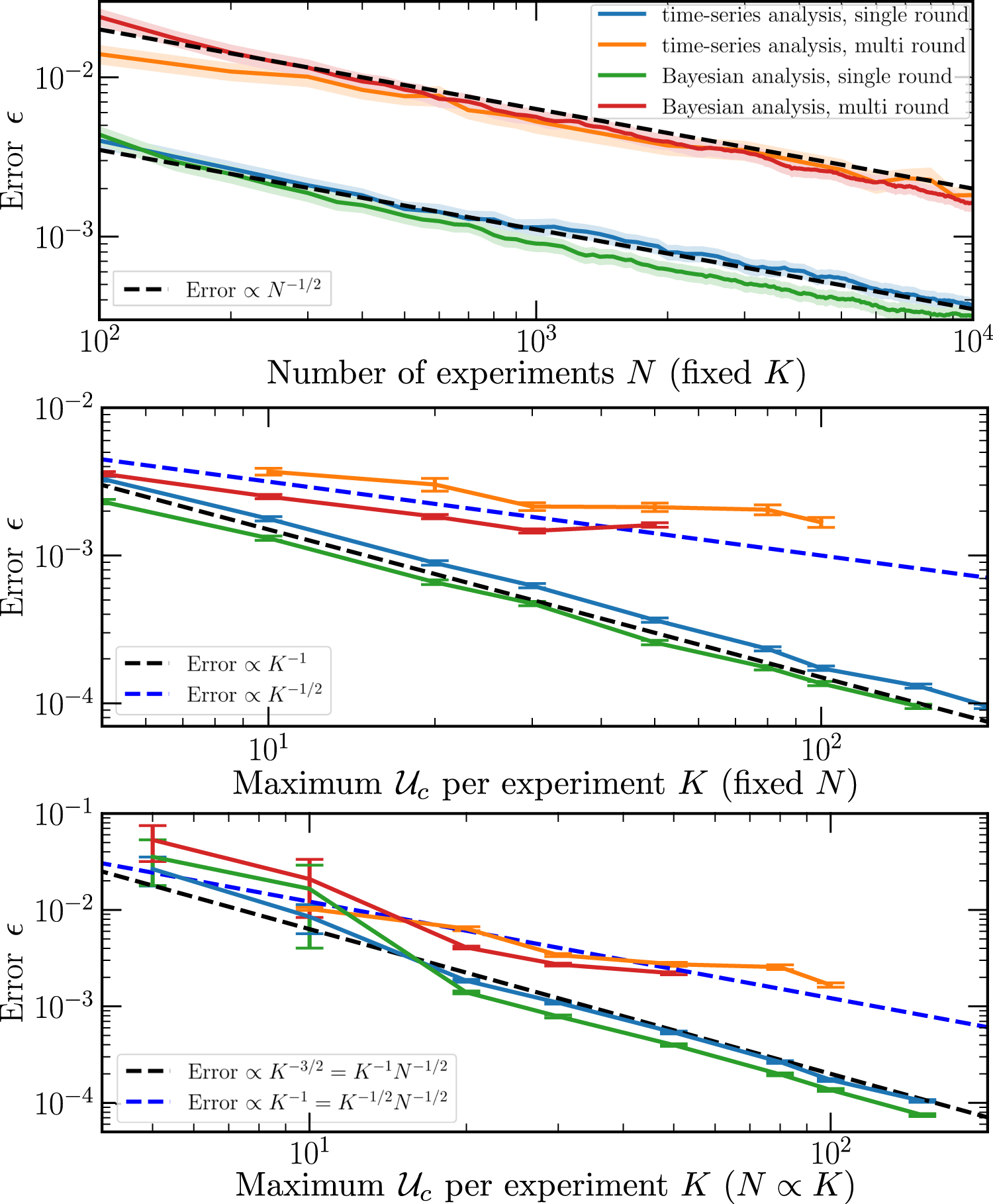
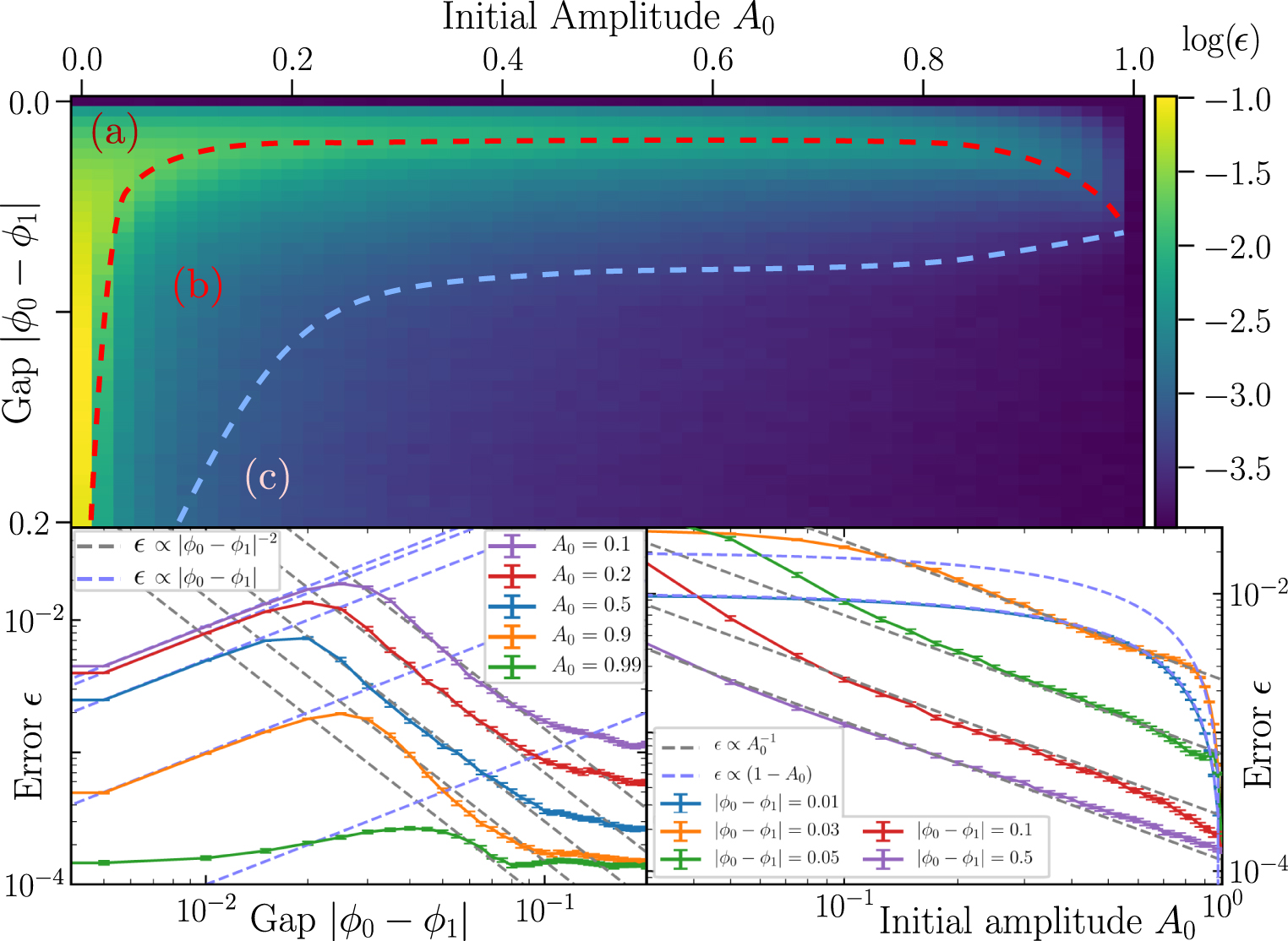
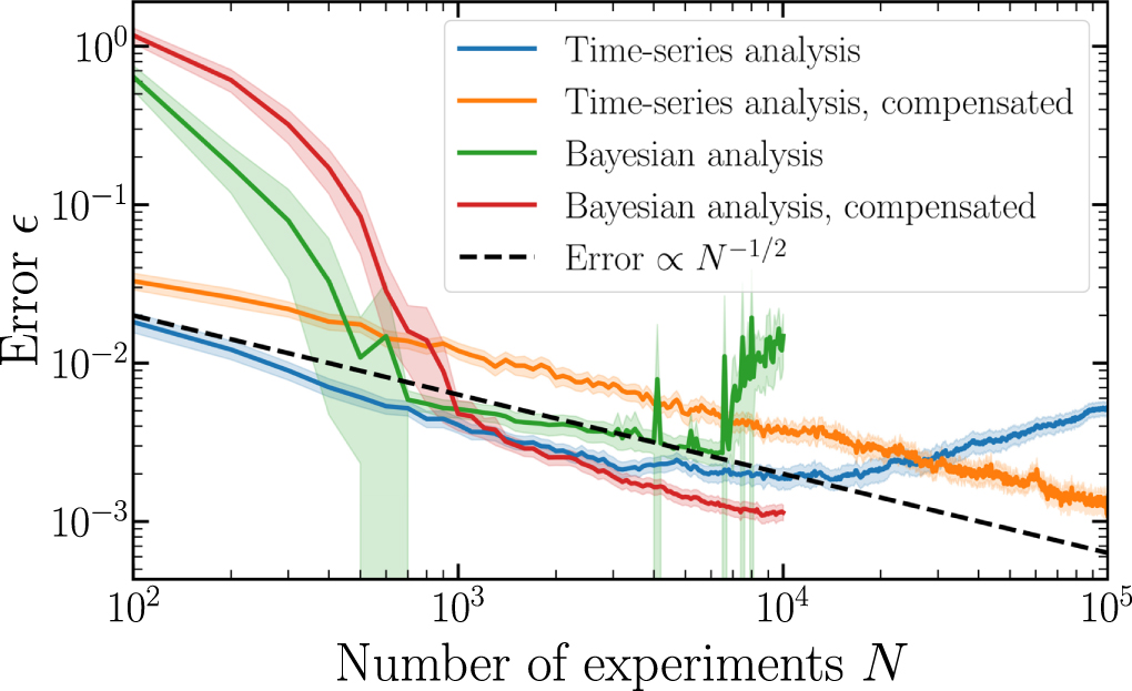
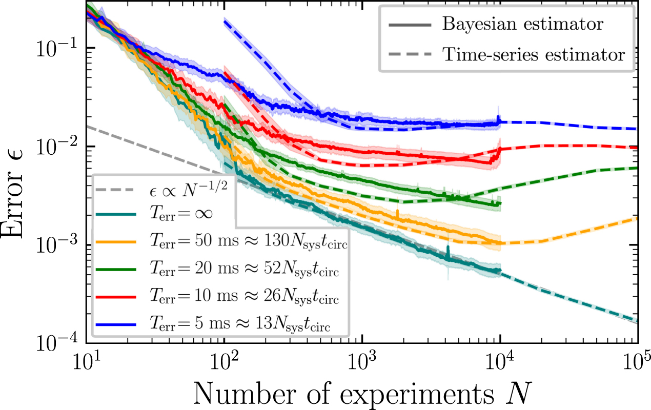