


Abstract
We present a general framework for modeling a wide selection of flocking scenarios under free boundary conditions. Several variants have been considered—including examples for the widely observed behavior of hierarchically interacting units. The models we have simulated correspond to classes of various realistic situations. Our primary goal was to investigate the stability of a flock in the presence of noise. Some of our findings are counter-intuitive in the first approximation, e.g. if the hierarchy is based purely on dominance (an uneven contribution of the neighbors to the decision about the direction of flight of a given individual) the flock is more prone to loose coherence due to perturbations even when a comparison with the standard egalitarian flock is made. Thus, we concentrated on building models based on leader-follower relationships. And, indeed, our findings support the concept that hierarchical organization can be very efficient in important practical cases, especially if the leader-follower interactions (corresponding to an underlying directed network of interactions) have several levels. Efficiency here is associated with remaining stable (coherent and cohesive) even in cases when collective motion is destroyed by random perturbations. The framework we present allows allows the study of several further complex interactions among the members of flocking agents.
Export citation and abstract BibTeX RIS

Original content from this work may be used under the terms of the Creative Commons Attribution 3.0 licence. Any further distribution of this work must maintain attribution to the author(s) and the title of the work, journal citation and DOI.
1. Introduction
Collective behavior is a very important aspect through which small or large groups of organisms optimize their living [1]. It involves collective decision making an various contexts, such as searching for food, navigating towards a distant target [2–5] or deciding when and where to go [4, 6–8]. Flocking is perhaps the most common and spectacular manifestation of collective behavior not only in nature since recently has gained attention in the context of collective robotics as well [9–11]. Most of the experimental and modeling approaches aimed at describing flocking by assuming egalitarian interactions among the members of a flock.
However, just as flocking is a widespread behavioral pattern of a collective, the hierarchical structure of the interactions among the members of groups is also very common [12]. Thus, starting with a trend-setting paper of Couzin et al [13] the question of leadership during flocking has attracted increasing interest. Early works assumed a two-level hierarchy while recent experimental observations involving some sophisticated animal groups such as pigeons or primates point towards the possibility of significantly more complex internal organization principles during group motion [2, 8, 14, 15]. In socially highly organized groups beyond a given size (dozens or so) the roles related to leadership do not seem to be simply binary, but several levels of hierarchy can be identified. In particular the available few experimental results indicate that many co-moving groups have an internal system of interactions which can be best interpreted in terms of pairwise hierarchical levels of interactions. Perhaps the best quantitatively evaluated hierarchical group motion was carried out for pigeon flocks [2, 16] in which a hierarchically distributed set of interactions was demonstrated using GPS tracks and a velocity correlation-delay method [2].
On the other hand, in spite of its relevance, there have been no realistic models proposed and studied devoted to the understanding of the conditions under which hierarchical flocking can be optimal. The only vaguely related original model is in a beautiful work by Shen [17], but the assumptions are quite arbitrary and the effect of the hierarchy on the performance of the flock is not investigated.
Therefore, our goal here is to design a general framework which allows the treatment of questions related to hierarchical leader-follower interactions in a general setting, when the flock is freely moving (in the present study in two dimensions). We also discuss the various variants allowed by our approach and characterize the efficiency of the behavioral rules by determining to what level a flock is stable against external perturbations. Hierarchy is thought to be prevalent because it can be shown to result in more efficient group performance [8, 12].
The present work is the first one in which a flexible and plausible framework is introduced to model hierarchical flocking. It turns out that introducing pairwise interactions satisfying a realistic hierarchical dynamics is far from being trivial. After introducing the model the main aspect we investigate is the stability of a flock moving freely in a border-less two-dimensional space. We shall associate with stability the tendency of a flock not to break into parts under external perturbations.
2. Definitions used in our model
For an egalitarian system, every particle is believed to be the same, while for a hierarchical system, individual difference exists. Any complex multi-agent system can be classified as egalitarian or hierarchical according to the set of pairwise relationships between any two individuals. For each pair of particles in an egalitarian system, both of them have the same ability (referring to the same contribution strength and bidirectional information flow) when making decisions for the next time step. Meanwhile, for each pair of particles in a hierarchical system, when making a decision, they may have different level of contribution to the decision (weight) or have a directed information flow relationship, like the leader-follower mechanism (follower has no influence on the behavior of the leader).
Graphs/networks represent a useful tool for visualizing these pairwise interaction relationships of individuals belonging to one co-moving group. Therefore, we define several matrices to describe the internal properties of the hierarchical mechanisms from different points of view, for the purpose of characterizing the differences between the egalitarian and hierarchical systems clearly.
2.1. Contribution matrix
Contribution matrix ![${C}_{N}={[{c}_{{ij}}]}_{N\times N}({c}_{{ij}}\gt 0)$](https://content.cld.iop.org/journals/1367-2630/21/9/093048/revision2/njpab428eieqn1.gif) is defined to describe the contribution strength (weight) of each particle during the decision making process regarding the new preferred directions of the particles.
is defined to describe the contribution strength (weight) of each particle during the decision making process regarding the new preferred directions of the particles.
- (i)For an egalitarian system, every particle has the same contribution value, that is, cij = q(q > 0), for i, j = 1, ⋯, N. q is a constant.
- (ii)For a hierarchical system, not all of these cij (
 ) have the same positive value. For example, cij = qi(qi > 0), for i, j = 1, ⋯, N, or cij satisfies some probability distribution(such as log-normal), for i, j = 1, ⋯, N. We name this kind of hierarchy as contribution driven hierarchical system.

2.2. Dominance matrix
The dominance matrix ![${B}_{N}={[{b}_{{ij}}]}_{N\times N}$](https://content.cld.iop.org/journals/1367-2630/21/9/093048/revision2/njpab428eieqn3.gif) is defined to describe the direction of information flow between each pair individuals. The direction of information flow specifies the set of particles whose behavior influences the decision of a given particle at each time step.
is defined to describe the direction of information flow between each pair individuals. The direction of information flow specifies the set of particles whose behavior influences the decision of a given particle at each time step.
- (i)For each pair of particles i and j () in an egalitarian system, their behaviors can be influenced by each other, that is to say, the information between each pair of particles is transmitted bidirectionally (corresponding to an undirected graph). Thus, in an egalitarian system for each pairwise interaction bij = bji = 1, ∀ i, j = 1, ⋯, N, .
- (ii)If the information flow of paired particles is directional, that is, only one particle can obtain the other particle's information (directed graph), then we have a dominance driven mechanism, which is another kind of hierarchy named dominance hierarchical system. For paired particle i and j, if i is led by j, then we have bij = 1 and bji = 0 (i, j = 1, ⋯, N,).
- (iii)If bii = 1(i = 1, ⋯, N), then BN is called dominance matrix. If bii = 0 (i = 1, ⋯, N), then BN is called strictly dominance matrix. We call the egalitarian system with bii = 0 (i = 1, ⋯, N) as strictly-egalitarian system. The egalitarian system discussed in this paper refers to the case that bii = 1 (i = 1, ⋯, N). We use the terminology dominance hierarchical system with bii = 0 (i = 1, ⋯, N) as dominance strictly-hierarchical system.


Leader-follower mechanism is a typical kind of dominance relation in hierarchical organizations. For each pair of particles, leader particle does not take into account the influence of the follower, but the follower considers the behavior of the leader particle when making decision on its behavior at the next step. This feature is represented by the fact that the matrix BN is not symmetric. Without loss of generality, we number these particles according to the level of dominance from 1 to N. Particle 1 is the strongest one of the whole system, while particle N is the weakest one. Therefore, the dominance matrix BN is a complete and symmetric matrix for egalitarian systems; for a dominance hierarchical system, BN with non-zero diagonal elements is a lower-triangular matrix; for dominance strictly-hierarchical system, BN is a strictly lower-triangular matrix (strictly triangular matrix refers to the triangular matrix whose diagonal elements are all zero).
2.3. Egalitarian versus hierarchical systems
Now we can give a formal definition of egalitarian and several kinds of hierarchical systems.
2.3.1. Egalitarian system
For each pair of individuals, if both of them will use each other's information with the same weight to decide the behavior at the next step, we say it is an egalitarian system. An egalitarian system satisfies the following two rules
- (i)cij = q, ∀ i, j = 1, ⋯, N, q is a positive constant;
- (ii).
2.3.2. Contribution driven hierarchical system
A contribution hierarchical system satisfies the following two rules.
- (i)cij follows some distribution for i, j = 1, ⋯, N (thus, not all of these cij have the same positive value);
- (ii)bij = 1, ∀ i, j = 1, ⋯, N.
2.3.3. Single-layer leader-follower hierarchical system (dominance driven hierarchical mechanism)
A single-layer leader-follower hierarchical system satisfies the following two rules.
- (i)cij = q, ∀ i, j = 1, ⋯, N, q is a positive constant;
- (ii).
2.3.4. Single-layer leader-follower strictly-hierarchical system (dominance driven strictly-hierarchical mechanism)
A single-layer leader-follower strictly-hierarchical system satisfies the following two rules.
- (i)cij = q, ∀ i, j = 1, ⋯, N, q is a positive constant;
- (ii).
2.3.5. Double-layer leader-follower hierarchical system (contribution driven dominance hierarchical mechanism)
In case the weights in the contribution matrix are not equal, we associate the system with the presence of dominance (the contribution of agents having a larger weight dominate over the contribution by those with a smaller weight). We consider such systems whose behavior is determined through a contribution driven mechanism. Then, the particle with larger weight contribution is named as leader, while the other one is named as follower. A double-layer leader-follower hierarchical system satisfies the following two rules:
- (i)cij follows some distribution for i, j = 1, ⋯, N (but not all of these cij have the same positive value);
- (ii)bij = 1, i ≥ j, i, j = 1, ⋯, N.
2.3.6. Double-layer leader-follower strictly-hierarchical system (contribution driven dominance strictly-hierarchical mechanism)
A double-layer leader-follower strictly-hierarchical system satisfies the following two rules.
- (i)cij meets some distribution for i, j = 1, ⋯, N (but not all of these cij have the same positive value);
- (ii)bij = 1, i > j, i, j = 1, ⋯, N.
The above systems can be characterized by their intersection matrix  . For an egalitarian system, it is a complete matrix with the same elements. For contribution hierarchical systems, it becomes a complete matrix with various elements. For single-layer leader-follower hierarchical system, it is a lower-triangular matrix with the same lower-triangular elements. For single-layer leader-follower strictly-hierarchical system, it is a strictly lower-triangular matrix with the same lower-triangular elements. For double-layer leader-follower hierarchical system, it becomes a lower-triangular matrix with varying lower-triangular elements. For double-layer leader-follower strictly-hierarchical system, it becomes a strictly lower-triangular matrix with varying lower-triangular elements.
Besides, in a more general model, cij and bij can be time-dependent. If cij and bij is not time-dependent that means everyone in the system has fixed a set of relationships. If cij(t) and bij(t) are time-dependent, then the relationships among these particles changes with time. Other different variants can thus be defined according to the contribution matrix cij(t) and dominance matrix bij(t). Here, we only discuss the case that when cij and bij are constant.
3. Hierarchical model for flocking
We consider in this paper N particles moving continuously (off lattice) in a free area without any boundary limitation. As shown in figure 1, the position and direction of N particles at the beginning are generated randomly, while over time these particles are expected to move coherently (ordered state). The figure is for the noiseless case.
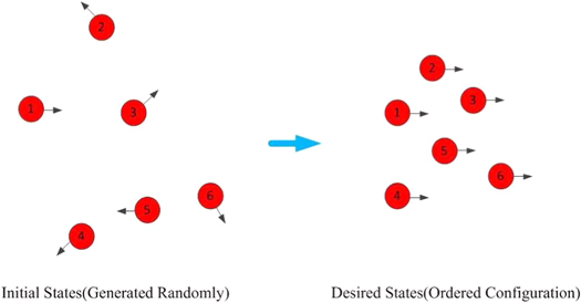
Figure 1. Initial configuration versus the ordered phase of collective motion.
Download figure:
Standard image High-resolution imageSuppose that the time interval between two updates of the directions and positions is Δt = 1. This assumption can be made without loosing generality since Δt occurs only in combination (being multiplied by it) with velocity terms At t = 0, N particles were randomly distributed within an area of a given size and have the same absolute velocity υd as well as randomly distributed directions θ. At each time step, the position of the ith particle is updated according to

In each time step, the velocity of a particle vi(t + 1) is updated according to the following equation

where  is the alignment term,
  is the repulsion term, and
  is the attraction term.
The alignment term was constructed to have an absolute value υ and a direction given by the angle  . The angle was obtained from the expression

where Δθ(t) represents noise, which is a random number chosen with a uniform probability from the interval [−η/2, η/2].  denotes the average direction of the velocities of neighbors of the given particle i. The average direction is given by the angle

Neighbor matrix ![${L}_{N}(t)={[{l}_{{ij}}(t)]}_{N\times N}$](https://content.cld.iop.org/journals/1367-2630/21/9/093048/revision2/njpab428eieqn16.gif) describes the neighbor relationships of particles at time t, where
describes the neighbor relationships of particles at time t, where

The definition of adjacency matrix ![${A}_{N}(t)={[{a}_{{ij}}(t)]}_{N\times N}$](https://content.cld.iop.org/journals/1367-2630/21/9/093048/revision2/njpab428eieqn17.gif) is
is

where  . Here, r denotes the interaction radius. Using the above expressions the alignment term can be written as

where calign is the coefficient of the alignment term. ei(t) is a unit vector with direction angle  .
.
The repulsion term exists only when the distance between any two particles is smaller than the repulsive radius rrep. And the repulsion term is defined as

where  and
and  is the coefficient of the repulsion term.
The attraction term is only considered for the boundary particles [18] of the whole system when the distance between two particles is between rrep and radh.

where  and
and  is the coefficient of the attraction term. This term is introduced in order to prevent the flock spreading (or, in other words, 'evaporating') due to perturbations.
Figure 2 shows the neighbour matrix of several variants of flocks mentioned in the last section. From figure 2, visualizes the differences between the egalitarian system from the typical hierarchical systems.
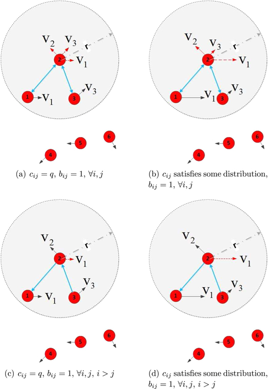
Figure 2. Neighbor matrix. (a) egalitarian system; (b) contribution driven hierarchical system; (c) single-layer leader-follower strictly-hierarchical system; (d) double-layer strictly-hierarchical system. For each figure, only those velocity vectors which are marked by red arrows will be used to calculate the velocity of particle 2 at the next step.
Download figure:
Standard image High-resolution image4. Simulations and discussion
The simulations were carried out in a free two-dimensional area. We considered groups of particles having various sizes ranging from 10 to 1280 particles. In order to keep the continuity and comparability of these simulation results of different group sizes, we chose the scale of the area for the random initial positions directly proportional to the scale of group size N, and generated the initial angle from the interval (−π, π]. Here, without loss of generality, the random initial positions are generated from a rectangle area with length L and width 0.6L. Then, the initial density of the system  , which is constant for various group sizes. We aimed at comparing the stability of egalitarian systems versus various hierarchical systems for varying levels of external disturbances (noise) and for different group sizes.
The alignment item of egalitarian flock model is much like the self propelled particle model proposed by Vicsek et al in 1995 [19], where the definition of neighbors of particle i includes itself and the contribution of the particles is the same. Thus, we call the egalitarian model as VEM (E for egalitarian, M for model). The contribution driven hierarchical model is called as CHM (C for contribution).
According to the definition of the strictly dominance matrix BN, the neighbor matrix of a dominance-related strictly-hierarchical system has zero-value diagonal elements, that is, we have lii = 0, ∀ i = 1, ⋯, N for all dominance-related strictly-hierarchical systems. lii = 0 means that the neighbor set of particle i does not contain itself. In the following under hierarchy, we always mean hierarchical leader-follower kind of hierarchy. Therefore, we name the single-layer leader-follower hierarchical model ( ) as SHM (S for single-layer leader-follower), and we call the single-layer leader-follower strictly-hierarchical model by SHMZ (S for single-layer leader-follower, and Z for lii = 0, ∀ i = 1, ⋯, N). Similarly, the double-layer leader-follower strictly-hierarchical flock model (lii = 0, ∀ i = 1, ⋯, N) is named as 'Double Hierarchical Model with Zero-s (DHMZ)', while when
  , we call it 'Double Hierarchical Model (DHM)'.
4.1. VEM versus CHM/SHM
In these simulations, we used  , and interaction radius r = 1.1.
4.1.1. Order parameter
For this case we used the average normalized velocity as the order parameter, defined as

where T = 2000 is the simulation time for each experiment.
The error bar is defined as:

where  is the standard deviation of the order parameter values, and n > 0 is the number of simulations for a given system size. The typical values of n were chosen as follows:
4.1.2. Results
First, we compared the stability of VEM and some simple hierarchical flocking systems, such as CHM and SHM. According to our results (see figures 3 and 4), a simple dominance-based system does not perform better than the much studied egalitarian flock. It should be noted that we did not compare VEM with CHM/SHM for larger group sizes than N = 160, because we guess CHM/SHM still do not perform better than VEM, but readers who are interested in size dependence are welcome to investigate it.
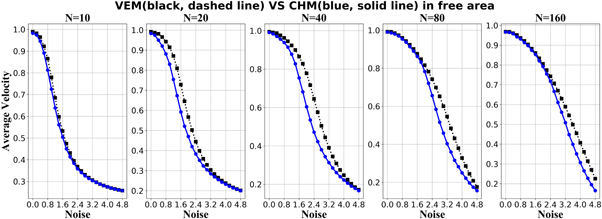
Figure 3. Quantitative comparison of VEM and CHM ( , for i = 1, ⋯, N) for various group sizes. cij satisfies log-normal distribution (whose mean is 0 and standard deviation is 1) for the CHM system. Note that both figures 3 and 4 show that the egalitarian system is more stable than the simple dominance-based (referring to contribution) hierarchical system.
Download figure:
Standard image High-resolution image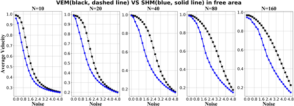
Figure 4. Quantitative comparison of VEM and SHM ( , for
, for  ) for various group sizes. cij = q(q > 0) for the SHM system.
Download figure:
Standard image High-resolution image4.2. VEM versus DHM/DHMZ
In this simulation, we use  , and interaction radius r = 2.2.
4.2.1. Order parameter
As mentioned above, we shall associate the stability with the tendency of a flock not to break into parts under external perturbations. In order to measure the stability of the particle group, we used the following velocity correlation as the order parameter

where  means
means  and
and  . This expression indicates the stability of the flock under different conditions. We did not use the average velocity as the order parameter here, just because velocity correlation (as order parameter) could offer a more strictly stability description when the system is divided into two or more coherently moving subgroups.
4.2.2. Results
We compare VEM with DHM and DHMZ separately. figure 5 shows the comparison results of the VEM and DHM, while figure 6 shows the comparison results of VEM and DHMZ.
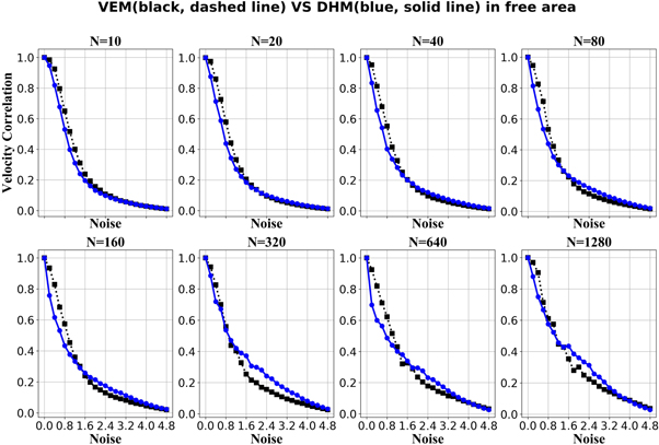
Figure 5. Quantitative comparison of VEM and DHM ( for i ∈ 1, ⋯, N) for various group sizes. cij satisfies log-normal distribution(whose mean is 0 and standard deviation is 1) for DHM.
Download figure:
Standard image High-resolution image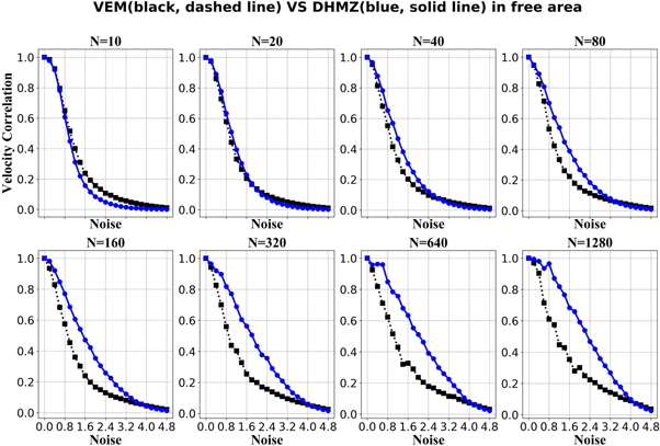
Figure 6. Quantitative comparison of VEM and DHMZ (lii = 0 for i ∈ 1, ⋯, N) for various group sizes. cij satisfies log-normal distribution (whose mean is 0 and standard deviation is 1) for DHMZ.
Download figure:
Standard image High-resolution imageAccording to figure 5, we can see that VEM is a little bit better (better meaning that it is more ordered for the same amount of noise) than the DHM for different group size under lower noise, while it seems that DHM is a little better than VEM under larger noise. However, the advantage is so small that can be ignored. At the same time, it seems that there exists no relevant difference among the simulation results for various group sizes.
Figure 6 demonstrates that the DHMZ hierarchical model is significantly more stable than an egalitarian model for flocking, and the advantage is increasingly obvious as the size of the system increases. However, the stability gap between an egalitarian flock and a hierarchical flock stops increasing from 320 to 1280 particles. That is to say, the difference in the performances between the egalitarian system and the hierarchical system is increasing with system size, but only up to a given flock size and is not changing as the group size reaches a certain threshold. This is quite along the intuitive picture which suggests that hierarchy may play a relevant role only up to—at most—a few hundred of flock members.
At first, we were puzzled by the result that DHMZ performs much better than DHM. However there exists a plausible interpretation. The zero on the diagonal means that a unit does not consider its own decision (direction) when it decides about its direction at each time step. The element on the diagonal being not zero means that when a unit makes a decision, it will implement the average decision of both itself and its neighbors. In short, an interaction matrix with zeros along the diagonal means that the 'follow the leaders' principle is manifested in an enhanced way. Even if in other interactions the given unit is usually a leader (having a relatively large bij or cij values), when this leader decides how to proceed, it becomes a follower in relation with the others.
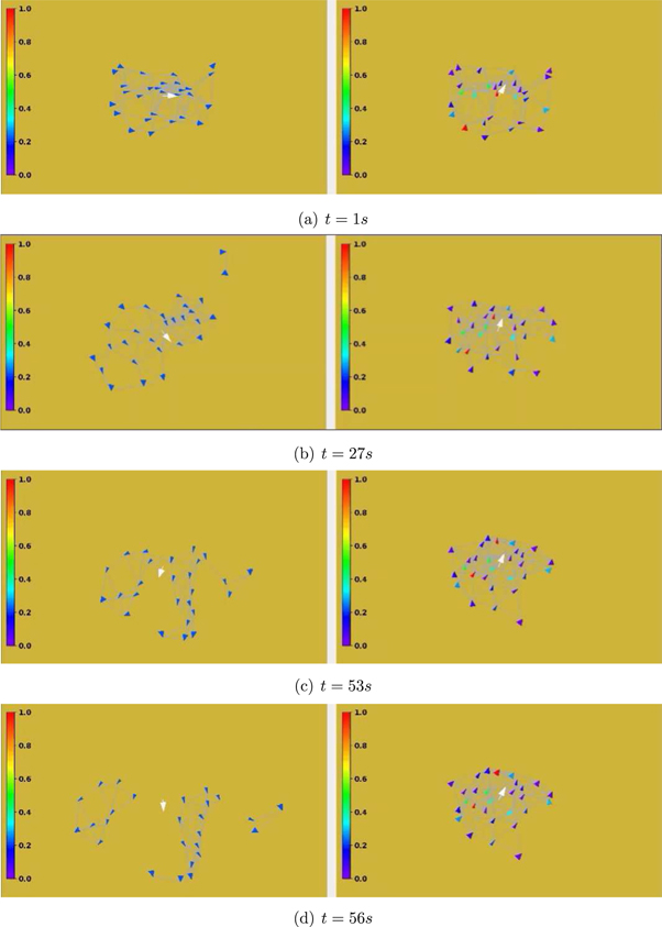
Let us consider twenty-eight particles, for example, figure 7 shows some important scenarios during the flocking process. The color bar reveals the weight of the contribution of the given particle. For example, the red particle is the strongest one, while the purple one is the weakest particle. The contribution values of these particles belonging to the DHMZ system satisfy log-normal distribution. That is, cij, i, j = 1, ⋯, N, i > j satisfy log-normal distribution, with mean value 0 and standard deviation 1. At the same time, the contribution value of each particle belonging to VEM system is equal, and the sum of the contribution values of VEM system is equal to the sum of the contribution values of the DHMZ system. The initial state of the twenty-eight particles in VEM is the same as that in DHMZ. In figure 7, the boundary particles are indicated by a bigger size than the inside particles. The first picture in figure 7 displays the state of all the particles at start. The left part of figure 7(b) depicts the structure of the VEM flock being less cohesive than the DHMZ (the right one) and a couple of particles are already separated from the VEM flock. Figures 7(c) and (d) show two key moments when VEM results in three separated groups while DHMZ results still in a single cluster. This can be taken as an important evidence to demonstrate that leader-follower hierarchical systems are more efficient regarding their stability against perturbations which the individual units are subject to.
Figure 7. VEM and DHMZ for twenty-eight particles flocking. For each scenario, the left one is VEM, while the right one is DHMZ. (a) the scenario at time t = 1 s. (b) the scenario at first separate time t = 27 s. (c) the scenario at time t = 53 s. (d) the scenario at the second separate time t = 56 s.
Download figure:
Standard image High-resolution image
5. Conclusions
In conclusion, we have introduced an interpretation of the possible behaviors of interacting, collectively moving units (let it be birds, fish or people, etc) which is more general than any of the ones we are aware of. The main feature of our approach is that it unites into a single formalism the results and assumptions of the prior models and observations. Some of our results are plausible: a simple averaging of the direction of motion of neighbours (VEM) is quite efficient when the efficiency is measured as the level of stability against external/internal perturbations. The main points of our paper are concerned with the role of hierarchy among the co-moving units. We have located two non-trivial models: (i) the contribution during the averaging of the directions is weighted, (ii) the given unit is—when evaluating its direction in the net time step—in a fully 'follower mode' (DHMZ). At first, our numerical findings (i) is inefficient, (ii) performs the best, looked as ssurprising, but we provided the interpretations for these findings. Our formalismis general enough for using it to introduce a large family of more specific models.
Acknowledgments
This work was partly supported by the following grants: U.S. Air Force, Office of Scientific Research grant no. FA9550-17-1-0037; H2020, EU FP7 RED-Alert No: 740688 and the (Hungarian) National Research, Development and Innovation Office grant No K128780.