

Abstract
Finite-amplitude supernonlinear electron-acoustic waves (EAWs) are investigated under the nonlinear Schrödinger (NLS) equation in a plasma system that is composed of cold electron fluid, immobile ions and q-nonextensive hot electrons. Using the wave transfiguration, the NLS equation is deduced in a dynamical system. The presence of finite-amplitude nonlinear and supernonlinear EAWs is shown by phase plane analysis. The effects of the nonextensive parameter (q) and the speed of waves (v) on different traveling wave solutions of EAWs are presented. Furthermore, by introducing a small external periodic force in the dynamical system, multistability behaviors of EAWs under the NLS equation are shown for the first time in classical plasmas.
Export citation and abstract BibTeX RIS
1. Introduction
The study of nonlinear wave propagation (such as solitons, envelope waves, shocks, vortices, etc.) is one of the most interesting subject in the realm of plasma physics [1–4]. The properties of different nonlinear modes of wave propagation in electrostatic and magnetized plasma media have been studied by many researchers [5–8]. Solitary structures would be created because of the balance between nonlinearity and dispersion effects [7, 9]; solitary waves of this kind are well known as Korteweg de–Vries (KdV) solitons [10]. Generally, there are two different kinds of nonlinear structure in plasma media: one is KdV and the other is an envelope soliton, which is formed when the group dispersion of a wave balances out the nonlinearity of the medium. The dynamics of the former are governed by the KdV equation and those of the latter by the nonlinear Schrödinger (NLS) equation [11, 12].
EAWs are electrostatic modes with high frequency relative to the plasma frequency of ions [13]. The concept of EAWs was first introduced by Fried and Gould [14]. They found that besides ion-acoustic and Langmuir waves, other highly damped acoustic waves (called EAWs) may exist that differ significantly from the first two [14–16]. Electrostatic waves of this type can propagate in magnetized [17, 18] and unmagnetized plasma [19, 20]. Generally, EAWs consist of electrons at two different temperatures, i.e. hot and cold electrons. Ions and cold electrons play the inertial role and remain motionless to form a neutralizing background while the hot electrons are effective in producing a restoring force for EAWs. The inertia of ion-acoustic waves (IAWs) comes from the heavy ions [21, 22]. So, the phase velocity of EAWs is the thermal velocity between hot and cold electrons. Dubouloz et al [23, 24] have experimentally reported EAWs in both one-dimensional magnetized and unmagnetized collisionless plasma with immobile ions, cold electrons and Maxwellian hot electrons. In fact, since the hot electrons have been trapped in a wave potential and have formed phase space holes, the hot electrons cannot obey a Maxwellian distribution [25]. Accordingly, in the present work, we shall suppose stationary ions, cold electrons and q-nonextensive hot electrons in plasma media. The q-nonextensive distribution is a generalization of the Cairns nonthermal distribution and it has been extensively applied in systems enriched with long-range interactions [26–29]. The features of propagation of linear and nonlinear EAWs in unmagnetized plasma have been studied by numerous researchers [30–34]. For instance, Saha et al [8] discussed the qualitative structures of EAWs in an unmagnetized plasma, applying the concept of dynamical systems and obtaining all plausible phase portraits with solitary and periodic wave solutions. They found that parameters such as the nonextensive parameter (q), the number density ratio of hot and cold electrons (α) and the speed of the wave (v) show significant impact on dynamical motions of EAWs. Demiray [15] considered a plasma medium with hot electrons following a kappa distribution, cold electrons and immobile ions to study EAWs. He used the reductive perturbation technique (RPT) to study the modulational stability for all admissible wavenumbers. Recently, Fahad et al [35] investigated the generalized dispersion properties of EAWs for isotropic, non-relativistic, degenerate/non-degenerate plasmas using the longitudinal response functions in the presence of quantum recoil.
A supernonlinear wave (SNW) is a recently developed wave introduced by Dubinov and Kolotkov [36]. They classified SNWs on the grounds of considerable topology of their phase spaces. The existence of SNWs can be examined in plasmas with three or more components [37–39]. Many works [8, 40, 41] have studied arbitrary SNWs using the Sagdeev potential function. But, using the bifurcation theory, Saha et al [42–44] presented arbitrary supernonlinear periodic waves for the first time. Very recently, small-amplitude superperiodic IAWs under the modified KdV equation [45, 46] and modified Gardner equation [46] have been reported. However, small-amplitude supernonlinear EAWs have not been studied applying the bifurcation theory under the NLS equation. Some nonlinear systems show more than one nonlinear dynamical property for a group of parameters at different initial conditions. Such a property is known to have multistability behavior. The multistability plays a significant role in determining the nonlinear behaviors of physical systems [47, 48]. Experimentally, such behavior was first observed in a Q-switched gas laser [49]. Therefore, multistability is a fresh area of research in nonlinear plasma systems and hence more research is needed. In the current study, we examine the amplitude modulation of EAWs in a plasma consisting of stationary ions, a cold electron fluid and q-nonextensive hot electrons. The nonlinear Schrödinger equation is considered as the evolution equation for the study of EAWs. We investigate the qualitative dynamical features of the EAWs applying the concept of planar dynamical systems. In addition, we examine the multistability behaviors of the dynamical system for the EAWs.
The article is organized as follows. In section 2, governing equations are discussed. In section 3, the NLS equation is considered and dynamical properties of EAWs are examined through phase plane analysis. In section 4, multistability behavior of the system is examined under the impact of an external force. Lastly, in section 5, conclusions of the study are drawn.
2. Governing equations
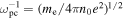
We consider a homogeneous plasma composed of immobile ions, a cold electron fluid and hot electrons following a nonextensive distribution. The following governing equations characterize the motions of EAWs:


where n and ne stand for cold and hot electron number densities. Here,  . We have u as the velocity of cold electrons and ϕ as the electrostatic wave potential. Here, Th denotes the temperature of hot electrons, mh stands for electron mass, e denotes the charge of electrons and kB refers to the Boltzmann constant. Here, t and x denote time and space variable, respectively. The entities in this plasma system are normalized as follows: n is normalized to n0 and u is normalized by
  . Here, ϕ, t and x are normalized by
  ,
,  and
and 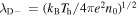 , respectively.
The following nonextensive distribution function is formed to represent the velocity distribution of electrons:
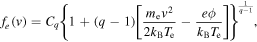
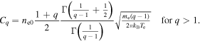
where parameters Te and q are the temperature of electrons and the nonextensive parameter, respectively. The function fe(v) generalizes the Tsallis entropy and also follows the law of thermodynamics. Now, Cq representing the normalization constant is expressed as
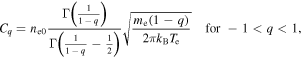
and
To obtain the nonextensive electron number density, the function fe(v) is integrated over all velocity ranges. Then, we obtain

After normalization, the number density of hot electrons [50] following the q-nonextensive distribution reduces to

3. The NLS equation and dynamical properties of EAWs
To study small-amplitude EAWs, the NLS equation is derived using the RPT, for which the following stretching coordinates are considered for the independent variables:

and the expansions are considered for the dependent variables are

with  as a small parameter (0 < ≪ 1) and V as the group velocity of the wave. The 3D NLS equation is considered as

where  . The dispersion coefficient P and the nonlinear term Q are expressed as

where  ,
,  ,
,  ,
,  ,
,  ,
,  and
and  . Here, one can refer to the work [50] for derivation of the NLS equation.
To investigate dynamical behaviors of EAWs, we consider transformations  and
and 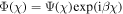 in the NLS equation (7). Then, we obtain

where 0 < l < 1 and v is the speed of the traveling wave. Equating the real part of equation (8) to zero, we obtain the equation

We represent equation (9) as the following dynamical system
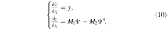
where  and
and  . The Hamiltonian function
  of the dynamical system (10) is given by

and we obtain
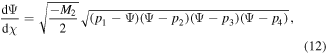
where  and p4 are roots of
  , where
  and
and  is a point on the phase plane. The relation (12) gives the traveling wave solution of the plasma system for the orbit through the point
  . Now, we consider the system (10) as
  then
then
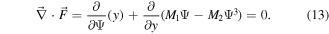
Equation (13) shows that the system (10) is a conservative dynamical system.
The dynamic motions of the system are analyzed through phase plane analysis. The phase plane analysis shows that the system (10) contains three fixed points Fi at (Ψi,0), where i = 0, 1, 2. From the relation H(Ψ, y) = 0 at F0, we obtain nonlinear homoclinic trajectories, which correspond to nonlinear solitary wave solutions. The nonlinear homoclinic trajectories enclosing fixed points F1 and F2 are associated with nonlinear solitary wave solutions of the plasma system. The relation H(Ψ, y) = hi around the fixed points F1 and F2 corresponds to nonlinear periodic trajectories that are associated with nonlinear periodic wave solutions of the plasma system. Therefore, we obtain rarefactive and compressive electron-acoustic solitary wave solutions corresponding to negative and positive regions of homoclinic trajectories in the phase plot of figure 1. We also encounter a new class of EAWs in the form of a periodic wave enclosing the three fixed points F0, F1 and F2 with one separatrix. This periodic wave belongs to a class of superperiodic waves. The existence of small-amplitude superperiodic EAWs through bifurcation in the framework of the NLS equation is being reported for the first time.
It is important to note that the ranges of q are  and q > 1. However, through the recent reports [51, 52], the acceptable range of q in the case of superextensivity reduces to 1/3 < q < 1, such that the physical condition of energy equipartition is satisfied. Therefore, we restrict our study to the range 1/3 < q < 1 of the nonextensive parameter q.
We presents phase plots of the system (10) in figure 1 for q = 0.5 with α = 1.5, β = 0.2, l = 0.3, k = 0.3 and v = 0.2 . Here, NPT1,0 and SPT3,1 denote a nonlinear periodic trajectory and a supernonlinear periodic trajectory, respectively. The nonlinear homoclinic trajectory is represented by NHT1,0.
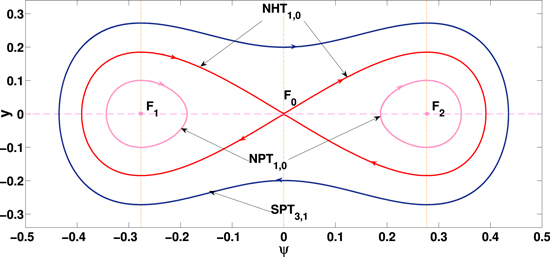
Figure 1. Phase plot of equation (10) for q = 0.5 with α = 1.5, β = 0.2, l = 0.3, k = 0.3 and v = 0.2.
Download figure:
Standard image High-resolution imageNumerically, we obtain different EAW solutions corresponding to the phase plot, which are shown in figure 2. We present the variations of a nonlinear periodic wave in figures 2(a) and (b) and those of a supernonlinear periodic wave in figures 2(c) and (d) with respect to changes in parameters q and v. It is clear from figures 2(a) and (c) that for higher q values, the amplitude of nonlinear periodic waves grows and their width decays, while both the width and amplitude of superperiodic EAWs decay. When the speed of the wave (v) is increased, the amplitude of a nonlinear periodic wave decreases and its width increases, while the amplitude of a superperiodic EAW grows and its width decays as seen in figures 2(b) and (d).
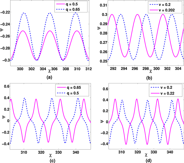
Figure 2. Nonlinear periodic solutions with variation of (a) q and (b) v, and supernonlinear periodic solutions with variation of (c) q and (d) v while other parameters are the same as in figure 1.
Download figure:
Standard image High-resolution imageThe solitary wave solution of EAWs is obtained as

Here, positive and negative signs in solution (14) correspond to compressive and rarefactive electron-acoustic solitary wave (EASW) solutions. We show differences in compressive and rarefactive EASWs by varying q and v in figures 3(a)–(d). It can be easily observed that compressive and rarefactive EASW solutions decay as q increases. However, the amplitude of EASWs grows and their width diminishes with higher values of v.
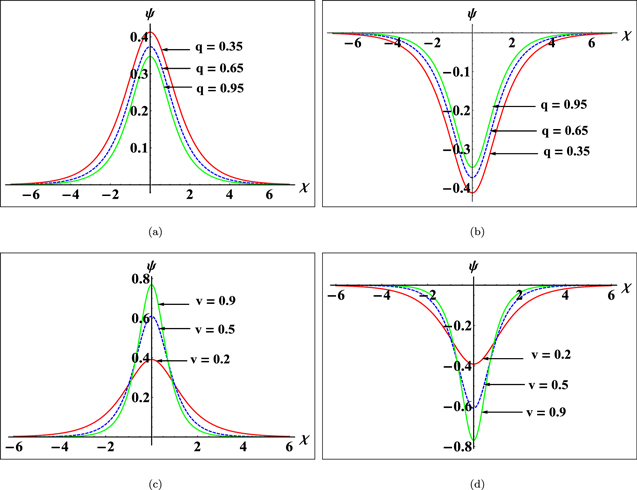
Figure 3. Variations of (a) compressive and (b) rarefactive EASWs by changing q, and variations of (c) compressive and (d) rarefactive EASWs by changing v while other parameters are same as in figure 1.
Download figure:
Standard image High-resolution image4. Multistability
Perturbation of the source in nonlinear systems acts as an external driving force. Lately, Mandi et al [53] reported nonlinear waves under the impact of source perturbation. For this study, we consider f0cos(Ωχ) as an external periodic force with f0 as its strength and Ω as its frequency. Thus, we deduce the dynamical system (10) by introducing f0cos(Ωχ) into the perturbed dynamical system (15) as

The nonlinear system expressed by equation (15) shows interesting dynamical phenomena, such as the existence of two or more attractors just by varying initial conditions. Such an interesting phenomenon is called multistability or coexisting attractors. Here, we consider only the variations of initial conditions to examine the existence of various attractors in the system (15) with different Ω and f0 while other system parameters are fixed as in figure 1. For this study, we present the existence of multistability for EAWs from the system (15) through phase spaces and their corresponding time series plots.
We present the coexistence of quasiperiodic and periodic attractors for f0 = 0.02 and Ω = 0.05 with q = 0.5, α = 1.5, β = 0.2, l = 0.3, k = 0.3 and v = 0.2 in figure 4. Here, for a lower impact of external force, we observe a torus-like pattern of a quasiperiodic attractor at initial condition [0.3, 0] (green) and one periodic attractor at [0.8, 0] (purple). This multistability behavior of the system (15) can be depicted by their respective time series plots in figures 4(c) and (d).
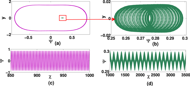
Figure 4. (a) Periodic motion and quasiperiodic motion at initial conditions [0.8, 0] (purple) and [0.3, 0] (green). (b) Enlarged view of the phase plot of quasiperiodic motion. Also shown are time series plots of (c) periodic motion in purple and (d) quasiperiodic motion in green for f0 = 0.02, Ω = 0.05 with q = 0.5, α = 1.5, β = 0.2, l = 0.3, k = 0.3 and v = 0.2.
Download figure:
Standard image High-resolution imageIn figure 5, it is interesting to observe two types of quasiperiodic behavior for the system (15) at the different initial conditions [0.077, 0] (light blue) and [0.09, 0] (magenta) under the influence of an external periodic force with f0 = 0.6, Ω = 3 and other parameters fixed as in figure 4. Here, the existence of two types of quasiperiodic motion is depicted by their corresponding time series plots in figure 5(b) in their respective colors.
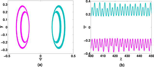
Figure 5. (a) Two types of quasiperiodic motions at initial conditions [0.077, 0] (light blue) and [0.09, 0] (magenta), and (b) corresponding time series plots for f0 = 0.6 and Ω = 3 with other parametric values the same as in figure 4.
Download figure:
Standard image High-resolution imageThe coexistence of different quasiperiodic motions with different initial conditions is shown in figures 6(a) and (c) for f0 = 0.6, Ω = 3 and other parametric values the same as in figure 4. The generation of such behavior indicates the multistability behavior of EAWs for the system (15). Here, figure 6(a) shows the existence of loop-forming quasiperiodic motions at initial condition [0.09, 0.55] (red), while a torus-like structure of quasiperiodic behavior is obtained at [0.085, 0.55] (blue). However, in figure 6(c), we encounter three different quasiperiodic motions showing a torus-like pattern at initial condition [0.08, 0.009] (blue), a four-loop pattern at [0.08, 0.9] (red) and a three-loop pattern at [0.099, 0.99] (green). These features of quasiperiodic motions of the system (15) are evident from their respective time series plots shown in figures 6(b) and (d).
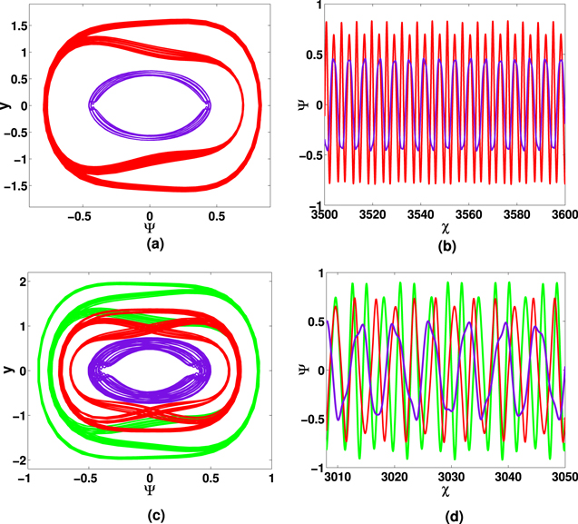
Figure 6. (a) Two types of quasiperiodic motion at initial conditions [0.085, 0.55] (blue) and [0.09, 0.55] (red), and (b) corresponding time series plots in their respective colors. (c) Three types of quasiperiodic motion with different initial conditions [0.08, 0.009] (blue), [0.08, 0.9] (red) and [0.099,0.99] (green), and (d) their corresponding time series plots for f0 = 0.6, Ω = 3 and the other parametric values the same as in figure 4.
Download figure:
Standard image High-resolution imageWe present multistability of two different quasiperiodic and chaotic behaviors in figure 7 for the system (15) by varying only the initial conditions and keeping f0 = 0.6, Ω = 3 and other parametric values the same as in figure 4. In figure 7(a), we obtain chaos at the initial condition [0.08, 0] (purple inner orbits) and, with a small change in initial condition to [0.085, 0], we obtain a quasiperiodic behavior (green outer orbits). Therefore, the system (15) shows multistability behavior and also shows sensitivity to initial conditions. Furthermore, figure 7(c) depicts the coexistence of different patterns of chaotic and quasiperiodic motion of the system (15) at initial conditions [0.089, 0.4] (inner purple orbits) and [0.081, 0] (outer green orbits), respectively. The time series plots in figures 7(b) and (d), corresponding to their phase plots in figures 7(a) and (c), respectively, clearly support the evidence of coexistence for both chaotic and quasiperiodic behaviors of the system (15).
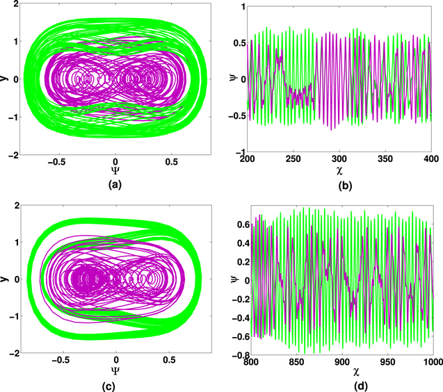
Figure 7. (a) Chaotic and quasiperiodic motions at initial conditions [0.08, 0] (purple) and [0.085, 0] (green); (b) corresponding time series. (c) Chaotic and quasiperiodic motions at initial conditions [0.089, 0.4] (purple) and [0.081, 0] (green), respectively; (d) corresponding time series for phase space f0 = 0.6, Ω = 3, and other parametric values the same as in figure 3.
Download figure:
Standard image High-resolution imageWe have presented time series plots depicting the existence of chaos in the system (15). To support our result, we use the most efficient method known as Lyapunov exponents. The sensitivity of chaotic motion to initial conditions is shown by positive values of the Lyapunov exponent. Here, the strength of the external force (f0) and its frequency (Ω) significantly change the dynamic motion of the system (15). Therefore, we plot the Lyapunov exponent against f0 and Ω in figures 8(a)–(b) and 8(c)–(d), respectively, with other parametric values the same as in figure 7. From figures 8(a)–(d), we observe that the system (15) preserves its conservative property (13). In figures 8(a)–(b) and 8(c)–(d), the positive values of Lyapunov exponent indicate the existence of chaotic behaviors, which are shown in figures 7(a) and (c), respectively. Here, in figure 8(a), we observe that f0 in the region (1, 1.2) depicts the existence of quasiperiodic attractors, while the region with f0 greater than 1.2 shows strong chaotic motion. In figure 8(b), the region with f0 less than 0.94 shows quasiperiodic motion and that with f0 greater than 0.94 shows chaotic motion. Similarly, in figure 8(c) at the initial condition (Ψ, y) = [0.08, 0] the regions Ω ∈ (0.43, 1.105) and (3.52, 3.74) depict the existence of quasiperiodic attractors, while the region Ω ∈ (1.27, 3.51) shows chaotic behavior. However, in figure 8(d) at the initial condition (Ψ, y) = [0.089, 0.4], the region with Ω greater than 0.175 depicts chaotic behavior. Hence, figures 8(a)–(d) show how f0 and Ω affect whether the Lyapunov exponents exhibit positive values for chaotic behavior or zero for quasiperiodic behavior.

Figure 8. Plots of Lyapunov exponents versus f0 in (a) and (b) for chaotic behaviors with parametric values the same as in the phase plots in figures 7(a) and (c), respectively. Plots of Lyapunov exponents versus Ω in (c) and (d) for chaotic behaviors with parametric values the same as in the phase plots in figures 7(a) and (c), respectively.
Download figure:
Standard image High-resolution image
5. Conclusions
The transmission of EAWs in electron–ion plasmas has been studied under the NLS equation. Supernonlinear periodic EAWs have been examined through phase plane plots along with nonlinear solitary and periodic waves. It has been shown that the nonextensive parameter q and v significantly affect both the nonlinear and supernonlinear EAWs waves. In addition, the multistability behavior of EAWs has been examined under the impact of an external perturbation force. For lower values of f0 and Ω, periodic and torus-like quasiperiodic patterns have been observed. However, for a significant impact of the external force, various patterns of chaos and quasiperiodic behaviors have been observed by changing the initial conditions. The study of nonlinear and supernonlinear EAWs with their multistability behavior in classical plasmas under the NLS equation has been reported for the first time. The results of the present work can be helpful in understanding different nonlinear electron-acoustic structures in the laboratory as well as in astrophysical plasma environments.