Abstract
Combined jumping and gliding locomotion, or 'jumpgliding', can be an efficient way for small robots or animals to travel over cluttered terrain. This paper presents functional requirements and models for a simple jumpglider which formalize the benefits and limitations of using aerodynamic surfaces to augment jumping ability. Analysis of the model gives insight into design choices and control strategies for higher performance and to accommodate special conditions such as a slippery launching surface. The model informs the design of a robotic platform that can perform repeated jumps using a carbon fiber spring and a pivoting wing. Experiments with two different versions of the platform agree with predictions from the model and demonstrate a significantly greater range, and lower cost-of-transport, than a comparable ballistic jumper.
Export citation and abstract BibTeX RIS

Content from this work may be used under the terms of the Creative Commons Attribution 3.0 licence. Any further distribution of this work must maintain attribution to the author(s) and the title of the work, journal citation and DOI.
1. Introduction
Jumping is an effective way for animals and robots to clear obstacles and scales favorably as size decreases and strength to weight ratio increases. An impressive array of jumping robots have been developed, providing insight into methods for efficiently storing potential energy and converting it into kinetic energy at a variety of scales [2–14].
In nature, vertebrates like the flying squirrel, flying fish, and flying snake use aerodynamic surfaces on their bodies to extend their jumping range, increasing their ability to avoid predators and negotiate terrain [15–17]. In robotics, a similar capability could decrease the cost of transport (CoT) for a jumping robot navigating around obstacles and over rough terrain for applications like exploration and search and rescue. Robotic platforms have also begun to include deployable surfaces [18–20] or fixed wings [20, 21] to increase range and control authority, and a simple model has been developed for jumping and gliding [20]. The ability to jumpglide could extend horizontal distance traveled for a given amount of stored energy, allow greater control over the details of trajectory, and create gentler landing conditions. However, care must be taken to ensure that the gains in performance offset the additional weight and drag associated with adding the ability to glide.
This paper examines the functional requirements for efficient jumpgliding. A candidate jumpgliding platform satisfying these requirements is presented and analyzed with both an analytical model and a detailed dynamic model to gain insight into the nuances of the proposed locomotion. Findings from the models are incorporated into a prototype capable of repeated autonomous operation. The predictions of the models are verified for controlled launches using the prototype presented here and an earlier half-scale prototype [1] that lacks the ability to compress its own launching spring.
2. Functional requirements for efficient jumpgliding
The CoT, a measure of locomotion efficiency, is defined as  , where E is the energy required by a mass (m) to travel a certain distance (d). The maximum possible CoT of a ballistic mass is fixed at 0.5, assuming flat ground and no energy recovery at landing. Jumpgliding offers a way to reduce the CoT of jumping robots. Conceptually, if an immediate transition to steady-state gliding occurred exactly at the apex of a 45° ballistic trajectory, one could achieve a CoT on flat ground of:
where  is the glide ratio, also defined as the ratio of horizontal to vertical velocities. Observed glide ratios range from 2 for the flying squirrel [15] to 50–70 for modern sailplanes. Thus, significant CoT reduction is expected from the combination of jumping and gliding. New functional requirements emerge for robots performing long jumps, as oppose to high jumps, and for jumpgliders seeking to reduce CoT. The identified requirements are as follows:
- (i)Prevent slip at takeoff. Long ballistic jumps require a coefficient of friction equal to one to maximize the range. This elevated value can be achieved with careful material selection for the foot or by taking advantage of surfaces asperities. Techniques which optimize performance at a higher jump angle would also be effective.
- (ii)Minimize the drag at takeoff. High takeoff speed is required to achieve significant jump height or distance. Studies of jumping insects demonstrate the importance of minimizing the ratio of drag to inertial forces for efficient jumping [22]. Minimizing this ratio is particularly challenging for jumpgliding as the wing adds significant surface area that is susceptible to creating increased drag.
- (iii)Perform an efficient transition from ballistic motion to gliding. Transition to gliding must be quick, timely and energy efficient. Losses during the transition will be amplified by their influence on the remaining glide.
- (iv)Gliding performance. Many parameters must be taken into consideration for optimal gliding performance, including wing sizing, aspect ratio (AR), angle of attack (AoA), etc. Many of these characteristics depend on the flight speed. Furthermore, if the velocity at the end of the ballistic phase was not oriented in the forward direction, redirection would be required, and would pose some efficiency and maneuverability challenges.
The proposed concept, illustrated in figure 1, uses a freely pivotable wing during the upward phase which attaches to the body at the apex to begin gliding. This concept minimizes the drag at takeoff and allows for a nearly ballistic upward phase. The pivotable wing also continuously aligns itself with the airflow throughout the upward phase. This self-aligning behavior brings the wing into gliding position at the apex, providing an immediate, energy efficient transition. At the apex, the remaining forward velocity allows the jumpglider to start gliding. Further analysis will demonstrate that the takeoff angle maximizing the distance traveled on flat ground is increased in comparison to a ballistic jumper, thus reducing the foot friction requirement at takeoff.
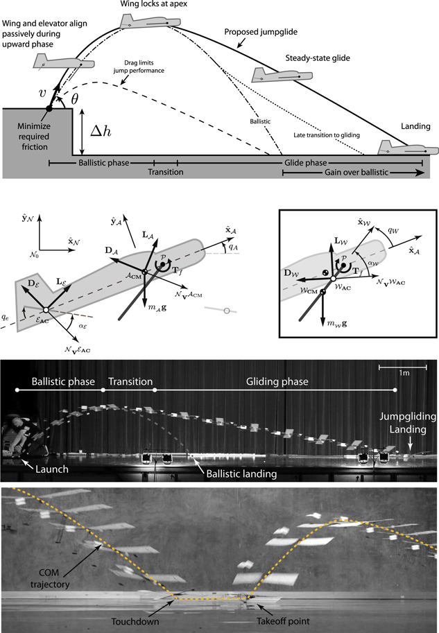
Figure 1. Top: functional requirements and proposed jumpgliding strategy as modeled in this paper. The dashed lines indicate trajectories representing failures in meeting one or more of the functional requirements. Center top: diagram of reference frames and forces on the plane body, wing, and elevator used in the detailed model. The left drawing highlights forces and moments on the body; the right drawing highlights forces and moments on the wing. The reaction forces at the wing pivot ( ) are not illustrated for simplicity. Reproduced with permission from [1]. Copyright 2013 IEEE. Center bottom: typical trajectory for the jump glider during model verification. The illustrated frames correspond to trajectory B in figure 6. Frames are spaced by 83 ms during the ballistic phase and by 166 ms during the glide phase. Glide ratio is 6:1. Bottom: typical trajectory for the jumpglider landing, loading the spring and jumping away from the camera.
Download figure:
Standard image High-resolution imageThe remaining sections of this paper develop models to analyze the performance achievable by this jumpgliding concept. These models are also used to understand the design tradeoffs and guide the design of a functional prototype demonstrating reduced CoT in comparison to ballistic jumpers.
3. An analytic model for design
As discussed in section 2, the basic idea of jumpgliding suggests a possible reduction in CoT as compared to a conventional jumping robot. To formalize this insight, we develop an analytic model to capture the essential behavior of an ideal jumpglide. This model examines the theoretical upper bound of the basic jumpgliding strategy illustrated in figure 1 and is designed to answer the following questions:
- (i)What is the maximum jump gliding distance?
- (ii)What is the optimum combination of jump angle, initial velocity and starting jump height?
- (iii)What are the most important design parameters?
- (iv)How does it compare to a wingless ballistic jumper?
The analytic model divides the maneuver into three phases: an initial ballistic phase from launch to apex, a transition phase between apex conditions and conditions required for steady state gliding, and a final gliding phase. The analysis differs from that presented in [20] both in the basic approach (pivoting versus fixed wing) and especially in the analysis of the transition phase, discussed below. The following sections describe this model in terms of the horizontal ( ) and vertical (
 ) distances predicted for each phase.
3.1. Ballistic phase
The first phase assumes a ballistic trajectory during which lift and drag are negligible. Under these conditions the distances traveled during the ballistic phase of the jumpglide are simply:
where  and
and  are respectively the horizontal and vertical distances traveled by the jumpglider during the ballistic phase,
  is the initial velocity of the jumpglider and θ is the jump angle.
3.2. Transition
After the jumpglider passes the apex of the jump, it continues along an approximately ballistic trajectory until the vertical velocity is sufficient for gliding to commence. Including this transition phase between ascent and glide affords a better estimate of performance since traveled distance would be underestimated if gliding were started immediately at the apex. In contrast to [20], which assumes an immediate drop in height to achieve a predetermined glide velocity and slope, the transition phase presented here allows for a ballistic transition to a steady-state glide. The speed and slope of this glide vary based on initial conditions and jumpglider design. The required vertical gliding velocity depends on the forward velocity imparted by the jump and on the airplane mass ( ), wing area (A) and zero-lift drag coefficient (
 ). To solve for the vertical velocity at which the transition occurs, one can use the lift to drag ratio,
  , for flat plates at small angles of attack:

This equation is difficult to solve for  as it implies a fifth order equation in
  . Furthermore, it is limited to glide regimes where the forward velocity is high compared to the vertical velocity—a condition that requires a higher
  than is typically achieved in jumpgliding at this scale.
A more suitable approach, therefore, is a linear approximation between a free fall glide ( ) and gliding at the maximum
  . The maximum
  and the velocity at which it occurs can be found by equating both terms of the denominator in equation (3):
Knowing that  is equal to zero at zero forward velocity and assuming that the forward velocity
  at maximum
  is approximately equal to
  , it is possible to linearly approximate the relationship between
  and the forward velocity, subject to the condition that
  :
:

The new constant parameter  is defined as:

Assuming a ballistic trajectory, the end of the transition phase is obtained by solving for the displacement needed to reach the vertical velocity required to start gliding (i.e., vyG ):
3.3. Gliding
Once the vertical velocity required for gliding is reached, the distance traveled during the glide phase is calculated by multiplying the glide ratio ( ) with the altitude above ground level of the jumpglider at the start of this phase:
where  is the elevation lost between the start and finish point.
3.4. Results
With each phase defined, the total distance traveled is calculated as:
All terms of this equation are positive under typical conditions since  is negative. For even a small
  , the second term is small in comparison to the others. Equation (9) can be thought of as a template for control strategy and as a guide for the designer in specifiying the best possible performance. It will generally overestimate the distance traveled as it neglects effects like negative lift on the elevator, body drag during the upward phase, etc. The comparison between this analytical model and the full dynamic model (developed below in section 4) is described in [1] and illustrated in figure 2.
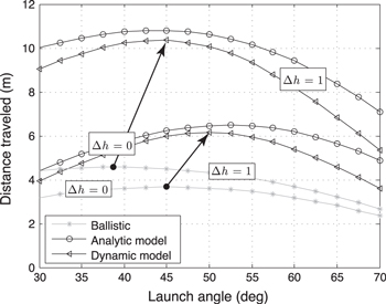
Figure 2. Jumpgliding increases both the distance traveled with respect to a ballistic jumper and the jump angle maximizing the range, as indicated by the arrows drawn from the ballistic peaks to the jumpgliding peaks. As for a ballistic projectile, the optimum jump angle for jumpgliding decreases with increasing  . The analytic model slightly over-predicts distance traveled compared to the full dynamic model due to body drag, elevator effects and the linear approximation of
  vs forward speed. Results are for the jumpglider presented in [1] (
 ,
,  ,
,  ,
,  ,
,  and
and  ).
).
Download figure:
Standard image High-resolution imageEquation (9) can be used to answer questions (i) and (ii) posed at the beginning of this section. Although it is non linear in θ it reveals clearly how the optimal jump angle varies with  and
and  . For a fixed airplane design (i.e. fixed
  ) the first term is largest for a θ of 45° (to maximize
  ), the second term is always small, the third term favors a θ of around 54° (
 ) and the last term favors a horizontal launch (
 ). The importance of these terms varies given the launch conditions: the third term is more important at higher launch speeds while the last term is more influential with larger changes in elevation. The optimal jump angle for a flat surface is 52° but reduces to 44° when the drop height increases to 1 m, as illustrated in figure 2.
In answer to question (iii), one can analyze the parameter  (equation 6). As the magnitude of this parameter decreases, the distance traveled will increase. This parameter can be reduced by changing the design of the jumpglider to decrease the mass to lifting surface area ratio and the parasitic drag coefficient. This is non-trivial as the mass and parasitic drag coefficient both tend to increase with wing area. Finding the optimal wing size is left as future work but could be done with multi-disciplinary optimization techniques.
To answer question (iv), it is useful to define the distance traveled by a ballistic jumper ( ). This distance, for a jumpglider of mass
  launched with an initial velocity
  and an initial height of
  , can be expressed as:
As expected, this equation simplifies when  and the optimal jump angle becomes
  . One can then use the relations in (9) and (10) to calculate the distance gained
  by adding a wing:

Note that each optimization must be done independently as the optimum jump angle (θ) is different for ballistic and jumpgliding robots. To determine when the gliding phase overcomes the penalty of adding the mass of the wing, one can relate the jump energy (E) to the takeoff speed of a ballistic jumper of mass  and to that of a jumpglider of mass
  :
:

Figure 3 illustrates the influence of the wing mass with respect to body mass ( ) and jump energy (E) on the distance gained (
 ) for various wing areas (A) and initial jump heights (
 ). The analytical model predicts, as shown by the white square in figure 3 top-right inset, that the prototype described in this paper can cover a distance about 30% greater than a 52.5 g ballistic jumper, even with a 15 g wing. Higher jump energy or better wing-to-body mass ratio would increase the traveled distance. As expected, a smaller wing size (top-left inset) would produce less impressive gains for a more limited range of
  . As pointed out in [21] and illustrated in the left and right lower inset in figure 3, jumpgliding shines when some initial height is available. For both wing sizes, lighter wings (i.e. low
  ) increase the traveled distance.
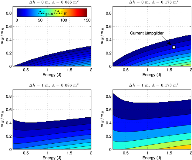
Figure 3. Favorability of adding wings to enable jumpgliding for different manufacturing constraints, wing areas, and initial conditions (calculated for  and
and  ). The energy available for jumping (E) and the ratio of the mass of the wing to the mass of the body (
 ) depend on the materials and processes used for fabricating the wing and the spring. Based on these conditions, the predicted gain for conversion from jumping to jumpgliding is computed (
 in percent) and displayed as a color gradient. White represents negative gain. Gain improves with increased wing area, increased jump height, decreased
  and increased E. The white square in the top-right figure represents the characteristics of the glider described in this paper. The predicted 28% increase corresponds to experimental results presented in figure 6.
Download figure:
Standard image High-resolution image4. Planar simulation of full jumpgliding dynamics
While the analytic model presented in section 3 provides fundamental insight into the design of a jumpglider and suggests the upper bound of performance improvement, a higher fidelity model is desirable to capture some of the important and inescapable non-idealities inherent in a specific implementation. To address this need, a detailed dynamic model was developed to simulate the jumpgliding design shown in figure 5. The complete behavior is complex, posing a hybrid discrete-continuous dynamics problem with aerodynamic and ground reaction forces. However, by assuming a straight jump which creates negligible roll and yaw velocities, a planar aerodynamic model appropriately captures the evolution of the aerial behavior. The planar simplification allows us to select a specific approach based on a modified dynamic model of airplane flight. In this model, rigidly attached wings are replaced with wings attached to the plane by a pin joint. This allows them to rotate freely during ascent to minimize losses due to aerodynamic forces. The wings are then locked in place at the top of the trajectory to generate lift during the descent. The basic approach is illustrated in figure 1.
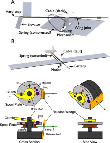
Figure 5. Implementation details for this jumpglider. Top: CAD rendering of the prototype before launch (A) and during the glide (B). The loading and release mechanism compresses the spring for launch using power from the battery. The wing and the elevator are free to rotate during ascent; both are pulled against hard stops as the descent begins, locking them in place for gliding. Bottom: diagram of the autonomous loading and release mechanism. See text for description.
Download figure:
Standard image High-resolution imageOur dynamic model consists of two rigid bodies: the wing, with associated reference frame  , and the airframe, with associated reference frame
  . Frame
  is rotated with respect to the Newtonian reference frame
  by an angle
  (pitch) around the unit vector
  , and
, and  is rotated with respect to
  by an angle
  around
  . The positions of the center of mass (CM) of the airframe,
  , and the CM of the wing,
  , can then be represented as:


where  is the distance from
  to
to  , the wing pivot point, along
  and
and  is the distance from
  to
to  along
along  .
.
The modeled forces include gravity on the airframe and wing, friction at the wing pivot point, and lift and drag on the wing, the elevator and the body. These forces are illustrated in figure 1.
For the Reynolds numbers that apply to the jumpgliders presented in this paper (i.e., 30 000–50 000), a flat plate model is appropriate to represent the lift L and drag D on the wing and elevator [23, 24]:


where ρ is the air density and  is the velocity of the aerodynamic center (AC) in
  , and
, and  and
and  are the area and the AoA of the aerodynamic surface i, respectively. In still air, α represents the angle between the velocity of the AC and the vector from the trailing edge to the leading edge of the aerodynamic surface. Drag opposes the velocity of the AC, lift is perpendicular to it, and both forces are applied at the quarter cord (measured from the leading edge). An additional parasitic drag force on the body
  is applied at the the airplane's CM.
Pivot friction is simulated as viscous damping and applies a torque of  on the wing. Viscous damping was chosen because of its simplicity in numerical simulation. The wing pivots at a roughly constant angular velocity through the ballistic phase for jump angles of 30–65°, so the effects of a viscous term are similar to those of Coulomb friction; furthermore, the frictional torque is small compared to other terms.
At the apex of a jump, the wing locks into place to begin gliding, which is simulated by a stiff torsional spring and damper enabled for  . The spring-powered launch is approximated by specifying the velocity of the airplane at take-off using the observed initial conditions.
The acceleration of the CM, angular velocity and angular acceleration of each body i are denoted as  ,
,  and
and  , respectively. Using a D'Alembert approach, the sums of forces and moments on the system are equated to the sums of inertial terms, referred to as effective forces and effective moments [25]. Analysis of the forces and moments on the system and the moments on the wing results in three vector equations:


Equation (17) is dotted with  and
and  , and equations (18) and (19) are dotted with
  to produce four scalar equations which are then solved for
  ,
,  ,
,  and
and  . In the present case the solutions were obtained using Motion GenesisTM [26] and solved numerically in MatlabTM. These simulations provide insight into the behavior of the jumpglider.
4.1. Influence of aerodynamic forces during ascent phase
As pointed out in section 2, minimizing drag during takeoff is critical. Ideally, the freely pivotable wing perfectly aligns itself with the airflow, but in practice friction at the wing pivot joint can cause the AoA (α) to be non-zero during ascent, creating additional lift and drag. For a small AoA, lift dominates because it grows in proportion to α while drag is proportional to  . Furthermore, in still air, lift is a conservative force because it is orthogonal to the instantaneous direction of motion, and so is predicted to change the shape of the trajectory without reducing the energy available to the glider. Thus, small amounts of lift caused by friction at the pivot should change the trajectory of the airplane by reducing the forward velocity and increasing the height of the apex, similar to the effect of a slightly steeper initial launch angle.
To further examine the interplay of variations in launch angle and lift during ascent, simulations were performed for different combinations of launch angles and friction at the wing pivot, the results of which are illustrated in figure 4. For a frictionless pivot, the jump angle which leads to the maximum distance traveled is around 52°. With increasing friction, the lift contribution causes the optimum jump angle to decrease, but the maximum distance traveled remains nearly constant until the friction is more than four times greater than the value measured for the jumpglider discussed in [1].
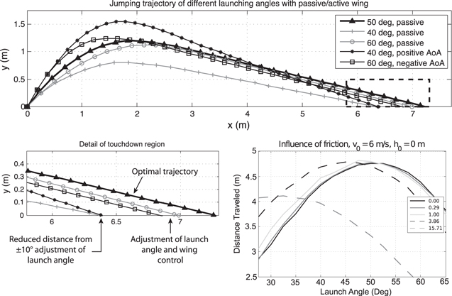
Figure 4. Top: influence of lift during the ascending phase for simulated launches. The center trajectory illustrates the flight trajectory of a passive wing glider with near optimal jump angle ( ). The two outermost trajectories represent deviations from that ideal launch angle by plus or minus 10° for the same passive wing glider. The remaining two trajectories indicate attempts to recover from non-ideal launch conditions by using lift during ascent. To create this lift, a controller applies a torque to the wing proportional to its angular velocity. For the two cases illustrated, this results in an AoA of the wing that is almost constant through the upward phase at approximately plus or minus
  . In both cases, either with positive lift at 40° or negative lift at 60°, the range is extended. Bottom left: greater detail for effects of lift on range, indicating initial performance loss for non-ideal jump angles and performance recovery from using lift during the ascent. Bottom right: for small amounts of pivot friction, the maximum distance traveled is not affected but the launch angle (θ in figure 1) should be reduced to compensate for the lift created. The different curves correspond to varying amounts of effective damping coefficients normalized relative to the performance of the initial prototype.
Download figure:
Standard image High-resolution imageThe insensitivity to small amounts of pivot friction justifies the choice of a passive solution for varying wing angle, as adopted in the prototype presented here, and in a smaller and simpler prototype in [1]. It also suggests the more general result that small amounts of lift can be used to change trajectory without sacrificing significant energy in increased drag. One application of this result would be to extend the range of take-off angles which lead to good gliding conditions. By using the wing of the jumpglider as a control surface during ascent, optimal peak heights and forward velocities can be achieved from a range of jump angles. This is particularly important considering that a jump at 40° requires a ground coefficient of friction of at least 1.19 while a jump at 60° requires a more reasonable coefficient of 0.57. As figure 4 illustrates, both the 40° and the 60° launches reduce the total traveled distance by about one meter (13%) when compared to a 50° launch. By using a negative AoA during the ascent the lost distance for a jump at 60° is reduced from 13% to 6%. Conversely, one can use a positive AoA during a launch angle of 40° to reduce the lost distance to 3% of the distance traveled when launched at 50°.
These strategies lose their effectiveness once the lift demanded requires a significant AoA. If α becomes large, drag will subtract non-negligible energy during ascent, resulting in poor glide conditions and decreased range.
5. Implementation
The claims made by these models can be tested on robotic platforms. An earlier prototype had a mass of 30 g, a wingspan of 70 cm, a cord of 11.5 cm and flew at around 4  with a glide ratio around 2.6 [1]. It also used a 1.0 g Micro 9-S-4CH receiver and a 2.5 g Blue Arrow Servo to manually control the elevator. The jumpglider presented in this paper is larger than the prototype presented in [1] to accommodate the autonomous loading and release mechanism.
5.1. Jumpglider and wing sizing
The jumpgliders must achieve a high glide ratio (i.e., high  ) at speeds which can be created by a reasonable jumping mechanism. It has been shown that, for wings at Reynolds number between 30,000 and 50,000, an
  of six provides similar performance to a wing of higher AR without the practical disadvantages of a very long and slender wing [27, 28]. At these Reynolds numbers and at an
  = 6, a rectangular planform (wing shape) also outperforms an elliptical planform. The same studies also show that a rectangular wing with
  = 6 can be expected to have a
  around 8–12, peaking at 3–4
 of AoA which corresponds to a lift coefficient (
 ) of 0.4. Although a 5% cambered airfoil provides better performance, a flat wing was used in the prototype for ease of manufacturing and damage repair.
The jumpglider presented in this paper has a wingspan of 1.12 m, a wing cord of 15 cm and a mass of  . A glide ratio (
 ) of six was reached at a flight speed of around 4.5 m s−1. This corresponds to a Reynolds number of about 50,000 and lift coefficient of 0.35, as expected from [27, 28]. The CM of the jumpglider is located just ahead of the wing's aerodynamic center (i.e. the quarter cord) and 35 cm ahead of the elevator's aerodynamic center. The elevator measures 14 cm by 8 cm. This arrangement is designed to produce longitudinal stability during gliding. The launch spring connects to the jumpglider via a pivot near the CM to create minimal angular acceleration over a range of jump angles.
The wing is made using 1 mm thick Pro-formanceTM foam and a leading edge carbon fiber spar for a total mass of 15 g. The previous jumpglider used a teflon bushing to let the wing freely pivot around the body. To reduce friction to a minimum, this new jumpglider attaches the wing to the body with a thin plastic flexure designed for minimal stiffness throughout the typical range of motion for the wing. The wing is locked into place for gliding at the apex of the trajectory through a simple hard stop. The body is built out of carbon fiber rod with laminated balsa wood and fiberglass FRP sheet structural elements. The jumpglider also carries a 110 mAh single-cell LiPo battery (enough for hundreds of jumps) and a 1000:1 micro metal gearmotor used to power the autonomous loading and release mechanism for the spring. The elevator is rotationally coupled to the wing by means of a string, which allows the elevator to approximately align with airflow during ascent (minimizing drag) and then be pulled against a hard stop to maintain the appropriate trim angle for gliding.
5.2. Spring design
The jumping mechanism design is primarily driven by the mass of the foot, the force profile on the ground and the energy density of the spring. Since the foot remains stationary until the end of the decompression phase, the mass of the foot should be minimized to avoid dissipating excessive kinetic energy [3]. The profile of the ground reaction force should be carefully chosen; the triangular force profile of a conventional spring can cause premature lift-off and high initial accelerations that excite various structural modes. Other alternatives include a geared power transmission system [2, 3] or a bow spring, which can create a nearly constant force profile. The advantages of a carbon fiber bow spring for jumping are discussed in [7]. Although elastomers can give higher specific energy, a carbon fiber bow spring still provides a favorable energy storage density [29] and a low loss modulus, and does not deteriorate as quickly as rubber.
The bent spring is an elastica that can be approximated as a set of rigid rods serially connected by torsional springs with stiffness  , where
  is the second moment of area and
  is the discretization length of each segment, as described in [30]. To find angular displacements,
  , when the tips are compressed to a distance
  apart, it suffices to minimize the potential energy:
This can be solved using Lagrange multipliers. Given angular displacements, the spring energy, tip forces, maximum bending moment and maximum stress are easily calculable.
For a 70 g jumpglider, 1.4 J is required to jump, at an angle of 45 , to a forward velocity of 4.5 m s−1 and a height of 1 m. Equation (20) suggests that the spring can store this amount of energy, and even more, with two unidirectional carbon fiber composite beams 32 cm long, 8 mm wide and 0.89 mm thick. The Young's modulus of the composite was measured as 120 GPa. When the distance between the tips of the spring is compressed to 9.4 cm the stored energy is 3.0 J. The maximum stress is 1.0 GPa (50% of the ultimate strength of the unidirectional carbon fiber). With a density of 1550 kg m−3, the carbon spring mass is 7.1 g. With the additional support structure, the manufactured spring weighs 9.9 g. Force-displacement data were collected for the spring and numerically integrated to show an energy storage of 2.55 J. Such variations from the model are expected due to its high sensitivity to minor variations in beam thickness and the fiber volume ratio.
Spring size could be reduced for equivalent energy storage by reducing length and increasing thickness and curvature, but this would also result in a higher peak force which might exceed the limits of the plane frame or the loading mechanism and which is more likely to induce undesired vibrational modes. Comparatively, the lighter prototype described in [1] uses a smaller (1.2 g) spring to store 0.53 J.
5.3. Autonomous loading and release mechanism
To enable autonomous operation, the carbon spring must be loaded and freely released repeatedly. In the presented solution, a motor winds a spool with an engaged clutch to tension a string that deflects the launch spring. Once fully deflected, a wedge disengages the clutch, and the spool freely unwinds.
The mechanism consists of a release wedge used as a trigger along with two other elements attached to a motor output shaft: a spool plate which is passively free to rotate and a clutch which can pivot about a pin that locks it to the motor shaft, as illustrated in figure 5. The spool plate contains five NdFeB magnets embedded into the face adjacent to the clutch, and the clutch contains one magnet along the same interface. The polarity of the magnets are chosen such that one of the spool plate magnets attracts the clutch magnet while the other four repel it. A stop is attached to the spool plate near the attractive magnet. When the angular velocity of the spool plate is low with respect to the clutch, the clutch is pulled toward the spool plate by the attractive magnet and caught by the stop. When the stop catches the clutch, a mechanical connection is formed between the spool plate and the rotation of the motor shaft, allowing winding of the string. However, when the angular velocity of the spool is high, the other four magnets combine to create a net repulsive effect which prevents the clutch from engaging.
During operation, the motor turns slowly, the clutch engages, and the string winds on the spool to tension the spring. When the spring reaches a set deflection, a release knot translates the release wedge into a position which disengages the clutch on its following pass. The spool then unwinds rapidly on its ball bearings, during which time the clutch is repelled by the average magnetic force. When the spool comes to rest at the end of the spring extension, the cycle repeats.
The advantages of this design include its low weight, the low control overhead necessary for its operation, and the minimal resistance created during spring extension. The motor chosen weighs 11 g, and the mechanism adds 2 g.
6. Results
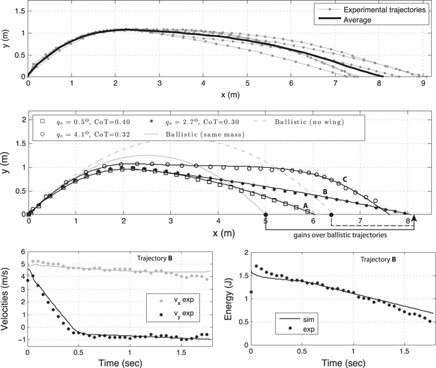
The airplane was launched with various initial conditions and was recorded at 60 and 400 fps using a high-speed camera. After calibrating the camera to compensate for distortion, the CM position is tracked in each frame. The resulting position is filtered by a seven point moving average filter. The width of the filter is chosen to reduce the noise before differentiating the signal to calculate the velocity without modifying the trajectory. The energy level is calculated by summing potential and kinetic energies. Results are illustrated in figure 6.
Figure 6. Top: six consecutive jumpgliding trajectories are plotted in gray, with the thick black line representing the average position. The average distance traveled is 8.1 m, with a standard deviation of 0.8 m. The CoT for each flight ranges from 0.29 to 0.36. Center: comparison of three experimental flights (discrete marker) with their corresponding trajectories computed with the dynamic model (solid black lines). These three jumpgliding trajectories represent a range of jumpgliding behaviors: short jumpglide created by diving (A), steady glide slope (B) and stall-like behavior (C). These behaviors are matched in the model by adjusting  , the elevator angle used during the glide phase. Initial energy is 1.65 J, 1.66 J and 1.97 J for trajectories A, B and C respectively (this value is proportional to v from figure 1). The position was normalized by the energy of B to enable better visual comparison of the CoT of each trajectory. The two drag-free ballistic trajectories (grey) are computed for a 67.5 g and a 52.5 g (no wing) projectile launched at 45
 with the takeoff energy of B. Bottom: comparison of experimental and simulated velocities (left) and energy level (right) during jump gliding for trajectory B. The transition from ballistic motion to gliding happens around 0.5 s.
Download figure:
Standard image High-resolution image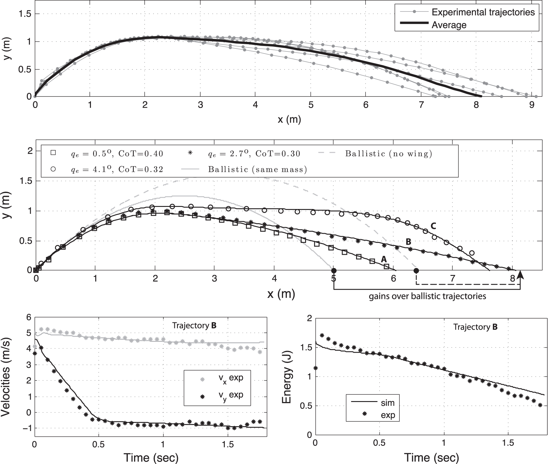
To characterize the aerodynamic performance and repeatability of the jumpglider, the plane was launched by an external launcher to specify the launch conditions. Six consecutive runs are plotted in figure 6. The spring system was replaced with equivalent dead weight.
For experiments used to verify the model, the launch spring is manually loaded by pulling on a Spectra line, which is then cut by a heated nichrome wire for takeoff. This ensures precise control of launch conditions for repeatability. The wind and release mechanism is left in place to maintain the correct mass properties. The model parameters used in these figures are: wing area of 0.17 m2, elevator area of 0.011 m2, body area of 3
  m2, zero joint friction, body mass of 52.5 g, wing mass of 15 g, body inertia around its CM of 6.0
  kg m2 and wing inertia around its CM of 3
  kg m2. The zero-lift coefficient (
 ) was measured by comparing the initial part of the experimental trajectory, where the wing and elevator freely rotate, to the dynamic model, and finding the value which produced the measured reduction in energy during the ballistic phase. A
  of 0.015 was measured for the three trajectories illustrated in figure 6. It should be noted that, while the model assumes a continuous wing, the actual wing has a slot removed near the center to accommodate the carbon spring during launch. This and other aerodynamic non-idealities contribute to the magnitude of
  .
.
After measuring the initial velocities experimentally, the elevator angle during gliding ( ) was adjusted in the dynamic model to fit the three experimental trajectories illustrated in figure 6 (center). The identified elevator commands varied from 0.5 to 4.1° and show good fit for both the the ballistic and glide phases. The velocities and energy of the system, illustrated for trajectory B in figure 6, also show good agreement with the model. The first phase (
 ) is essentially ballistic, with slow reduction in energy due to body drag. The second phase shows almost constant velocity and a higher rate of energy reduction due to drag on the wings, consistent with a steady glide.
In all the cases illustrated, the jumpglider does not go as high as a drag-free ballistic trajectory with a 45 launch angle. Nonetheless, it still travels further than the drag-free ballistic trajectory. In the case of trajectory B, this gain reaches 66% as detailed in table 1. The distance is also longer than a drag-free ballistic trajectory with the same initial energy but without the mass of the wing (25% in case of trajectory B). To the knowledge of the authors, this is the first time that such performance is demonstrated. Further improvements are possible since the wing is quite heavy in this prototype (15 g) and the launch angle shown here is a little shallower than the ideal angle predicted by the model. This launch angle was selected for analysis based on ease of extracting accurate data from the recording. Launches in the field with different launch angles were observed to reach distances 1.5 m longer than depicted in figure 6.
Table 1. Comparison between jumpgliding and ballistic trajectories with and without the mass of the wing. The jumpglider presented in this paper travels further than an equivalent ballistic jumping robot using the same level of energy, even when considering the increase in mass due to the wing. CoT is calculated relative to the energy measured at the beginning of the jump, and is reduced from 0.5 to 0.3 by the combination of jumping and gliding.
| Jumpglider | Jumpglider [1] | Current jumpglider (trajectory B) | Ballistic |
|---|---|---|---|
| Mass body (g) | 23.8 | 52.5 | m |
| Mass wing (g) | 6.2 | 17.5 | — |
| Energy at takeoff (J) | 0.63 | 1.66 | E |
| Jumpgliding on flat ground (m) | 5.01 | 8.06 | — |
| Ballistic with same mass and energy (m) | 4.28 | 4.83 |

|
| Ballistic with same energy but no wing mass (m) | 5.40 | 6.45 | — |
| Cost of transport | 0.44 | 0.30 | 0.5 |
Of these trajectories, flight B has the lowest CoT, at 0.3, followed closely by flight C at 0.32. Increasing pitch to maintain lift as the velocity is reduced, as in flight C, results in less excess energy dissipated at touchdown. It is still unclear at this point if longer distances could be achieved with such a technique. Table 1 also compares these results to the smaller prototype detailed in [1].
Although the experimental characterization of the spring suggests an energy storage of  , the measured kinetic energy of the plane shortly after launch varies between 1.6–2 J. This loss can partially be explained by the geometry of the spring. In transitioning from a tensioned U-shape to a straight beam, the middle portion of the spring acquires significant kinetic energy in the direction perpendicular to the jump angle. This is then lost in vibrational modes and angular velocity of the spring. This loss is estimated from observation of the amplitude of oscillation to be
  and could be minimized by reducing the mass of the spring. Other losses result from material damping, vibrations in the aircraft frame and from slip at the foot.
The autonomous loading and release mechanism was tested by allowing the final prototype to launch itself multiple times sequentially as depicted in the time-lapse image in figure 1 and in the supplementary video (available at stacks.iop.org/BB/9/025009/mmedia). For the slippery surface navigated in this image, a steeper than ideal jump angle was necessary to avoid excessive foot slip.
7. Conclusions
This paper presents an autonomous jumping robot capable of repeated jumpglides. The addition of gliding offers many advantages over traditional jumping robots. In particular, additional aerodynamical control over trajectory can enable a steeper jumpgliding takeoff angle which reduces ground friction requirements and allows jumps on a variety of surfaces without sacrificing significant distance. Furthermore, the 6:1 glide ratio of the jumpglider presented in this work increases the traveled distance relative to a ballistic jumper and reduces the CoT accordingly. To gain more insight into the influence of the design parameters on the performance, a simplified analytical model was developed. This simple model shows that the reduction in ballistic distance caused by the added mass of the wing can be compensated for by gliding, and that even small and heavy wings can be beneficial for jumps from elevated starting heights. A first multi-body hybrid dynamic model including aerodynamic effects was also developed to predict the behavior of the jumpgliders and possible control strategies with higher fidelity. The analytic model predicts results similar to those predicted by the dynamic model, and the dynamic model was verified against experiments involving two prototypes of different size.
Future work includes adding greater control during the airborne phases and using more rigorous multi-disciplinary optimization to size all components simultaneously. Reduction in drag, addition of airfoil camber and reduction in wing and spring mass would provide immediate improvements. More generally, in light of these findings, it would be interesting to reexamine how animals use their wings and when they choose to jumpglide. Observation of animals might also offer insight into different jumpglider designs. Indeed, most animals do not simply pivot their wings to reduce drag on ascent but rather fold their wings against their bodies during that phase. Such designs should be less sensitive to gusts during the upward phase of the jump and may offer additional, unexplored benefits.
Acknowledgments
We thank Matt Estrada, Hao Jiang and other members of the Biomimetics and Dextrous Manipulation Laboratory for their advice and support throughout the project. Support for this work was provided by NSF IIS-1161679 and ARL MAST MCE 14-4. The dynamic modeling for this paper was done using MotionGenesis software. E Hawkes is supported by an NSF Graduate Fellowship.