


Abstract
Climate variability and extremes are expected to increase due to climate change; this may have significant negative impacts for agricultural production. Previous work has primarily focused on the impact of mean growing season temperature and precipitation on rainfed crop yields with little work on irrigated crop yields or climate extremes and their timing. County-level crop yields and daily precipitation and temperature data are pooled to quantify the impact of climate variability and extremes on four major staple crops in the United States. Conditional density plots are used to graphically explore the relationship between climate extremes and crop yields, thereby avoiding assumptions about linearity or underlying probability distributions. Non-linear and threshold-type relationships exist between yields and both precipitation and temperature climate indices; irrigation significantly reduces the impact of all climate indices. In some cases, this occurs by shifting the threshold, such that a more extreme weather event is necessary to negatively impact yields. In other cases, irrigation essentially decouples the crop yields from climate. This work demonstrates that irrigation may be a beneficial adaptation mechanism to changes in climate extremes in coming decades.
Export citation and abstract BibTeX RIS

Content from this work may be used under the terms of the Creative Commons Attribution 3.0 licence. Any further distribution of this work must maintain attribution to the author(s) and the title of the work, journal citation and DOI.
1. Introduction
In the coming decades, we are presented with the challenge of feeding a growing population in the face of climate change—two potentially major stressors to the global food system. Some studies have predicted that an expansion in cropped area will be necessary in order to increase production to meet growing food needs, but many of these regions may be in marginal regions and require irrigation (Bruinsma 2009). From an agricultural perspective, irrigation water use is a positive phenomenon, leading to increased yields and more stable production, but little research has focused on how it buffers against a range of climate extremes to better inform predictions of climate change impacts in the agricultural sector.
There is a significant body of literature linking climate conditions and crop yields, particularly in the context of the potential impacts of climate change on agricultural productivity. Using crop models and future climate scenarios from global circulation models, a decrease in agricultural production is predicted, although uncertainty exists in the crop responses to certain conditions, including crop response to high temperatures (Rosenzweig et al 2014). Regional studies indicate a projected decrease in the mean yield of eight major crops grown in Africa and South Asia by 2050 (Knox et al 2012). Using historical data to understand crop yield responses to climate conditions, it was found that both temperature and precipitation are key factors for predicting yields (Lobell and Burke 2008), with growing season precipitation and temperature explaining over 30% of year-to-year yield variations (Lobell and Field 2007). Statistical models have demonstrated that temperature trends have caused decreased maize and wheat production globally (Lobell et al 2011). A recent meta-analysis has shown that decreases in global wheat, rice, and maize production will occur due to climate change without adaptation (Challinor et al 2014). These studies are useful for anticipating the effects of climate change on crop yields; however large spread exists across the modeled crop yield responses, as has been shown for wheat (Asseng et al 2013), leaving open questions about how to adapt to mean growing season changes over the coming decades.
In addition to growing season mean temperature and precipitation affecting yields, studies have suggested increasing climate extremes and variability will affect crop yield and production (Rosenzweig et al 2001, Porter and Semenov 2005). Despite this, few studies specifically analyze the impact of extremes, either with historical data or in model projections. For example, crop model simulations that use GCM output (Rosenzweig et al 2014) contain climate extremes that can affect the yields but the analysis is done as a yield response to mean temperature change. This is unsurprising: it is challenging to aggregate data across a variety of growing regions, and most climate studies look at response as a sensitivity function to degree temperature change (or precipitation change). However, extremes are equally important to consider. For example, maize yields in the United States appear to be increasingly sensitive to drought, despite the yield increases over the past decades (Lobell et al 2014). Extreme heat (greater than 34 °C) negatively impacts wheat yields in India (Lobell et al 2012). Losses of maize yields and spring wheat yields are projected to double by the 2080s due to increases in heat stress at anthesis (Deryng et al 2014). Observed data collected through a controlled environmental experiment in Germany has confirmed the impacts of heat stress on rye and wheat yield decline (Siebert et al 2014). Higher night temperature extremes (32 °C) can impact rice yields (Mohammed and Tarpley 2009). Rainfall variability is also crucial for interannual yield variability at aggregated level and at the plot level. A drought index was found to be associated with several winter and spring sown crop yields at county level in Czech Republic (Hlavinka et al 2009). All of these studies not only point to the importance of better understanding of the impact of climate extremes on yields across growing regions but also to the challenges to studying climate extreme impacts.
Irrigation allows crop cultivation in climates that do not receive sufficient rainfall and buffers stress due to climate variability and extremes on agricultural production. Irrigated agriculture provides a significant contribution to global grain production: irrigated lands are 17% of total cropped land, yet they provide 40% of global cereals (Cai 1999, Rosegrant et al 2002, Siebert and Döll 2010). Even in regions with sufficient seasonal rainfall, irrigated yields can surpass rainfed yields (Grassini et al 2009), likely due to sub-seasonal variability in rainfall. Pearson's correlation coefficients calculated for yields and climate variables, such as mean, maximum, and minimum temperatures, precipitation, and radiation, revealed varying correlation strengths depending on the climate index and timing of extreme. For example, rainfed maize is more sensitive than irrigated maize to maximum temperature earlier in its growing season (pre-silking); later in the growing season (post-silking), rainfed and irrigated maize shows the same sensitivity to maximum temperatures (Grassini et al 2009). Many of these studies use correlation coefficients to establish a relationship between climate and yields. However, correlation coefficients assume a relationship exists throughout the distribution of the data; for extreme climate indices this may not be the case. Quantifying the impact of climate extremes on rainfed versus irrigated agriculture will allow for better climate adaptation planning in the agricultural sector.
To fill the gap in our understanding of the impact of extremes on crop yields, both irrigated and rainfed, this study uses historical, county-level data over the United States. By pooling each county and year together, we are able to overcome the typical small sample size that plagues analysis of extremes. By using novel graphical techniques, we are able to establish which extremes negatively impact crop yields with no a priori assumptions about the form of relationship (e.g. linear, quadratic, etc). Utilizing a USDA dataset that includes both irrigated and rainfed yields for a subset of US counties, the analysis presented here is able to evaluate how much irrigation can mitigate against the effects of climate variability and extremes, thereby providing a more nuanced view of agricultural water use which can further help in assessment of agriculture, irrigation, and water resources in the coming decades.
This study has several objectives. First, we introduce a graphical technique useful for establishing relationships between two variables in large datasets. The technique allows for a representation of the probabilistic response of crop yield to climate indices. Second, we use this technique to evaluate the effect of climate (both seasonal means and extremes) on crop yields at the county-level in the US. This provides an analysis of data at larger spatial scales to complement the many field-scale studies on this topic. Third, using a subset of the counties for which data is available, we quantify the effect irrigation has on increasing crop yields under different climate conditions.
2. Data and methods
Daily precipitation, daily minimum temperature and daily maximum temperature were taken from a dataset at 1/8° spatial resolution covering the continental United States for the period 1948–2010 (Maurer et al 2002). It was interpolated to the 3111 counties across the conterminous United States (Devineni et al in review). To focus on the impact of climate extremes, nine climate extreme indices were calculated from this dataset (table 1), many following those laid out in (Tebaldi et al 2006).
Table 1. Climate extremes calculated for each month of the growing season (defined with their abbreviation in the figures).
| Variable name in figures | Variable explanation |
|---|---|
| Dryspell | Maximum number of consecutive days with no precipitation |
| Max. five-day Prcp | Maximum precipitation in a five-day period |
| Prcp. intensity | Mean daily precipitation given there was precipitation |
| Total prcp. | Total monthly precipitation |
| Max. temp. | Monthly maximum temperature |
| Mean temp. | Monthly mean temperature |
| Min. temp. | Monthly minimum temperature |
| Heatwaves | Number of consecutive days where the temperature is at least 5 °C above the mean climatology |
| # Hot days | Total number of days when the temperature goes above 25 °C |
The crop yields were taken from the USDA National Agriculture Statistics Survey's Quick Stats database (http://quickstats.nass.usda.gov/), which contains average yearly crop yields on a county basis for wheat, soy, rice, and corn as well as many other crops. The USDA database also contains separate estimates of irrigated and rainfed yields at the county level, which is used to quantify the buffering capacity of irrigation against climate extremes, although the data only exists for a limited number of counties, mostly in the High Plains region. The USDA's Usual Planting and Harvest for US Field Crops identifies active planting and harvesting months for each crop and state. We performed separate analyses for the planting and growing seasons, where the growing season is defined as the months between the planting and harvest months.
The growing season mean is calculated based on information from USDA's Usual Planting and Harvesting for US Field Crops publication. For each state and crop, the publication identifies active planting and harvesting months. The growing season is defined as the end of active planting months and the beginning of active harvesting months (when the crops are sown and lie inside ground), and it is defined by state rather than county. The growing season mean is calculated for each county and each crop for each year. The planting season mean is calculated by taking the average between the start of active planting months and the end of the active planting months, in the same way the GSM was calculated.
Crop yields typically have positive trends due to technological innovation, improvements in seeds, changes in growing practices, etc. To account for this trend, we standardized the data using a seven-year moving window:

Yt is the standardized yield value, yt is the original yield value,  is the mean of the original yield values for the seven-year moving window centered around that year, and
  is the standard deviation of the original yield values for the same seven-year moving window. This methodology was used rather than the year-to-year differences as this then produced standardized anomalies that allowed for pooling of the county data for statistical power. Figure S1 (supplementary material available at stacks.iop.org/ERL/10/054013/mmedia) depicts the crop yield time series before and after detrending and standardization. The same procedure was done for the climate data.
Because extremes occur rarely by definition, one would expect to only have a few occurrences over several decades in a single location. Therefore, rather than analyze each county individually, we pool all the standardized county data for each crop together to evaluate the impact extremes have on crop yields. This also leads to a better sample size and consequently enhances statistical power. Figure 1 shows the growing regions for corn, soy, winter and spring wheat and rice—the crops considered in this study. Figure 2 shows examples of the relationship (or lack thereof) between four of the standardized climate indices in table 1 and standardized yields for five crops in each crop's corresponding largest producer state. Significant spread exists in the relationship between the climate extreme and the yields. In some instances, such as Kansas winter wheat yields and dry spells, there is little evidence of a relationship. In other instances, the locally weighted regression (LOESS) fit indicates there could be a non-linear relationship with threshold behavior, where yields are unaffected by a climate index until a certain threshold is reached. This is seen with Iowa's corn yields and maximum temperature.
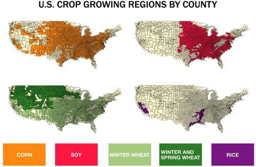
Figure 1. Map of the growing regions for corn, soy, wheat, and rice used in this study. Data used to create the maps are taken from USDA's Quick Stats database.
Download figure:
Standard image High-resolution image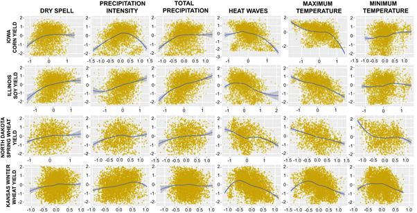
Figure 2. Examples of relationships (or lack thereof) between standardized climate extremes (x-axis), as defined in table 1, and standardized crop yields (y-axis). For each US county in the four states shown, the value for a single year and county is plotted as a single dot, resulting in many data points pooled together. Although all states are used in the main analysis, for illustration purposes, the figure shows the largest producing state for each crop. Kendall's tau was calculated for each crop in each state for each climate variable in the figure. The figures above have statistically significant tau values (p-values <0.05). The top row shows the effects of different extremes on corn yields in Iowa; the second row Illinois soy yields; the third North Dakota spring wheat yields; and the bottom Kansas winter wheat yields. The blue lines are the LOESS best fits surrounded by 95% confidence intervals in darker grey.
Download figure:
Standard image High-resolution imageAs displayed in the LOESS regressions in figure 2, some climate extremes may potentially impact crop yields, and the relationships could possibly exhibit nonlinear behavior. Hence, rather than make any a priori assumptions about relationships between climate and yield (linear, quadratic, etc), we calculate and plot the conditional density functions and high density regions for associated variables of interest (each climate index and yield). This technique takes advantage of the large dataset to establish relationships based on conditional density functions, such that changes in the density (or probability) of a yield value with a climate index can be clearly plotted with no assumptions about the relationship (or existence of a relationship) between yield and climate. For the high density plots, we utilized the R package 'hdrcde' (Hyndman and Yao 2002, Hyndman et al 2013).
3. Results
3.1. Impact of climate variability and extremes on yields across the US
To explore the impact of extremes on yields, the conditional density functions for each crop yield and climate extreme are plotted. Figure 3 shows the relationship between precipitation indices (duration of dry spell, average precipitation intensity, seasonal precipitation, and maximum five-day precipitation) and county average crop yields, pulling together all counties, regardless of irrigated or rainfed, for all five crops (where spring and winter wheat are separated). The plots show both the mode of the yield and the spread of the data conditioned on the climate index.
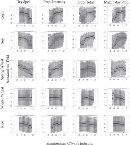
Figure 3. Conditional probabilistic relationships between four different growing season precipitation characteristics (duration of dry spell, precipitation intensity, seasonal total precipitation, and maximum five-day precipitation, respectively in rows) and yields (y-axis) for each crop. Corn is in the left column; soy in the next; followed by spring wheat, winter wheat, and rice. The black dot in each panel of the figure is the mode of the conditional probability of yield for each slice of the climate index values; the darkest grey color contains the 50% highest density region, the medium grey the 95% density, and the light grey the 99% density.
Download figure:
Standard image High-resolution imageRice exhibits little sensitivity to the precipitation indices, with the exception of precipitation intensity; this is likely because rice is predominantly irrigated. Interestingly, this holds true for winter wheat as well, despite being primarily rainfed. Corn and soy demonstrate a decrease in yields with longer duration dry spells during the growing season; this response is less pronounced in wheat. Lower average precipitation intensity, seasonal precipitation, and maximum five-day precipitation all result in declines of corn and soy yields. Spring wheat shows sensitivity to precipitation intensity, displaying a monotonic relationship between mean precipitation intensity and the mode of standardized yields. It is possible that seasonal precipitation and the other precipitation characteristics are positively correlated, resulting in similar relationships with corn and soy yields. For example, seasonal precipitation might be more a function of the precipitation intensity than the number of rain days. Many of the indices that affect yields do so with a threshold behavior rather than a linear or nonlinear relationship. This is seen in maximum five-day precipitation and yields: although yield increases continuously with maximum five-day precipitation, it decreases with the highest recorded value of these climate indices for all crops except rice.
Figure 4 shows the conditional probabilistic relationships between temperature indices and yields for the same crops. As with precipitation indices, rice shows little sensitivity to temperature extremes. Winter wheat shows little variability with the temperature climate indices, with the exception of lower (higher) mean growing season temperatures resulting in higher (lower) yields and a small decline in yields during high maximum temperatures. For spring wheat, heat waves, the number of hot days, and higher maximum temperatures all result in lower yields. For corn and soy, both show an overall decrease in yields with longer duration heat waves, with the decrease occurring abruptly as a threshold. The same is also true for higher maximum temperatures and mean growing season temperatures. Furthermore, corn and soy show increases in standardized yields for the hottest heatwaves and the largest number of hot days, which is counterintuitive and perhaps an artifact of the data.
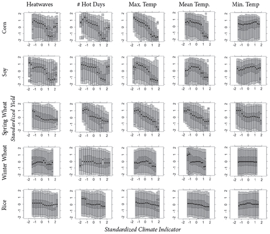
Figure 4. As in figure 3, but for five different temperature characteristics and yields across the growing season for each crop.
Download figure:
Standard image High-resolution imageDifferent relationships exist during the planting season as compared to the growing season (figures S2 and S3 available at stacks.iop.org/ERL/10/054013/mmedia). Corn shows little sensitivity to any of the climate indices. Low planting season precipitation intensities negatively impact soy yields, which is the opposite of the response during the growing season. Spring wheat has similar responses to total precipitation and maximum five-day precipitation, with lower precipitation anomalies resulting in yield decreases. With the exception of the number of hot days in the season, the spring wheat does not exhibit sensitivity to the same temperature indices during the planting season as it does during the growing season. Winter wheat and rice show little sensitivity to any of the climate indices during the planting season, except that rice yield increases with mean temperature and the maximum temperature up to a certain point before it is unaffected by further increases in maximum temperature.
3.2. Impact of irrigation to buffer against climate variability and extremes
Figure 5 repeats the analysis of figure 3, but separates irrigated and rainfed (non-irrigated) agriculture. This analysis is confined to the High Plains states, as they are the ones to report both irrigated and rainfed yields separately. It is clear from this figure that irrigation provides a significant buffer against climate extremes and variability. For example, the decrease in yields with seasonal rainfall for corn and soy is significantly reduced. In fact, for every precipitation index that caused a reduction in yield for a rainfed crop, the effect is either reduced or eliminated for the irrigated crop. This is especially true for the dry spell duration because irrigation water is applied during dry times. In some cases, it significantly extends the threshold before a decline in yield is experienced, as with soy yields and the dry spell duration.
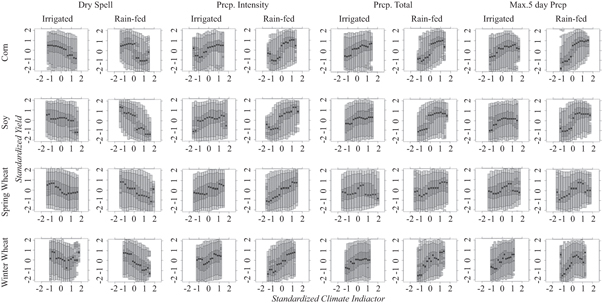
Figure 5. As in figure 3, but irrigated and non-irrigated crop yields are segregated in order to understand the buffering effects of irrigation on yields during climate variability and extremes.
Download figure:
Standard image High-resolution imageFigure 6 extends the analysis of figure 5 for temperature indices. Like precipitation, irrigation reduces the impacts of temperature extremes in many cases. For example, irrigated corn and soy shows a less sensitive relationship with all five temperature indices as compared to rainfed corn and soy. Irrigated corn has a reduction in yield due to the number of hot days in the growing season, but the impact is much more moderate as compared to rainfed corn. This is true for other temperature indices for corn and for spring and winter wheat. The above findings also hold if the climate extremes occur during the planting season (see supplementary material available at stacks.iop.org/ERL/10/054013/mmedia, figures S4 and S5). For each climate index that has an adverse impact on yields, irrigation either eliminates the relationship during the growing season or modulates it through reducing its severity or the threshold at which it occurs. Irrigation can play a large role in buffering against climate extremes during the planting season as well (figures S4 and S5 available at stacks.iop.org/ERL/10/054013/mmedia). Irrigated corn shows no sensitivity to any of the planting season climate indices, with the exception of mean temperature, where there is a very slight decrease in yields with colder planting seasons (figure S5 available at stacks.iop.org/ERL/10/054013/mmedia). Rainfed corn shows decreases in yield in response to many of the climate indices. Irrigated soy and spring wheat also show little response to the climate indices; whereas there is a response in the rainfed crops.
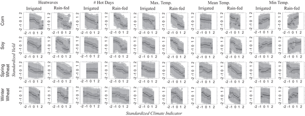
Figure 6. As in figure 4, but irrigated and non-irrigated crop yields are segregated in order to understand the buffering effects of irrigation on yields during climate variability and extremes.
Download figure:
Standard image High-resolution imageIn order to explicitly examine the irrigated yield gains as a function of climate, figures 7 and 8 plot the yield differences (irrigated yield—rainfed yield) against the non-standardized values of the growing season climate indices used in previous figures for precipitation and temperature indices, respectively. Overall, winter wheat shows the least sensitivity in yield differences across the climate indices. As one would expect, the benefit of irrigation increases for corn, soy, and spring wheat with longer dry spells. The yield differences decline with precipitation intensity, total seasonal precipitation, and maximum five-day precipitation, with some increases in the right tail of the climate distributions for spring wheat. These three precipitation indices are correlated with each other in the region where both irrigated and rainfed yields are reported (correlation coefficients ranging from 0.69 to 0.82), making it difficult to attribute which climate variable causes yield responses. Corn and soy show a benefit of irrigation for as maximum temperatures increase until the temperature reaches approximately 34 °C when a decrease in the irrigation benefit is seen. Previous studies have demonstrated a threshold effect of temperature, such as rainfed yields decreasing with temperatures greater than 30 °C (Lobell et al 2013), and it could be that irrigation only moves this threshold rather than eliminates it. A monotonic increase in yield differences exist for spring wheat versus mean growing season temperature. Winter wheat shows a step change in the yield differences when the number of hot days exceeds ten per season.
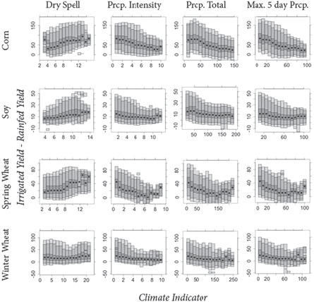
Figure 7. As in figure 3, but the x-axis contains the non-standardized growing season climate index and the y-axis contains the non-standardized difference between irrigated and rainfed yields (bu/ac).
Download figure:
Standard image High-resolution image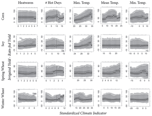
Figure 8. As in figure 7 but for the temperature climate indices.
Download figure:
Standard image High-resolution image
4. Conclusions and discussion
We are able to estimate the impact of climate extremes on crop yields, graphically, by pooling all the counties together, which significantly increases the number of data points in the tails of the distributions and enhances statistical power. This study provides a good generalization of US-wide impacts of climate extremes on crop production. Our method of analysis pools together crops grown across a range of climates given the large size of the United States. This assumes that farmers plant crop varieties particularly suited to their local climate, so that standardized anomalies have similar impacts on yields regardless of the mean climate. This may not reflect certain thresholds of extremes that exist regardless of cultivar choice. For example, corn and soy yields have been shown to have an optimum growing temperature of 29 °C and 30 °C, respectively; temperatures above this threshold result in yield decreases (Schlenker and Roberts 2009).
Irrigation is shown to have a beneficial impact in increasing yields and provides a significant buffer against both precipitation and temperature-derived climate indices. For example, the mode of yield differences is over 100 bu/ac for growing season maximum temperatures of 33 °C. The physical mechanism for why irrigation changes the crop response for temperature-related indices is an open question. This could be because temperature affects the potential evapotranspiration and irrigation would reduce water stress induced by high potential evapotranspiration. However, it also could be that there is a local decrease in temperature due to evaporative cooling: Bonfils and Lobell (2007) demonstrated a decrease in maximum temperature in irrigated regions. Because this work uses county-average temperature data, there could be local cooling that is averaged out at the county scale. Identifying the exact mechanism would require detailed process-based modeling at the field scale. In addition, canopy temperatures experienced by the crop may differ from the measured air temperature at 2 m. Siebert et al (2014) showed that irrigated crops can have a canopy temperature 2 °C cooler than the measured and rainfed crops can have a canopy temperature up to 5 °C higher. These differences between the temperature experienced by the crop and that measured introduces uncertainty into the analysis used here, but also provides some insight into why irrigated crops may behave differently than rainfed under temperature extremes.
Each climate index was analyzed independently to evaluate the impact of that extreme on crop yields. It is possible that some of these climate indices are correlated, and it is therefore difficult to know which (or if both) variables are determining the change in crop yields. For example, precipitation intensity, seasonal total precipitation, and maximum five-day precipitation are all correlated with one another, with correlation coefficients ranging from 0.69 to 0.82. The methodology in this paper focuses on correlative relationships and the results do not necessarily imply causation. In addition, some of the climate indices are possibly correlated among each other: e.g., the probability of a heat wave during a dry period may be higher than climatology. This leads to interesting questions of which extreme primarily affects the crop yield or if the combination of multiple extreme indices results in further yields decreases. Further work could entangle this by evaluating the combined effects of concurrent extremes, such as drought and heat waves, as well as solo temperature and precipitation events to ascertain how the yield response differs. When translating these results to agricultural vulnerability to climate, concurrent extreme values should be considered in order to not overestimate the yield declines due to climate extremes. Other variables besides climate will influence crop yields, such as soil texture, soil depth, cultivar, and farming practices, all of which are not considered in this study. It is possible that these variables could be causing the large spread in crop responses to climate, and it remains an open question how large a role these other variables play.
The strengths of the methodology used to quantify the distribution of crop yield responses to climate indices are also its limitations. The graphical technique allows for a complete representation of all the data, which can allow for a better understanding of the stochastic nature of crop responses to climate. However, it does not provide any insights into the physical mechanisms of the crop response nor does it demonstrate causation, only correlation. Much of the interpretation is visual rather than quantitative. The methodology allows for relatively quick computational displays of relationships between two variables in large datasets, which can then allow researchers to focus on the variables of interest in a more quantitative framework.
These analyses were all performed for the United States, which covers a number of climate zones. As such, these results are believed to be robust predictors of the impact of climate on the yields of wheat, soy, rice, and corn in the US. However, before extrapolating the relationships globally, they should be confirmed in other geographic regions where relatively fine spatial scale agricultural yield data is available. The spatial resolution needed makes this difficult: country-level agricultural production and yields are readily available, but it would be difficult to ascertain what was irrigated and what was rainfed. It would also be difficult to tease out the impact of climate extremes on yields given that the extremes rarely occur over the entire growing region, so that some cropped areas would be affected and others would not. Unfortunately, sub-national data outside the US is often difficult to obtain except at field research sites. This is challenging as there may be only one or two of each climate extreme in the historical record at each site, which makes establishing any impact on yields statistically problematic.
It is likely that extremes will increase in intensity and frequency in the coming decades. How these extremes will impact crop production is of considerable interest as it is also expected that population will continue to grow, potentially stressing an already stressed food supply. Based on these results, irrigation can provide a potent buffer against both precipitation- and temperature-related climate extremes. However, any expansion of irrigation must be considered against the available water resources, both in terms of the mean and the extremes, so that a reliable food supply is not prioritized at the expense of reliable water resources. In the US, many parts of the country experience water scarcity due to both climate variability (droughts) and anthropogenic water use. In addition, agricultural runoff can decrease water quality downstream. Irrigation should therefore be considered as one way of buffering against climate extremes where appropriate; other measures such as increased grain storage capacity should also be considered given the expected increased exposure of the food system to extreme events.
Acknowledgments
The authors gratefully acknowledge Upmanu Lall for recommending the moving window approach for the yield standardization.