
Abstract
Sizing storage for rainwater harvesting (RWH) systems is often a difficult design consideration, as the system must be designed specifically for the local rainfall pattern. We introduce a generally applicable method for estimating the required storage by using regional regression equations to account for climatic differences in the behavior of RWH systems across the entire continental United States. A series of simulations for 231 locations with continuous daily precipitation records enable the development of storage–reliability–yield (SRY) relations at four useful reliabilities, 0.8, 0.9, 0.95, and 0.98. Multivariate, log-linear regression results in storage equations that include demand, collection area and local precipitation statistics. The continental regression equations demonstrated excellent goodness-of-fit (R2 0.96–0.99) using only two precipitation parameters, and fits improved when three geographic regions with more homogeneous rainfall characteristics were considered. The SRY models can be used to obtain a preliminary estimate of how large to build a storage tank almost anywhere in the United States based on desired yield and reliability, collection area, and local rainfall statistics. Our methodology could be extended to other regions of world, and the equations presented herein could be used to investigate how RWH systems would respond to changes in climatic variability. The resulting model may also prove useful in regional planning studies to evaluate the net benefits which result from the broad use of RWH to meet water supply requirements. We outline numerous other possible extensions to our work, which when taken together, illustrate the value of our initial generalized SRY model for RWH systems.
Export citation and abstract BibTeX RIS

Content from this work may be used under the terms of the Creative Commons Attribution 3.0 licence. Any further distribution of this work must maintain attribution to the author(s) and the title of the work, journal citation and DOI.
1. Introduction
In recent years, rainwater harvesting (RWH) has attracted increased attention for various reasons including its use as an alternative water supply and for urban water management, notably control of stormwater. RWH has maintained its importance as a water source for small scale agricultural needs and as a primary water source in remote locations in rural areas and on islands. In the past few decades, RWH has also become a popular supplemental (and generally non-potable) water source in urban and suburban areas in a wide range of climatic and socio-economic environments. The history of RWH, and evolution of system types, forms, and objectives has been well covered in the literature (see reviews by Boers and Ben-Asher 1982, Pandey et al 2003, Basinger et al 2010).
The elements of design of RWH systems vary according to the designer's goals for system performance. A designer interested in supplying potable water will value reliability, a suburban gardener may value the water saving efficiency, and a stormwater engineer may value capture efficiency. These disparate objectives and interests have led to the use of different metrics and constraints upon which to assess RWH system performance, though the physical components of the system-collection area, conveyance, and storage—remain largely consistent. In most cases, the most important and difficult design decision is how much storage capacity to build. Being unable to change the rainfall pattern in the location of the planned RWH system, designers focus on the system components and parameters they can control, namely, the collection area, storage volume, and demand level. But rainfall patterns have a strong relationship to the overall functioning of the system, and a better understanding of the effect of the rainfall pattern on system performance could inform system design, notably in sizing storage. While there is no substitute for a detailed engineering design study at a given project location, there would be great utility in a simpler and more generally applicable method of preliminary RWH storage capacity estimation.
1.1. RWH cistern sizing and simulation
RWH sizing approaches vary considerably in approach, methodology, the type of rainfall data used and the way in which those rainfall data are used. The simplest sizing methodologies are based on a simple water balance or a mass curve analysis (Handia et al 2002). Early versions of these analyses were performed with monthly rainfall records or average monthly rainfall (Watt 1978, Keller 1982). Algorithms for simulating the behavior of RWH systems using monthly rainfall records quickly replaced these methods (Schiller and Latham 1987). More recently, continuous simulation methods using daily rainfall records have been used to explore RWH system behavior (Fewkes 2000, Palla et al 2011), optimize performance relative to system cost (Liaw and Tsai 2004), or analyze potential potable water savings (Ghisi and Ferreira 2007). More detailed models investigating system performance under a complex demand pattern (i.e. multiple end uses being used at different times) have used hourly (Villarreal and Dixon 2005) or even 5 or 6 min rainfall data (Coombes and Barry 2007, Herrmann and Schmida 2000). Other RWH sizing and simulation approaches use semi-parametric (Cowden et al 2008) or nonparametric (Basinger et al 2010) stochastic precipitation generators to generate synthetic rainfall series to entirely replace or fill gaps in rainfall records. Guo and Baetz (2007) used an analytical approach from stormwater detention theory using the statistical characteristics of a continuous rainfall record (event totals, storm durations, and inter-event storm arrival times) as inputs to generate a complex series of equations enabling computation of necessary storage.
Ultimately, all of these approaches rely on local precipitation records, either as a hydrologic input or for computing parameters needed as an input to a stochastic precipitation model. The studies cited above have investigated how design parameters (storage volume, collection area, demand, etc) affect various measures of system performance (reliability, water saving efficiency, overflow volume), but relatively little effort has been devoted to determining how characteristics of a rainfall record, other than mean rainfall, affect overall RWH system performance. Furthermore, previous modeling efforts have focused on individual systems in a particular location, but little effort has been given to the generalization of approaches for sizing RWH systems across broad geographic regions that experience significant variations in climatology.
1.2. Using hydrologic statistics to study system behavior
The first step in being able to determine how characteristics of the rainfall pattern affect system performance is to describe the RWH system performance mathematically. Repeated simulations can generate empirical relationships between the design parameters and performance metrics to define local performance curves (Fewkes 1999). Regression approaches have been used to generate equations relating some system parameters. Liaw and Tsai (2004) used regressions to define isoreliability economic tradeoff curves between collection area and storage volume costs.
Lee et al (2000) developed a regression equation to relate the major system parameters (irrigation demand, collection area, storage) and performance (reliability) for a single agricultural RWH site in China. Since only a single site is considered, the character of the hydrologic input (rainfall) is effectively built into the regression model. Commenting on this study, Guo and Baetz (2007) remark, 'One series of such simulation modeling and regression analysis would have to be conducted for each geographical location of interest. The resulting regression equations would be applicable for only the locations studied.' Ironically, Guo and Baetz (2007) demonstrated analytically that differences in RWH system performance between locations can be explained by differences in the statistical parameters of the rainfall sequence.
Our primary hypothesis is that a multivariate regression framework similar to Lee et al's might lead to RWH relationships with greater geographic generality by also including certain rainfall statistics in the regression. Multivariate regression has been used to generalize the behavior of reservoirs based on the statistical parameters of their inflow sequence. For example, McMahon et al (2007) use regional regression to estimate theoretical reservoir storage requirements for a particular streamflow station by using reservoir yield, reliability and various annual streamflow statistics as predictive variables (on a global geographic scale). Regional regression approaches have also proven useful in estimating other hydrologic parameters over broad geographic areas, most notably, streamflow (Vogel et al 1999).
The RWH system is conceptually similar to a surface water reservoir system fed by a stream, though there are important differences. Both have a fixed storage capacity, a characteristic volumetric demand, and a volumetric inflow determined by natural hydrologic processes. A surface water reservoir's inflow is determined by the volumetric flow of its influent streams that collect rainfall over the contributing watershed, which is analogous but more complex than precipitation falling on a RWH system's collection area.
The storage–reliability–yield (SRY) framework from reservoir analysis (Vogel and Stedinger 1987, Vogel and McMahon 1996, McMahon and Adeloye 2005) may be useful for RWH studies because it can handle a range water supply yield and reliability cases. The relationships of the storage capacity, reliability and demand (yield) variables have been explored for RWH systems (Schiller and Latham 1987, Fewkes 2000, Villarreal and Dixon 2005), though not specifically in a SRY context. Given a daily rainfall record, a series of behavioural simulations can determine an empirical SRY relationship, which would provide a starting point for regression analysis.
Though some similar methodology is used, this study is significantly different from past regional hydrologic regression studies for a variety of reasons. Importantly, to our knowledge this is the first study which seeks to develop generalized SRY relationships for RWH systems that could be applied across an entire continent. Our approach, while analogous to the approach used by others for developing generalized SRY relationships for surface water supplies fed by rivers, differs in nearly every aspect. Unlike the early studies by Vogel and Stedinger (1987) and Vogel and McMahon (1996) and many subsequent studies summarized by McMahon and Adeloye (2005), which developed generalized SRY relationships based on hypothetical, theoretical inflow series, our approach employs actual rainfall series for 231 locations as inflows to the RWH systems. Similarly, many previous SRY relationships for surface water reservoirs incorporate critical assumptions regarding the probabilistic structure of both reservoir inflows and resulting storage capacities. Our study of RWH systems does not make any such probabilistic assumptions. Additionally, while the watershed area draining to a reservoir or stream gage location is essentially fixed, the collection area for a RWH system is an important design parameter, and any regression models developed should be normalized to collection area such that collection area can be easily changed.
Our primary goal is to establish a generally applicable, technically rigorous, and easily applied method for estimating the required storage for a planned RWH system with user-specified collection area, and a desired demand and reliability. Our approach is to use multivariate regression to generate regional equations relating storage capacity to demand level at given reliabilities, as well as certain parameters of the observed daily rainfall sequences to account for climatic differences across the entire geographic region of the continental United States.
2. Methods
We simulate RWH systems that collect rainfall from a rooftop collection area with storage in a closed cistern and constant daily demand (yield), which may reasonably approximate a system designed to meet daily toilet flushing and/or other constant (likely indoor) daily needs. Long records of daily precipitation data for the 231 locations shown in figure 1 across the continental United States were used to simulate RWH systems and to generate SRY relationships. Simulations generated sets of points defining a fixed reliability storage–yield (SY) curve for several useful design reliabilities (80%, 90%, 95%, and 98%). Then, the SY data were used in a regional regression approach to obtain generalized equations for estimating storage for RWH systems using system parameters and daily rainfall statistics.

Figure 1. Map of regional divisions and locations of 231 first-order precipitation gages used in this study.
Download figure:
Standard image High-resolution image2.1. Simulation of RWH systems
A set of 231 first-order precipitation gages shown in figure 1 from the National Weather Service's Cooperative Station Network with high-quality daily records were selected as hydrologic inputs for simulation. The stations are well distributed across the continental United States and have a median record length of 59 years. The Yield-After-Spillage algorithm, widely used in the RWH literature (Jenkins et al 1978, Schiller and Latham 1987, Fewkes 1999, Mitchell 2007, Palla et al 2011), is selected for the simulations. We assume the runoff coefficient of the collection area to be one, and no first flush is modeled. The precipitation gages report snow as liquid equivalent, so simulations are continuous even in sub-freezing conditions impractical for actual RWH operation.
Each simulation, run for a single combination of yield and storage, tracks daily storage and whether the daily yield is met each day. The number of days with failure is recorded, and used to compute reliability, qt given by

where qt is reliability, df is the number of days with failure to meet full demand in the simulation, and n is the number of days simulated. All simulations are run for a unit rainfall collection area Ac of 1 m2. Additionally, the yield is normalized by the mean daily rainfall of each station to generate the nondimensional yield ratio α, which describes the average fraction of available water used and is given by

where D is the constant volumetric daily demand (L d−1), μ is mean daily precipitation (mm d−1), and Ac is collection area (m2).
An algorithm iterated through values of storage until the desired reliability, qt (e.g. 0.9), was reached for the given yield ratio α. A set of 20 simulations with α ranging from 0.05 to 0.99 defines a constant reliability curve. The reported storage volume is normalized to collection area to generate the physical storage ratio, Sr (3). Though Sr may have any unit of length (e.g. meter), Sr is expressed here in units of centimeters, but is more meaningfully understood as m3 of storage per 100 m2 of collection area.

where Sr is the physical storage ratio, K is total storage capacity (m3). Storage is expressed in this manner instead of the dimensionless storage ratio common to reservoir literature (McMahon and Adeloye 2005), which in this case would require further dividing by the mean annual rainfall, μ. This choice was made because collection area is an important system parameter, and further embedding μ into the definition of the storage variable would make calculating storage capacity more cumbersome. Furthermore, this form allows regressions to be fit to a variable (Sr ) free of rainfall parameters, meaning rainfall parameters will only be on the right hand side of the regression, thus avoiding potential spurious correlation due to rainfall variables common to both sides of the equation.
The constant reliability curves can effectively describe the full SRY relationship when plotted. Figure 2 shows a set of simulated reliability contours generated using precipitation data from Los Angeles, CA. Figure 3 displays the 0.9 reliability contour from several locations to illustrate the wide variation in the shape and position of the SY curve between stations.
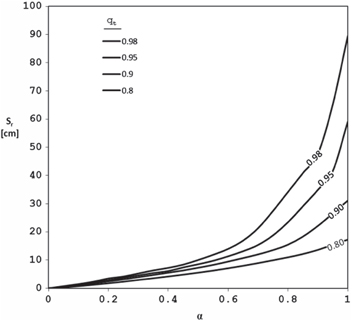
Figure 2. Storage–yield relationship for four reliability contours for a single station (Los Angeles, CA).
Download figure:
Standard image High-resolution image
Figure 3. Variability of the Sr –α relationship across stations for the qt = 0.9 reliability curve.
Download figure:
Standard image High-resolution image2.2. Regression modeling approach
We use multivariate ordinary least squares (OLS) regression as the method of generalizing the SY relationships across the entire US. The two goals of the regression modeling are (1) to determine which precipitation summary statistics most strongly influence differences in the SRY relationship between sites, and (2) to develop a generalized predictive model for estimating required system storage.
The regression equation is of the general form

where Sr denotes the physical storage ratio, Xi , i = 1...m, describe physical system parameters such as the yield ratio α, defined in (2) and Yj , j = 1...n, describe local climate statistics.
The model in (4) is log-linear because taking the natural logarithm of (4) results in
The simulation of the RWH systems kept fixed all of the major system parameters except storage and demand on the system. Since storage is the dependent variable of the regression, the only system parameter (Xi ) that needs to be included in the regression is a representation of demand. Several expressions of average demand or yield of the system were investigated, but the yield ratio, α, from (2) was selected as simplest and most general, and has the benefit of having a constant domain across stations.
One difficulty with using yield ratio, α, is that the isoreliability SY curves on which the regressions are based are highly nonlinear, especially as reliability approaches 1. We sought to investigate if the Sr –α relationship could be linearized to enable application of OLS regression methods. Even when both variables were logarithmically (base e) transformed, nonlinearity persisted. A single site regression analysis was performed for all stations to obtain the form of the regression model describing the relationship between Sr and α for a constant reliability curve. The model in (6) resulted in a fit with R2-adjusted above 0.99 for all stations and reliabilities

While the model in (6) is no longer log-linear, the transformation caused by the d parameter can still be incorporated into a log-linear model. Replacing ln(X1) in (5) with [−ln(α)]d , and exponentiation of both sides leads to

Equation (7) relates Sr , α, and some precipitation parameters that will be determined via regression analysis. The precipitation statistics investigated in the regressions include standard statistics calculated from the full record of daily precipitation depths, and also from the wet-day series (left censored to remove zero and trace values). Also included is the lag-1 serial correlation (autocorrelation) coefficient, ρ, along with a transformation (1 + ρ)/(1 − ρ) familiar to reservoir analysis (see Phatarfod 1986, and Vogel and McMahon 1996 for two independent derivations of this transformation).
These parameters were added to the regressions using a staged regression analysis to determine how the addition of each parameter improved the overall goodness-of-fit. Regression models were developed for each reliability case using all stations in the study region. Then, the stations were broken down into three regions (divided along major river basin boundaries) shown in figure 1 to see how regressions might improve. Table 1 displays the average precipitation characteristics of the regions, and all stations.
Table 1. Average precipitation characteristics of the three regions, and all US stations.
| Region | Stations (n) | μy Mean (mm yr−1) | 10th percent. (mm yr−1) | 90th percent. (mm yr−1) | Cv | ρ | P(x = 0) | μw (mm d−1) | σw (mm) | Cvw |
|---|---|---|---|---|---|---|---|---|---|---|
| East | 97 | 1094 | 835 | 1382 | 0.229 | 0.114 | 0.648 | 8.71 | 12.2 | 1.50 |
| Midwest | 82 | 757 | 381 | 1327 | 0.280 | 0.145 | 0.740 | 7.91 | 11.9 | 1.36 |
| West | 52 | 417 | 159 | 984 | 0.268 | 0.225 | 0.780 | 4.94 | 6.7 | 1.42 |
| All US | 231 | 820 | 292 | 1329 | 0.256 | 0.150 | 0.710 | 7.58 | 10.8 | 1.40 |
Notes: μy denotes the mean annual rainfall of the stations, shown with the 10th and 90th percentiles of the stations in each region. Cv denotes the coefficient of variation, ρ denotes lag-1 correlation of daily rainfall depth, and P(x = 0) denotes the daily probability of zero rainfall. μw , σw , and Cvw denote the mean, standard deviation and coefficient of variation, respectively, of the daily wet-day rainfall series.
3. Results
An effort was made to make the resulting models as simple as possible, by adding relatively few precipitation parameters. An initial search was performed on the precipitation variables to determine which had the most explanatory power in a single parameter regression. Using the data from all stations for the 90% reliability case, the transformation in (6) was applied, with d = 0.667 resulting in the highest goodness-of-fit. In each case shown in table 2, the following model containing the transformed α and a single precipitation parameter, Y, was fit to the data:

Table 2. Goodness-of-Fit of regressions (adjusted R2), and T-ratio for a single precipitation parameter model (8) with regression coefficients for the 90% reliability case.
| Coefficients | ||||||
|---|---|---|---|---|---|---|
| Parameter, Y | Description | R2 adj. | T-ratio for Y | a | b | c |
| σw | Standard deviation, wet-day | 91.3 | 57.42 | 0.4056 | −2.307 | 0.7867 |
| μw | Mean, wet-day | 91.1 | 55.47 | 0.6987 | −2.307 | 0.7801 |
| x0.5, w | Median, wet-day | 89.8 | 46.15 | 1.434 | −2.307 | 0.6706 |
| σ | Standard deviation | 89.0 | 40.46 | 2.581 | −2.306 | 0.5395 |
| (1 + ρ)/(1 − ρ) | Transformation of ρ | 87.7 | 31.33 | 1.693 | −2.306 | 1.713 |
| ρ | Serial correlation coeff., lag-1 | 87.2 | 27.14 | 3.312 | −2.306 | 0.5599 |
| μ | Mean | 87.0 | 25.56 | 2.021 | −2.305 | 0.2936 |
| Cv | Coefficient of variation | 85.5 | 10.76 | 1.763 | −2.305 | 0.3898 |
| P(x = 0) | Dry day probability | 85.5 | 10.56 | 2.447 | −2.305 | 0.6727 |
| γ | Skewness | 85.3 | 6.65 | 1.818 | −2.305 | 0.2171 |
| Cvw | Coeff. of variation, wet-day | 85.3 | 7.07 | 1.986 | −2.305 | 0.6356 |
| κ | Kurtosis | 85.2 | 5.6 | 1.869 | −2.305 | 0.0840 |
| γw | Skewness, wet-day | 85.2 | −3.92 | 2.415 | −2.305 | −0.1653 |
| κw | Kurtosis, wet-day | 85.1 | −3.15 | 2.367 | −2.305 | −0.0521 |
The resulting regression coefficients and adjusted R2 values are also reported in table 2, along with the T-ratio for the precipitation parameter Y. The parameters described with a subscript 'w' indicate the parameter is calculated from the wet-day record. All others are calculated from the full record daily rainfall series (depth expressed in mm).
Table 2 orders precipitation parameters from highest adjusted R2 to lowest, indicating that of the precipitation statistics considered, σw and μw have the most explanatory power. We note that μ is embedded in the definition of α (see equation (2)), so using it in regression models might introduce concerns over multicollinearity. However, the recent experiments performed by Kroll and Song (2013) document that in situations when the model form is unknown, as is the case here, it is reasonable to employ the multivariate OLS regression methods used here, even in the presence of multicollinearity, and especially considering the large samples used to develop these models. In any case, several parameters outperform μ.
Table 3 illustrates the best regressions with two precipitation statistics included, for all four reliability cases, when all stations are included. All of the regressions in table 3 take the form of (9), with σw and (1 + ρ)/(1 − ρ) as the two precipitation parameters

Table 3. Regression coefficients for equation (9) for the four reliabilities, and measures of regression performance including: variance inflation factor (VIF), standard error (SE), adjusted R2 (R2 adj.), as well as T-ratios for the parameters.
| Regression coefficients | ||||||||
|---|---|---|---|---|---|---|---|---|
| Reliability | a | b | c1 | c2 | d | Max VIF | SE | R2 adj. |
| 0.80 coeff. | −0.778 | −2.309 | 0.971 | 2.514 | 0.667 | 1.064 | 0.247 | 0.966 |
| T | −31.1 | −340.5 | 109.7 | 85.1 | — | — | — | — |
| 0.90 coeff. | 0 | −2.566 | 0.958 | 2.599 | 0.642 | 1.064 | 0.254 | 0.977 |
| T | — | −360.5 | 238.1 | 102.2 | — | — | — | — |
| 0.95 coeff. | 0.762 | −2.934 | 0.952 | 2.433 | 0.577 | 1.064 | 0.247 | 0.971 |
| T | 30.1 | −371.2 | 105.6 | 80.7 | — | — | — | — |
| 0.98 coeff. | 1.768 | −3.552 | 0.938 | 2.177 | 0.483 | 1.063 | 0.266 | 0.969 |
| T | 64.1 | −361.1 | 97.3 | 66.8 | — | — | — | — |
Regression models using three precipitation parameters were investigated, but the small improvement in goodness-of-fit did not justify the added complexity. Additionally, the model coefficient for the third precipitation variable was often less significant than the regression constant, a, as measured by its T-ratio. Figure 4 compares the predicted versus simulated values of Sr for the four models summarized in table 3.

Figure 4. Predicted RWH Storage capacity (Sr,pred) versus simulated (Sr,sim) values for the four reliability models summarized by equation (9) and table 3 based on all 231 precipitation stations.
Download figure:
Standard image High-resolution imageTable 4 summarizes the regression coefficients and fits for the three regions for each reliability case. The East, Midwest, and West regions use regression equations (9)–(11), respectively


Table 4. Regressions and fits for the three regional regression models, each for four reliabilities.
| Regression coefficients | |||||||||
|---|---|---|---|---|---|---|---|---|---|
| Region | Reliability | a | b1 | c1 | c2 | d | Max VIF | SE | R2 adj. |
| East | 0.80 | −1.106 | −2.168 | 1.054 | 2.253 | 0.675 | 1.286 | 0.129 | 0.989 |
| East | 0.90 | −0.289 | −2.694 | 1.062 | 2.818 | 0.589 | 1.288 | 0.151 | 0.988 |
| East | 0.95 | 0.567 | −3.221 | 1.047 | 2.934 | 0.516 | 1.290 | 0.165 | 0.987 |
| East | 0.98 | 1.640 | −3.735 | 0.932 | 3.176 | 0.468 | 1.248 | 0.222 | 0.979 |
| Midwest | 0.80 | −0.539 | −2.499 | 0.771 | 0.967 | 0.655 | 1.016 | 0.183 | 0.982 |
| Midwest | 0.90 | 0.330 | −2.618 | 0.714 | 0.931 | 0.669 | 1.006 | 0.189 | 0.983 |
| Midwest | 0.95 | 0.885 | −2.831 | 0.744 | 0.896 | 0.630 | 1.010 | 0.179 | 0.985 |
| Midwest | 0.98 | 1.749 | −3.332 | 0.779 | 0.779 | 0.537 | 1.016 | 0.202 | 0.982 |
| West | 0.80 | −0.831 | −2.208 | 1.570 | 1.185 | 0.696 | 2.583 | 0.272 | 0.965 |
| West | 0.90 | −0.124 | −2.288 | 1.431 | 1.481 | 0.695 | 2.608 | 0.240 | 0.974 |
| West | 0.95 | 0.812 | −2.631 | 1.054 | 2.068 | 0.613 | 1.463 | 0.243 | 0.973 |
| West | 0.98 | 1.814 | −3.211 | 1.033 | 1.783 | 0.505 | 1.489 | 0.248 | 0.974 |
Note: Use (9) for East, (10) for Midwest, and (11) for West.
In general, the three regional regression models summarized in equations (9)–(11) and table 4 perform somewhat better than the regressions based on all 231 stations, especially the East and Midwest.
4. Discussion
4.1. Significance of parameter selection
The high R2 values (0.96–0.99) associated with these regression equations show that including a few relatively simple daily rainfall statistics can generate surprisingly accurate equations for estimating required storage for RWH systems across broad geographic and climatic regions. Even though the precipitation data set includes a wide range of climate types, the regression equations explain much of the difference in the Sr –α relationships between sites with only a few rainfall statistics added to the model.
The most useful rainfall parameter appears to be the standard deviation of the wet-day series of daily rainfall depth. The coefficients for σw are positive in all of the regression equations presented, so required storage increases as σw increases. These results are in accordance with an intuitive understanding of how RWH systems respond to rainfall parameters. Given an average rainfall depth for a site, the minimum storage volume for a RWH system would be achieved if local rainfall delivered exactly the average rainfall depth on every day. As rain does not fall every day, the minimum storage would be achieved if the rainy days were evenly spaced, and all rainy days had equal rainfall depth. Increasing variability in either the wet-day precipitation depth (i.e. σw or perhaps more precisely Cvw ), or the relative length of dry and wet spells (i.e. increasing autocorrelation) increases the storage volume. Vogel and McMahon (1996) show that (1 + ρ)/(1 − ρ) is effectively a factor which accounts for the inflation in the variance of a sample mean due to serial correlation of a series. Thus, this factor is closely related to the variance of the wet-day series, which may indicate why it was a helpful addition to the regional regressions.
When considering three sub-regions of the United States, the regression fits improved, presumably due to greater homogeneity in overall hydroclimatic characteristics, especially mean precipitation depth (see table 1), but parameter selection did vary between regions. The most powerful precipitation parameters in a regression will be those that best explain differences in the behavior of RWH systems between locations. For example, the West regression models showed a preference for μw over σw , which indicates that the wet-day mean rainfall was being used to explain differences in system behavior. This finding may be indicative of the wide climatic variation in the sample of West stations.
4.2. Use of regression equations and caveats
Some significant caveats should be considered when using these equations to estimate storage size of RWH system. Notably, the simulation methodology assumed constant daily demand, perfect collection efficiency, and no first flush device. Furthermore, the expression of time-based reliability indicated only the percentage of failure days within the entire record, but not the distribution of those failure days within the simulation period, or a particular period or season of interest. On the other hand, the time-based reliability is more conservative than volume-based reliability given constant daily demand. Extra caution should be exercised in using the results of the regression as α approaches 1 due to the extreme curvature of the SY curves.
Although the resulting equations were developed over very broad climatic and geographic regions of the United States, we do not recommend use of these equations outside the range of climatic characteristics summarized in table 1, or areas with climates considered extreme for the region (e.g. microclimates). It is always dangerous to extrapolate statistical models outside the range of variables used for their calibration. In that case, simulation methods to generate a set of local performance curves would be preferred. The regression equations presented may be potentially applicable in other geographic regions with similar latitudes or climates if climate characteristics are similar to those in table 1. Developing new regressions for other areas would be preferable, of course. Site selection for any future regional regressions should likewise take care not to include sites with microclimates or climates aberrant from the general character of the region.
In most cases, many of these limitations and caveats raised here may be remedied or at least addressed by choosing an appropriate factor of safety in selecting the storage volume.
5. Validation and sample calculation
In order to validate the regression models, an example compares predicted SY curves to simulated SY curves for a station not included in the development of the model. The station selected is Spartanburg 3 SSE in Spartanburg, South Carolina, which has a 30 yr daily precipitation record, and mean rainfall of 3.37 mm d−1 (1232 mm yr−1). The simulated RWH system has a collection area of 100 m2. Based equation (2), with Ac = 100 m2 and μ = 3.37 mm, the maximum supportable demand (α = 1) is 337.3 l d−1. Additionally, ρ = 0.123, and σw = 15.5 mm. Figure 5 presents the simulated SY curves for the four reliabilities for this particular station as dashed lines for comparison with the results based on two different regressions. Using the values of μ, σw , ρ, Ac , the values of storage capacity, K, were computed from the full US and East (Spartanburg's region) regression models for a wide range of α values for each reliability case.

Figure 5. Simulated and regression model predicted SY curves for Spartanburg, SC, four reliabilities.
Download figure:
Standard image High-resolution image
In general, there is strong agreement between the simulated and predicted SY curves, and the East regression model outperforms the US model in most cases. In this particular validation, the predicted values are often slightly higher than the simulated values, but if another station were used in a validation, this may not be the case.
Now, consider a specific design case. Suppose the proposed system is used to meet toilet flushing needs with constant daily demand, D = 150 l d−1. Using equation (2) with mean daily rainfall of 3.37 mm d−1, the yield ratio is

With this value of α from (13) and the rainfall parameters ρ and σw , equation (9) can be used to calculate Sr using the coefficients in table 3 (US model) or 4 (East region model) for any of the four reliability cases. The regression equation output is expressed as Sr , which must be converted to storage capacity, K (m3) using equation (3), though in this case with Ac = 100, K = Sr . Alternatively, K can be calculated directly by substituting (3) into (9), resulting in:

Suppose the designer desires a reliability between 90% and 95%. Using the given rainfall statistics, collection area, demand, and appropriate regression coefficients from tables 3 and 4, values K are shown in table 5 for both the simulation and the two regression models.
Table 5. Simulated and calculated storage K (m3) for sample location with Ac = 100 m2, 90 and 95% reliability cases for demand of 150 l d−1.
| Reliability qt | K simulation | K East model | K US model |
|---|---|---|---|
| 0.90 | 2.43 | 2.55 | 2.78 |
| 0.95 | 3.46 | 3.56 | 3.94 |
Given the results in table 5, the designer can roughly estimate required storage as between 2.6 and 4 m3. For final system sizing, a more detailed engineering study is of course recommended.
6. Summary: conclusions, recommendations and extensions
6.1. Conclusions
Determination of the required storage for a RWH system often presents a difficult design challenge. This study considered the problem of how to simplify the calculation of storage capacity by incorporating the information about RWH systems provided by a very wide range of simulation experiments across a very broad range of climatic conditions. Considering a RWH system as a storage reservoir, a daily RWH simulation model was used to develop generalized empirical SRY relationships at the 231 US locations shown in figure 1. To our knowledge, this is the first example of such a generalized RWH SRY relationship based on a continental dataset of precipitation measurements.
We hypothesized that differences in SRY relationships for RWH systems between stations could be explained by daily rainfall statistics, which make possible a generalized regression model capable of calculating required storage anywhere in the study area (continental United States). We show that by including daily rainfall statistics along with RWH system parameters into a multivariate log-linear regression framework can lead to a surprisingly powerful generalized SY equation at several useful reliabilities. Additionally, the regression analysis can highlight which characteristics of the rainfall distribution (other than the mean) most strongly affect RWH performance. Notably, standard statistics of the wet-day rainfall series had considerable explanatory power in the regressions, including its mean and standard deviation, μw and σw , respectively.
The regression models presented can be used to obtain a preliminary estimate of how large to build a storage tank based on desired yield and reliability, collection area, and local rainfall statistics. Since the climatic variables selected are relatively easily calculated with even incomplete daily precipitation records, the equations may be useful to wide range of users in estimating required storage. The rainfall statistics may be obtained from maps in regions with sparse or no rainfall data. Pooling of rainfall data from maps and localized short records to obtain blended estimators of rainfall statistics for use with our models may also prove useful. Mapped rainfall parameters would also allow using the equations to map storage requirements across a region.
Our framework could be extended to incorporate more RWH system design parameters, or test a broader set of precipitation statistics. One way would be to run many simulations with different values for runoff coefficients, first flush volume, and include those parameters in regression models. Incorporation of a broader set of daily rainfall statistics into the analysis could lead to improved regressions, but ease of calculation is an important consideration. Notably, measures of the variance of rainfall and measures of timing and/or seasonality may slightly improve regression fits, but substantial improvements are unlikely. Some initial tests indicate that the scale parameter of the Pearson-III distribution fitted to the full record series may slightly outperform σw (with which it is highly correlated).
6.2. Recommendations and extensions
There are a number of useful extensions to the generalized SRY relationships for RWH systems introduced here which we describe below. When taken together, the following extensions outline a research program with numerous benefits which would be difficult without the model developed here.
Within the context of water resource systems design and management, the derived RWH relationship could be used to optimize the operation, management and design of RWH systems. The regression equations could be used in planning studies which seek to examine cost-supply tradeoffs in urban settings, or evaluate the benefits of additional household water supply in rural areas or areas underserved by water infrastructure.
The expressions introduced here are useful for evaluating the impact of climate change on the performance (the reliability and/or yield) of existing or proposed RWH systems given expected changes to daily rainfall pattern. To the extent that downscaled climate models can predict changes in the daily precipitation distribution, regional regressions of this form could help predict changes in storage and/or RWH system yield under changing climate conditions. In that case, simpler models using only parameters that can be easily computed from climate model outputs may be attractive and effective.
Another natural extension would be to use the resulting SRY model to derive confidence intervals for estimates of the storage capacity or yield of RWH systems, using the methodology outlined in the analogous companion paper by Kuria and Vogel (2014, this issue). Kuria and Vogel (2014, this issue) develop and apply generalized SRY relationships for surface water supply reservoirs fed by rivers, based on a global dataset of rivers, to derive the variance and confidence intervals of estimates of water supply yield and to quantify the length of streamflow record needed to secure a stable and secure water supply yield. Such analyses applied to RWH systems could prove useful for quantifying the value of rainfall records in data sparse regions.
This was an initial effort to develop generalized SRY relations for RWH systems, with many possible extensions. Whereas this study focused on determining the most explanatory precipitation statistics, future simulation approaches could model a RWH system with more realistic design parameters such as lower runoff coefficients, first flush devices, evaporative losses, delayed snowmelt, etc, to create more useful regressions for design. Investigating the effect of more complex demand patterns (e.g. for a RWH system designed for irrigation or stormwater control) on system performance could also be fruitful. Further work on generating a single regression equation capable of predicting storage at any desired reliability would be the final step toward a truly generalized SRY relationship, though there are significant difficulties in handling the nonlinearities of the SRY surface in a single regression model.
Perhaps the most natural and obvious extension to this initial study would be to extend our approach to other regions of the world, especially where RWH is an important source of water, either primary or supplemental, for both potable and non-potable uses. In summary, we highlight the singular nature of this study measured by both the value of the RWH model developed here combined with the numerous fruitful areas of future research which we have outlined.
Acknowledgements
Special thanks to Dr Paul Kirshen at the University of New Hampshire, and Dr Peter Shanahan at the Massachusetts Institute of Technology, both of whom served on Mr Hanson's MS committee at Tufts University, and offered valuable advice and suggestions on study design, methodology, and interpretation of results.