


Abstract
Observational estimates of global ocean heat content (OHC) change are used to assess Earth's energy imbalance over the 20th Century. However, intercomparison studies show that the mapping methods used to interpolate sparse ocean temperature profile data are a key source of uncertainty. We present a new approach to assessing OHC mapping methods using 'synthetic profiles' generated from a state-of-the-art global climate model simulation. Synthetic profiles have the same sampling characteristics as the historical ocean temperature profile data but are based on model simulation data. Mapping methods ingest these data in the same way as they would real observations, but the resultant mapped fields can be compared to a model simulation 'truth'. We use this approach to assess two mapping methods that are used routinely for climate monitoring and initialisation of decadal forecasts. The introduction of the Argo network of autonomous profiling floats during the 2000s drives clear improvements in the ability of these methods to reconstruct the variability and spatial structure of OHC changes. At depths below 2000 m, both methods underestimate the magnitude of the simulated ocean warming signal. Temporal variability and trends in OHC are better captured in the better-observed northern hemisphere than in the southern hemisphere. At all depths, the sampling characteristics of the historical data introduces some spurious variability in the estimates of global OHC on sub-annual to multi-annual timescales. However, many of the large scale spatial anomalies, especially in the upper ocean, are successfully reconstructed even with sparse observations from the 1960s, demonstrating the potential to construct historical ocean analyses for assessing decadal predictions. The value of using accurate global covariances for data-poor periods is clearly seen. The results of this 'proof-of-concept' study are encouraging for gaining further insights into the capabilities and limitations of different mapping methods and for quantifying uncertainty in global OHC estimates.
Export citation and abstract BibTeX RIS

Original content from this work may be used under the terms of the Creative Commons Attribution 3.0 licence. Any further distribution of this work must maintain attribution to the author(s) and the title of the work, journal citation and DOI.
1. Introduction
The global oceans play a key role in the climate system through their ability to store and transport large quantities of heat. In terms of multi-decadal climate change, it is estimated that over 90% of the excess energy accumulating in the Earth system as a result of anthropogenic climate forcing is manifested in increased heat content of the global oceans (Church et al 2011, Rhein et al 2013). Climate model simulations have also emphasised the dominant role of variations in global ocean heat content (OHC) in Earth's energy budget on annual and longer timescales (Palmer et al 2011, Palmer and McNeall 2014). Thus, changes in global OHC are crucial for assessing the magnitude of Earth's energy imbalance, which is the fundamental driver of observed anthropogenic climate change (Von Schuckmann et al 2016, Palmer 2017).
Regional variations in OHC are also important for understanding climate variability and change. For example, ocean circulation changes in the tropical Pacific can drive subduction of heat in the equatorial thermocline (e.g. England et al 2014) and therefore modulate the rate of global surface temperature change (Balmaseda et al 2013, Roberts et al 2015). The ocean 'memory' associated with large-scale OHC anomalies is an important source of predictability on seasonal-to-decadal timescales (Smith et al 2007, Dunstone and Smith 2010, Dunstone et al 2011, Robson et al 2012, Hermanson et al 2014, Roberts et al 2016). Initialization of seasonal-to-decadal forecasts is thus another important motivation for accurate three-dimensional analyses of the available ocean observations. Additionally, the spatial patterns of OHC change under future climate change are an important source of uncertainty in regional sea level projections (e.g. Pardaens et al 2011, Slangen et al 2014, Cannaby et al 2016). There is therefore a need to understand both the global and spatial response of OHC to past and future climate forcings in order to better constrain projections of future climate change.
Estimating past changes in global and regional OHC is challenging because of the limited and highly inhomogeneous sampling of the historical ocean profile observations (e.g. Abraham et al 2013) and because of inter-platform biases, such as those associated with expendable bathythermograph (XBT) instruments (e.g. Lyman et al 2010, Boyer et al 2016, Cheng et al 2016). The sampling challenge has been addressed typically with statistical mapping approaches (e.g. Abraham et al 2013 and references therein) or the use of ocean data assimilation approaches (e.g. Balmaseda et al 2015, Palmer et al 2017). Estimates of historical OHC change generally exhibit large differences, with various methodological choices impacting the outcome (e.g. mapping method, choice of reference climatology, XBT correction method, underlying physical model, data assimilation scheme), as demonstrated in a number of intercomparison studies (e.g. Palmer et al 2010, Abraham et al 2013, Boyer et al 2016, Palmer et al 2017). While such intercomparisons offer some insights into the uncertainty associated with estimates of past OHC change, it is difficult to assess whether some estimates are more accurate than others, and/or if there are systematic biases in the estimates as a whole. For example, it has been suggested that sparse observational sampling may cause long-term trends in OHC to be biased low in spatially mapped analyses (e.g. Durack et al 2014), but without a known 'truth' field this is difficult to confirm.
In the present study, we present a new, more quantitative approach to assessing the accuracy of OHC mapping methods using climate model data. While conceptually similar to previous studies (e.g. Gregory et al 2004, Good 2017) we go a step further in the transformation of model data into observation space so that it can be used directly to assess existing OHC mapping methods. This is achieved by generating 'synthetic profiles' from a state-of-the-art climate model simulation, i.e. model data with the same sampling characteristics as the EN4 ocean profile database (Good et al 2013). To illustrate our proposed approach the synthetic profiles are ingested by two different mapping procedures, used routinely at the Met Office, in exactly the same way as the real observations would be used. The spatially mapped OHC fields are then directly compared to the full model output (the 'truth' field) to assess the capabilities and limitations of each mapping method. The comparison considers the ability of each mapping method to represent both spatially integrated OHC change (relevant to the monitoring of Earth's energy imbalance) and the spatial patterns of OHC anomalies (relevant to forecast initialization).
The paper outline is as follows: in section 2 we describe the climate model simulation, the procedure for generating synthetic profiles and give an overview of the mapping methods. In section 3 we present a comparison of OHC time series and long-term trends in the synthetic analyses with the corresponding model 'truth'. We also examine characteristics of their errors in spatial patterns and monthly-interannual temperature variability. In section 4 we discuss the implications of our results for observation-based estimates of OHC change and present an outlook for future work.
2. Methods
2.1. Model data
To objectively evaluate the accuracy of a given method for mapping sparse observations, it is necessary to have a reference data set for which the full-field 'truth' is known. Since this information is unavailable for the real world, we require a proxy data set with realistic ocean variability and covariance structures from which synthetic observations can be made. Here, we use ocean temperature data from HadGEM3-GC2, a global coupled climate model in which realistic ocean variability is an emergent property of the underlying dynamics and thermodynamics of the coupled climate system (Williams et al 2015). HadGEM3-GC2 consists of the GA6.0 atmospheric model (Walters et al 2017) coupled to the GO5.0 configuration of the NEMO ocean model (Megann et al 2014) and GSI6.0 configuration of the CICE sea-ice model (Rae et al 2015). This configuration has an atmospheric resolution of ∼60 km in the mid-latitudes and an eddy-permitting ocean resolution of ∼25 km. Monthly mean ocean temperature data are taken from a historical scenario covering the period 1955–2015, during which external radiative forcings are applied following CMIP5 recommendations (Taylor et al 2012).
To preserve absolute values of temperature and salinity for the generation of synthetic profiles, the model data are not drift corrected. This means that the model 'truth' represents a combination of the climate system response to imposed external climate forcings, the internally generated variability, and the ongoing spin-up (i.e. 'drift') of the ocean which is generally confined to the deepest ocean layers. This drift is a consequence of imbalance between the initial ocean state and interior ocean dynamics and is a process that will continue for several centuries before the deep ocean reaches a quasi-steady state. Our analysis focusses on the ability of the mapping algorithms to recover the model signals, including the drift, in various depth layers. We highlight those layers that are likely to be more affected by unrealistic signals associated with model drift. Although the long-term trends are partly caused by model drift, they nevertheless provide a useful test of the mapping techniques.
2.2. Synthetic profiles
Synthetic profiles were generated using 'SynthPro', a Python-based tool for extracting model-equivalents of observed ocean temperature and salinity profiles (Roberts 2017). Unlike model-specific observation operators that are executed at model run time, SynthPro was designed to maximize portability and flexibility and can be run offline using input data from any ocean general circulation model. Synthetic versions of temperature profiles from the EN.4.1.1 database (Good et al 2013) were extracted from monthly mean HadGEM3-GC2 data using a nearest neighbour interpolation. A model equivalent was found for all observed locations within a maximum distance of 73 km (we note that this is greater than the size of largest model grid box; displacements on this scale occur in very few locations due to details of the model's land-sea mask). The mean distance between observed and model profile locations was 8 km, with a standard deviation of 4 km. These small displacements between real and synthetic observation locations will be a source of error in the resulting analysis, but we deem this to be negligible relative to the effects of other approximations and assumptions, particularly because the synthetic observations are grid-box mean values and are thus not affected by large gradients associated with sub-grid scale variability. In addition, we note that due to the use of monthly mean fields we do not fully address the 'representivity error' that is present in real observations. Each synthetic profile is an exact estimate of the monthly mean value in the corresponding model grid box. For these reasons, our analysis is limited to an examination of the uncertainties associated with reconstructing large-scale anomalies from sparsely observed grid-box means and does not consider the additional uncertainties associated with temporal and spatial aliasing of high-frequency and/or sub-grid scale variability. The source code for SynthPro has been made available online (Roberts 2017) to facilitate wider engagement with the international community.
2.3. Mapping methods
For each month of synthetic profile data, three-dimensional gridded analyses of ocean temperature were generated using two different statistical mapping methods. The EN4 method uses a local optimal interpolation combined with a background damped persistence forecast based on anomalies from the previous month (Good et al 2013). The correlation length scales used for synthetic profiles are the same as those used to generate the observation-based gridded analyses for EN.4.1.1. This means that they will not be entirely consistent with the synthetic profiles, but were chosen here for practical purposes. The Met Office statistical ocean reanalysis (MOSORA) method (Smith and Murphy 2007, Smith et al 2015) aggregates the profiles onto a regular grid and then uses an optimal interpolation based on global covariances. We term the gridded analyses of synthetic profiles based on the EN4 and MOSORA mapping methods as EN4synth and MOSORAsynth, respectively.
When MOSORA is applied to observational data, global covariances are derived using an iterative approach that combines information from observations and climate model simulations. In this study, MOSORAsynth is configured to use 'near-perfect' covariances obtained from a second simulation with the same model. In particular, we use a different ensemble member from the same historical scenario. This experiment shares the same response to external forcings and long-term drift in deep ocean properties but has a different time-evolution of internal variability. Both mapping methods assume perfect knowledge of the HadGEM3-GC2 ocean temperature climatology for the period 1971–2000. This means that the results presented here are likely to underestimate the real mapping uncertainties, since limitations in our knowledge of the real world climatology will also introduce OHC mapping errors.
3. Results
3.1. Time series and trends in OHC
Figure 1 shows time series of global OHC in different depth layers for the model 'truth' and the two gridded analyses of synthetic profiles. The corresponding rates of change for the periods 1971–2010 and 2006–2015 are shown in tables 1 and 2. The simulated rates of OHC change in the 0–700 m layer are 0.12 W m−2 and 0.39 W m−2 for the periods 1971–2010 and 2006–2015 respectively. These rates are comparable to the range of observational estimates of 0.1–0.3 W m−2 for the period 1971–2010 (Rhein et al 2013, IPCC AR5) and 0.0−0.6 W m−2 for the period 2005–2012 (Abraham et al 2013). However, we note that exact reproduction of the observed changes in OHC is not a prerequisite for our analysis, provided our known 'truth' contains signals with similar statistical properties to the real ocean.
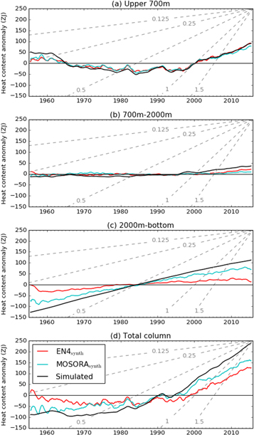
Figure 1. Simulated global OHC time series (ZJ, 1955–2015) for the following depth layers: (a) 0–700 m, (b) 700–2000 m, (c) 2000 m to bottom and (d) total column in EN4synth, MOSORAsynth, and the model 'truth'. Each time series is centred on the period 1955–2015 and smoothed with a 12 month running mean. Dashed grey lines show the equivalent heating rate calculated over the Earth's surface area for radiative fluxes of 0.125, 0.25, 0.5, 1 and 1.5 W m−2 as labelled.
Download figure:
Standard image High-resolution imageTable 1. Rates of global ocean heat content change (W m−2) over the period 1971–2010 in different depth layers expressed relative to Earth's surface area. The values in parentheses are the percentage by which each analysis underestimates (negative values) or overestimates (positive values) the model simulated trend (note that these percentages are calculated using data with higher precision than shown in the tables).
| Model 'truth' | EN4synth | MOSORAsynth | |
|---|---|---|---|
| 0–700 m | 0.12 | 0.10 (−19%) | 0.09 (−27%) |
| 700–2000 m | 0.06 | 0.02 (−76%) | 0.00 (−98%) |
| 2000 m to bottom | 0.25 | 0.06 (−76%) | 0.17 (−31%) |
| Total column | 0.44 | 0.18 (−60%) | 0.28 (−37%) |
Table 2. As table 1, but for the period 2006–2015.
| Model 'truth' | EN4synth | MOSORAsynth | |
|---|---|---|---|
| 0–700 m | 0.39 | 0.39 (+2%) | 0.32 (−16%) |
| 700–2000 m | 0.12 | 0.12 (+5%) | 0.06 (−52%) |
| 2000 m to bottom | 0.20 | −0.02 (−110%) | 0.12 (−39%) |
| Total column | 0.70 | 0.50 (−29%) | 0.50 (−30%) |
Time series for the 0–700 m layer are characterized by an initial decrease of OHC during the 1960s followed by a stronger increase since 1995. This depth range was sampled by XBT profiles for the period of interest, albeit with varying sampling density. Both mapping methods successfully reconstruct the variations in globally integrated OHC in the 0–700 m layer between 1955 and 2015, although the peak in the 1960s is underestimated. Some spurious monthly-to-interannual variability that is not seen in the model 'truth' is introduced in each analysis. For example, there are peaks in 0–700 m OHC in the mid-1970s and early 1980s that feature in both analyses, and are prominent in the total column OHC time series (figure 1(d)). This spurious variability appears to be less pronounced in the later part of the time series, likely due to improved observational coverage.
The 700–2000 m depth range is interesting as it is only since the introduction of Argo in the early 2000s that there has been systematic and near-global sampling of this layer (Roemmich et al 2015). Perhaps unsurprisingly, neither mapping method captures the trend in this layer prior to the Argo array reaching full maturity (figure 1(b); table 1); EN4synth and MOSORAsynth underestimate the trend by 76% and 98% respectively. Over the period 2006–2015, when the Argo array is close to the target number of floats, EN4synth appears to better capture the trend in this layer (5% overestimate). Over the same period, MOSORAsynth underestimates the magnitude of the trend in this layer by 52%.
The long-term global OHC change simulated by HadGEM3 is dominated by the layer below 2000 m (figures 1(c), (d)). This unrealistically large trend is likely the result of the ongoing model 'spin-up' or 'drift' described in section 2. While this deep signal is still useful for gaining insights into the ability of the mapping methods to recover the trend in this layer, we must be careful not to over-interpret the results. In particular, if the spatial pattern of drift is different to that associated with the forced climate response, the sampling characteristics needed to capture real-world signals will likely also be different. Nevertheless, both analyses capture a warming of the deepest layers but the limited number of observations at this depth mean that the magnitude of the trend is underestimated. Below 2000 m, EN4synth underestimates the 1971–2010 warming trend by 76%. The trend is better captured by MOSORAsynth (31% underestimate), which we attribute to the use of near-perfect model covariances (estimated from a different historical simulation of HadGEM3) that contain information about the spatial patterns of deep ocean drift.
A separation of OHC change into contributions from each hemisphere is shown in supplementary figure S1, available online at stacks.iop.org/ERL/14/084037/mmedia. As could be expected from differing historical observational coverage, the two analysis products capture the temporal variability in the northern hemisphere OHC more successfully than in the southern hemisphere, most obviously in the 0–700 m depth range before 1990 (supplementary figures S1(a), (b)). As seen in the global OHC, both analyses underestimate the deep warming trend in each hemisphere, but MOSORAsynth is able to capture a large fraction of the trend in the southern hemisphere (supplementary figure S1(f)).
To further explore the characteristics of the OHC trends and the ability of the analysis products to capture them, we examine the zonally integrated heating rate over the period 1971–2010 as a function of latitude (figure 2). Throughout the northern hemisphere, the latitudinal variation in the 0–700 m heating rate is well captured by both analyses. In the southern hemisphere there is a strong peak in warming around 50° S, which both analyses underestimate to a similar extent. There are contributions to this Southern Ocean warming peak from all depth layers considered, and the analyses underestimate its magnitude in each, such that in the total column the strong heating rate of around 5.5 W m−1 is significantly underestimated by both. From figure 2(a), it is clear that in the upper 700 m, the 1971–2010 heating rates are more successfully captured in the better-observed northern hemisphere than in the southern hemisphere. Figure 2(c) reveals that the sub-2000 m warming trend seen in figure 1(c) is characterised by a near-homogenous heating throughout a wide latitude range. Although both analyses underestimate this deep heating rate, MOSORAsynth captures it more successfully, likely due to its use of near-perfect covariances as discussed previously.

Figure 2. Zonally integrated trend in OHC (107 W m−1) over the period 1971–2010 as a function of latitude for EN4synth, MOSORAsynth and the model 'truth'. Results are shown for depth layers (a) 0–700 m, (b) 700–2000 m, (c) 2000 m to bottom and (d) total column.
Download figure:
Standard image High-resolution imageSpatial patterns in the 1971–2010 trends are examined in more detail for the uppermost and deepest layers in figure 3. Both analyses are able to capture the regions of warming and cooling that are seen in the model 'truth'. In the upper 700 m these include a cooling in the subpolar North Atlantic, tropical Pacific and the Pacific sector of the Southern Ocean, and a warming in the North Pacific, Arctic and most of the Atlantic and Southern Ocean. The deepest layer is characterised by a heat gain throughout most of the global ocean, with the largest magnitudes throughout most latitudes of the Atlantic, and a heat loss in the subpolar North Atlantic and in the Atlantic sector of the Southern Ocean. EN4synth and MOSORAsynth capture these spatial features well, but underestimate their magnitude in the regions of strongest trends, especially the upper-700 m Southern Ocean warming. They both significantly underestimate the trends throughout the deep ocean. The homogeneity of the deep warming signal suggests that the underestimation of the global OHC trends seen in figure 1 is due to the difficulty in reconstructing large-scale anomalies from very sparse observations (rather than systematic biases in the distribution of observations in sampling the underlying trends). Due at least in part to the near-perfect covariances used, MOSORAsynth is better able to recover the spatial structure and magnitude of the deep warming trends, but it is still severely hampered by poor observational sampling in the deep ocean.
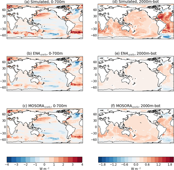
Figure 3. Global maps of 1971–2010 trends in OHC per unit area (W m−2) for the depth layers above 700 m (a)–(c) and below 2000 m (d)–(f). Results are shown for the simulated model 'truth' (a), (d), EN4synth (b), (e) and MOSORAsynth (c), (f).
Download figure:
Standard image High-resolution image3.2. Characterising errors in monthly-interannual variability
Having examined the analyses' reconstructions of global and hemispheric integrated quantities and long-term trends, we now explore the uncertainty in their estimates of monthly and annual temperature anomalies and monthly-interannual temporal variability. This is of particular relevance to their use in seasonal and decadal forecast initialisation and understanding climate variability. The ability of the mapping methods to reconstruct large scale patterns in annual mean fields is illustrated in figure 4. We present temperature anomalies for the year 1967 at 1000 m, although other years and depth levels reveal broadly similar characteristics. Despite the sparsity of the observations both mapping methods are able to reconstruct some of the large scale features, including warm anomalies in the North Atlantic, slightly warm conditions throughout most of the low to mid-latitude Pacific and Indian Oceans, and cool conditions in the Southern Ocean especially in the Atlantic sector. The structure of the anomalies is slightly closer to the model 'truth' in MOSORAsynth (for example around South Africa) demonstrating the potential benefit of near-perfect covariances, though the spatial correlation with the model 'truth' is only marginally higher: 0.52 for MOSORAsynth compared to 0.48 for EN4synth for this example year and depth. Time-mean spatial correlations for annual anomalies at 1000 m depth over the pre-Argo era (1955–2000) are 0.46 for MOSORAsynth and 0.42 for EN4synth; during the Argo era (post 2007) the correlations are substantially higher (0.80 and 0.78 for MOSORAsynth and EN4synth respectively).

Figure 4. Example reconstruction of the spatial pattern of temperature anomalies. Annual mean temperature anomalies (K) relative to 1955–2015 for 1967 at 1000 m are shown for (a) the original model simulation, taken as the 'truth' in this context, (b) synthetic observations (averaged onto the MOSORA grid), (c) the EN4synth analysis of synthetic observations and (d) the MOSORAsynth analysis of synthetic observations. The spatial correlation between the analysis and the model 'truth' is shown above panels (c) and (d).
Download figure:
Standard image High-resolution imageGeographical differences in the success with which the analyses capture temporal variability is examined by calculating the 1955–2015 mean absolute error in depth-integrated monthly temperature anomaly (supplementary figure S2). As could be anticipated, the analyses are less successful in capturing temporal variability in regions of high eddy activity and strong frontal gradients. In the upper 700 m, the largest errors in monthly anomalies are in western boundary current regions and around the Antarctic Circumpolar Current. The largest errors in the 2000 m bottom layer are found in regions close to sites of deep ocean ventilation, and include the North Atlantic and deep western boundary current regions. Conversely, errors are much smaller in regions of the deep ocean that have limited exchange with the surface ocean, such as much of the deep Pacific, since the variability in these regions is much smaller in magnitude.
We now further examine the ability of the analyses to capture temporal variability and how this varies over the decades as the real-world observing system evolved. Figure 5 shows the spatial pattern of the temporal correlation in depth-integrated temperature anomalies in various depth layers between EN4synth and the model 'truth' within three 10 year windows. These temporal windows have been chosen to compare results for the pre-XBT era (1956–1965), the XBT-era (1976–1985) and the Argo-era (2006–2015). Similar results are found for MOSORAsynth (supplementary figure S3). The time series at each grid point have been linearly detrended to avoid the influence of long-term drift on the correlation and the anomalies are calculated relative to a monthly climatology for each individual 10 year window. The highest correlations are found in the upper 700 m, and (with the exception of the sub-2000 m depth range in EN4synth) correlations are higher in the later decades as the observational density increases.
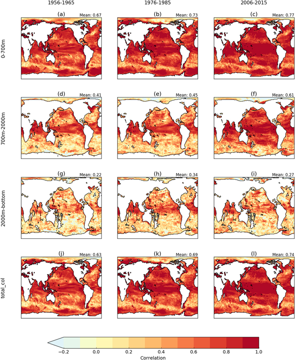
Figure 5. Temporal anomaly correlation in depth-integrated temperature between EN4synth and the original model simulation for the periods 1956–1965 (a), (d), (g), (j), 1976–1985 (b), (e), (h), (k) and 2006–2015 (c), (f), (i), (l). Monthly anomalies are calculated relative to a seasonally varying climatology derived for each 10 year period and then linearly detrended prior to calculation of correlations. The area-weighted spatial mean of the temporal correlation field is shown above each panel. Results are shown for 0–700 m (a)–(c), 700–2000 m (d)–(f), 2000 m to bottom (g)–(i), and the whole column (j)–(l).
Download figure:
Standard image High-resolution imageDespite the improved sampling from Argo during 2006–2015, the spatial pattern of temporal correlations for 0–700 m OHC (figures 5(a)–(c)) share similarities in all three periods. Patches of low correlation can still be seen in regions of high eddy activity, including the North Atlantic Current and much of the Southern Ocean, indicating that the observational density is not sufficient for the mapping methods to reproduce the limited mesoscale variability in the model 'truth' dataset. That EN4synth and MOSORAsynth are unable to recreate details of the eddy field is unsurprising given that the mapping methods were designed to reconstruct ocean anomalies with scales of hundreds to thousands of kilometres. Furthermore, even during the most recent decade Argo profiles have a typical spacing of 200–400 km, which is substantially larger than the first baroclinic Rossby radius of deformation in the mid- and high-latitudes. The low and/or negative correlations in the Arctic are indicative of the limited observation sampling in regions of shallow bathymetry and sea ice cover, which remains problematic even in the Argo era. Despite these limitations, the correlations are overwhelmingly positive in all three periods, suggesting that decadal climate predictions can feasibly be tested in re-forecasts covering the period since 1960 as proposed in the Decadal Climate Prediction Project (Boer et al 2016), albeit with caution when considering layers deeper than 700 m.
In the 700–2000 m layer (figures 5(d)–(f)), the effect of the introduction of the Argo array is more pronounced, with a large increase in correlation during 2006–2015 compared with the other two decades considered. The improvement is larger in the Pacific than the Atlantic. The spatial mean of the temporal correlation increases by 36% (EN4synth; figures 5(e)–(f)) and 49% (MOSORAsynth; supplementary figures S3(e)–(f)) between the 1976–85 and 2006–15 decades. Correlations in the layer below 2000 m (figures 5(g)–(i)) are generally very low, except in the tropics. The high correlation between the analysis and model 'truth' for the total column depth-integrated temperature anomalies reflects the dominance of upper ocean temperature variability on the monthly time scale.
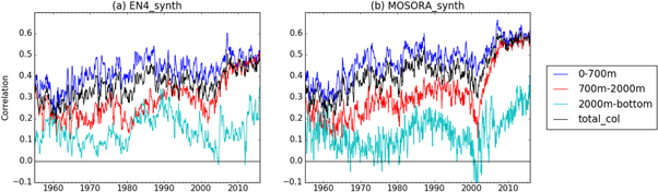
We now quantify the performance of the mapping techniques in recovering spatial patterns of depth-integrated temperature anomalies, and how this varies over time, by calculating spatial correlations for each month during the period 1955–2015 (figure 6). A large part of the time variations in spatial correlation will be due to changes in the observational network. As expected, the highest correlations are found in the upper 700 m layer and the lowest correlations in the layer deeper than 2000 m. The spatial correlations for total column integrated temperature are similar to correlations for the upper 700 m and reflect the dominance of the near-surface layers for column integrated temperature variability. The benefit of Argo is clearly evident as an increase in spatial correlations in both EN4synth and MOSORAsynth during the 2000s. This effect is most striking for the 700–2000 m layer, but is also evident in the upper 700 m and for the total column. For the period 2006–2015, there is a convergence of spatial correlations in the 0–700 m and 700–2000 m layers to about 0.5 in EN4synth and 0.6 in MOSORAsynth. The higher value for MOSORAsynth is likely a consequence of the near-perfect model covariances used, but illustrates the value of the method if global covariances can be adequately constrained. Although it was seen previously (figures 1–3) that MOSORAsynth is better able to capture the long-term deep ocean trend, EN4synth exhibits slightly higher spatial correlations for the deepest layer. Further analysis (not shown) suggests that this is because MOSORAsynth is penalised for attempting to recreate some degree of mesoscale structure, the details of which cannot be correct, whereas EN4synth creates smooth large-scale features where data is sparse. For similar reasons, in the deeper layers MOSORAsynth exhibits more high-frequency temporal variability in spatial correlation than EN4synth. In both analyses, all layers (particularly those in the deep ocean) exhibit decadal variations in the magnitude of spatial correlations. These variations are in phase in EN4synth and MOSORAsynth, which suggests they are a result of the evolving ocean-observing system and/or flow-dependent uncertainty in estimates of regional OHC that are modulated by decadal variability.
Figure 6. Monthly time series of global spatial pattern correlation between depth-integrated temperature anomalies in the model 'truth' and (a) EN4synth and (b) MOSORAsynth, for depth layers as labelled. The model 'truth' is first interpolated onto the grid of each analysis, and each dataset is linearly detrended and de-seasonalised.
Download figure:
Standard image High-resolution image
4. Summary and discussion
We have outlined a quantitative approach for assessing the accuracy of methods used to generate spatially complete analyses of ocean temperature from historical and present-day ocean observations. This approach is based on the use of 'synthetic profiles' from a known model 'truth' and has been applied to two statistical mapping procedures (those used in EN4 and MOSORA) in an idealised proof-of-concept study. By comparing the analyses derived from synthetic profiles with the model 'truth', the ability of each mapping method to reconstruct spatially integrated OHC change and regional OHC variability has been evaluated.
The time-evolution of the ocean observing system impacts the ability of both the EN4 and MOSORA methods to reconstruct simulated OHC anomalies in several foreseeable ways. Notably, the introduction of the Argo network of autonomous profiling floats during the early 2000s drives clear improvements in the ability of these methods to reconstruct OHC trends, variability, and spatial patterns in the 700–2000 m depth layer. At depths below 2000 m, both mapping methods underestimate the magnitude of the simulated ocean warming signal. The simulated deep ocean temperature trends are unrealistically large and a result of model drift, but the underestimation of the trends by the statistical mapping methods in this layer is consistent with the sparsity of historical observations (e.g. Durack et al 2014). The analyses appear to capture long-term heat content trends more successfully in the better-sampled northern hemisphere. They are both successful in reconstructing spatial patterns of long-term temperature trends in the upper ocean, but the magnitude of these trends is underestimated, particularly in the Southern Ocean. Furthermore, spurious interannual variability is introduced in estimates of global OHC time series in both EN4synth and MOSORAsynth that is not present in the model 'truth'. It is likely that this spurious variability is also due to the sparseness of historical observations, particularly since it is more prominent in the southern hemisphere and appears to reduce in magnitude in the later years. When looking at the spatial patterns of errors in OHC, we find that the largest mean absolute errors and lowest temporal correlations are concentrated in the regions of elevated mesoscale activity such as western boundary currents and frontal regions, which remain challenging to reconstruct in the Argo era. This result is consistent with a previous inter-comparison which found these areas to have the largest disagreement among products (Palmer et al 2017).
Despite the limitations of the historical observing network, and the idealised framework in which the mapping methods were performed, our results are encouraging for the validation of at least the upper 700 m global OHC time series. Our results also demonstrate that the historical observations, at least from around 1960 onwards, likely contain sufficient amounts of information such that potentially useful reconstructions of spatial temperature anomalies are feasible, especially in the upper ocean. This is encouraging for the development and assessment of initialised decadal climate predictions and the long-term monitoring of changes in OHC. Furthermore, there are clear benefits available from perfect covariances, motivating future research to improve the mapping techniques.
We note that this study is intended to demonstrate proof-of-concept in the method of using synthetic profiles to quantify errors in spatially mapped ocean analyses and, ultimately, OHC estimates. There are several ways in which the results are idealised and caution should be used when interpreting details of the results. The OHC trends and variability in the historically-forced simulation of HadGEM3 will be different to those in the real ocean, and we particularly note the influence of model drift on the deep ocean trends. Both mapping methods exploited perfect knowledge of the model's background temperature climatology, and near-perfect covariances were used to calculate MOSORAsynth, so the real world OHC estimates will be affected by these additional sources of uncertainty. To examine the performance of the mapping methods in a more realistic scenario, a background climatology calculated from the synthetic observations themselves (rather than the full model field) could be used, and covariances could be also calculated using the synthetic observations. The synthetic profiles technique could be used to test different methodological options for the calculation of global covariances, making it a useful tool for helping to improve the mapping methods.
The results of this proof-of-concept study are encouraging and the generic framework we have presented could easily be extended to different models, other statistical and/or dynamical mapping approaches, and other ocean variables (e.g. salinity, biogeochemical tracers). For example, data from high-resolution 'eddy-rich' ocean model simulations could provide important insights into the impacts of spatial representivity. Similarly, ensemble simulations that share the same forcing but different realizations of internal variability could be used to separate the impacts of flow-dependent uncertainties from the time-evolution of the ocean observing system. When extended to include additional mapping methods and use multiple model 'truth' datasets, this approach could be used to help quantify the uncertainty in real-world OHC estimates. Synthetic profile data sets thus have the potential to be a valuable tool for the oceanographic community and when used in a coordinated manner could provide powerful insights into the uncertainties associated with reconstructing the three-dimensional ocean state from historical and present-day observations.
Acknowledgments
This work was supported by the Met Office Hadley Centre Climate Programme funded by BEIS and Defra, and the European Union's Horizon 2020 research and innovation program under grant agreement No. 633211 (AtlantOS). We thank two anonymous reviewers for their insightful comments which greatly improved the manuscript.