

Abstract
We examine relationships between the start of rainy season (SOS) and sub-national grain (white maize) market price movements in five African countries. Our work is motivated by three factors: (a) some regions are seeing increasing volatility SOS timing; (b) SOS represents the first observable occurrence in the agricultural season and starts a chain reaction of decisions that influence planting, labor allocation, and harvest—all of which can have direct impacts on local food prices and availability; and (c) pre- and post-harvest price movements provide key insights into supply-and-demand issues related to food insecurity. We start by exploring a number of different SOS definitions using varying reference periods to define whether an SOS is 'on-time' or 'late'. We then compare how those different definitions perform in seasonal price forecasting models. Specifically, we examine if SOS indicators can predict price means over 6 and 9 month periods, or roughly the length of time from planting to market. We use different reference periods for defining 'early' versus 'late' seasonal starts based on the previous year's start date, or median start dates over the past 3, 5, and 10 year periods. We then compare the out-of-sample forecast performance of univariate time-series models (autoregressive integrated moving average (ARIMA)) with time-series (ARIMAX) models that include various SOS definitions as exogenous predictors. We find that using some form of SOS indicator (either an SOS anomaly or 1st month's rainfall anomaly) leads to increased predictive power when examining prices over a 6 months window. However, the results vary considerably by country. We find the strongest performance of SOS indicators in central Ethiopia, southern Kenya, and southern Somalia. We find less evidence in support of the use of SOS indicators for price forecasting in Malawi and Mozambique.
Export citation and abstract BibTeX RIS
1. Introduction
Sub-Saharan Africa suffers from chronic food insecurity, and much of the region is experiencing increasingly shorter and more volatile rainy seasons (Wainwright et al 2019). Grain production and grain prices in the region are heavily influenced by local environmental conditions, especially rainfall (Lobell and Field 2007, Brown and Kshirsagar 2015, Davenport and Funk 2015, Davenport et al 2018, 2019, Funk et al 2018, Nobre et al 2018). At the same time, grain price forecasting is a critical component of food-security analysis and famine early warning (Rubas et al 2006, Vogel and O'Brien 2006, Jayne and Rashid 2010, Naylor and Falcon 2010, Funk et al 2019). For example, high wholesale grain prices prior to harvest can signal lower-than-average production, and high consumer grain prices can exacerbate food insecurity (Barret and Mutambatsere 2005). Many poor households spend 60% or more of their income on food, and higher food prices typically lead to reduced food access.
A relatively new tool to food-security analysis and famine early warning are analyses based around the start of the rainy season (hereafter, SOS) (Shukla et al 2021). Analyses based on SOS offer an intriguing advance to famine early warning, as SOS represents the first observable agronomic indicator in the season and starts a chain reaction of decisions, such as when to plant (Marteau et al 2011) 1 , in-season resource allocation (Fink et al 2020), and when to harvest. These decisions can have direct impacts on local food availability. The SOS, both the amount of rainfall and when it arrives (relative to prior years), provides a key signal as to what the subsequent growing season and harvest will look like. In food-insecure areas dependent on regionally grown rainfed crops, SOS could potentially be a pivotal early indicator of food availability for the following year.
However, relatively little work has been done on the role that SOS indicators can play in forecasting. One recent paper (Shukla et al 2021) demonstrates the strong regional relationships between SOS and peak NDVI anomalies (an indicator frequently used as a proxy for grain production). Specifically, they find a large and statistically significant relationship in which late SOS is associated with decreased peak NDVI, indicating a relationship between late SOS and low plant productivity. This relationship is strongest in chronically food-insecure regions of east Africa. A recent conference presentation (currently a manuscript in-preparation) shows strong relationships between SOS and farmer planting decisions, indicating that SOS measures can be used to approximate planting dates when that data is unavailable (Krell et al 2019).
In this paper, we explore whether incorporating information on SOS 2 can improve seasonal price forecast accuracy. We start by exploring a number of different SOS definitions using varying reference periods to define whether an SOS is 'on-time' or 'late'. We compare how those different definitions perform in seasonal price forecasting models.
Specifically, we examine if SOS indicators can predict maize price means over 6 and 9 month periods, or roughly the length of time from planting to market. We use different reference periods for defining 'early' versus 'late' seasonal starts based on the previous year's start date, or median start dates over 3, 5, and 10 years before the current season. In this way, we attempt to frame what the best reference time period is for determining if onset of the rainy season is late or not. We then compare the out-of-sample forecast performance of univariate time-series (autoregressive integrated moving average (ARIMA)) models with time-series (ARIMAX) models that include various SOS definitions as exogenous predictors (X).
We use these results to identify markets and regions where SOS measurements can enhance maize price forecasts. These markets present a typology that analysts can use to identify markets that are responsive to SOS conditions. While there is rich literature on the use of environmental variables to predict grain prices in developing countries (Brown et al 2006, 2008, 2012, de Beurs and Brown 2013, Algieri 2014, Brown and Kshirsagar 2015, Davenport and Funk 2015, Peri 2017), to our knowledge, this is the first paper to explicitly use and test rainfall-based SOS measures as a price predictor.
2. Background and data
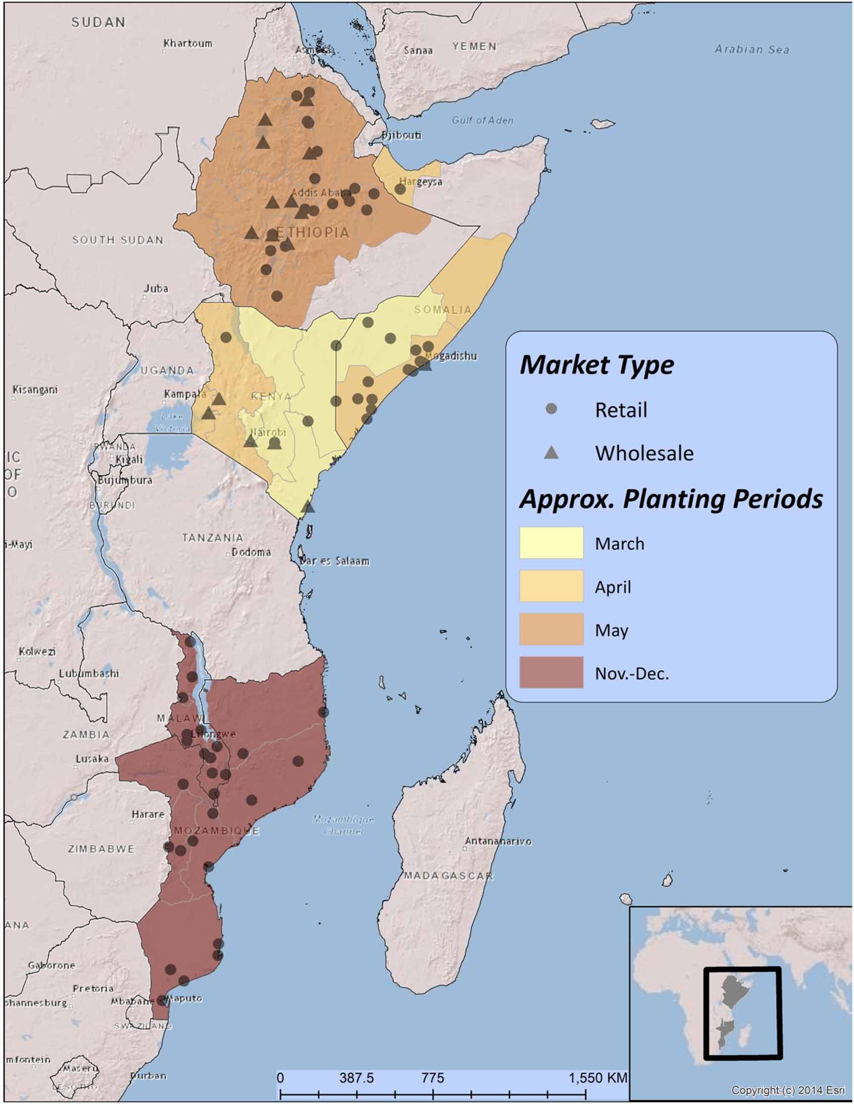
Our study focuses on several countries in eastern (Kenya, Somalia, and Ethiopia) and southern (Malawi and Mozambique) Africa. Figure 1 shows a map of the study area—the markets we examine and the approximate planting periods in the various regions. We focused our analysis on those markets in eastern and southern African countries with a minimum of 10 years' worth of maize (which is one of the major crops/food sources in this region) price data. The planting periods shown in figure 1 are from the GEOGLAM 3 Crop Calendars 4 and are approximations based on reviews of crop calendar data collected from international agencies, agricultural ministries, and expert knowledge (GEOGLAM 2021).

Figure 1. Map of study area, markets, and approximate planting periods. Basemap reproduced from ESRI (2012). Copyright (c) 2014 ESRI.
Download figure:
Standard image High-resolution image2.1. SOS definition
In this study, we focus on two aspects of the SOS: the timeliness (SOS anomaly) and the total amount of rainfall in the 1st month (1st month rainfall). This discussion focuses on the SOS metric; however, supplemental section S2 (available online at stacks.iop.org/ERL/16/084050/mmedia) provides an overview of seasonal rainfall history (wet and dry years) in the countries of interest.
To define the SOS, we use a threshold amount and distribution of rainfall received in three consecutive dekads 5 , as defined by the Centre Regional de Formation et d'Application en Agrométéorologie et Hydrologie Opérationnelle (AGRHYMET 1996). The AGRHYMET SOS definition is frequently used and evaluated in applied settings (Reason et al 2005, Tadross et al 2005, Rojas 2007, Funk and Budde 2009, Crespo et al 2011, Harrison et al 2011, Guan et al 2014, Ojo and Ilunga 2018, Shukla et al 2021) and is used to define SOS in the Water Requirement Satisfaction Index—a crop-weather analysis model commonly used by FEWS NET 6 for monitoring ongoing growing seasons (Verdin and Klaver 2002, Verdin et al 2005). Recent comparisons with field surveys also show this SOS metric to be an effective means for estimating farmer planting dates (Krell et al 2019).
The SOS metric is as follows: an SOS is established when there are at least 25 mm of rainfall in a dekad, followed by a total of at least 20 mm of precipitation in the following two consecutive dekads. If these rainfall thresholds are satisfied, the SOS is defined as the 1st dekad in that 3 dekad series. The SOS growing season window, the period in which we begin monitoring for rainfall to indicate a SOS, begins in February for east Africa, and in September for southern Africa 7 . The monitoring of rainfall begins before the estimated planting to capture early-season rainfall (SOS), and because farmers generally wait until after the first rains to begin planting. The SOS metric is calculated on a grid cell basis, using the Climate Hazards Center InfraRed Precipitation with Stations (CHIRPS 8 ) precipitation data set (Funk et al 2015), to attain gridded (0.1° latitude × 0.1° longitude) SOS for our years of interest (1981–2018).
SOS timeliness (anomalies) are then calculated by comparing a given year's SOS grid to a defined reference period. The varying reference periods included: the previous year and the median start dates over the past 3, 5, and 10 year periods. This process, and its application, are described in more detail in the following section 2.2. In addition to the timeliness of the SOS, total rainfall in the 1st month (3 dekads) is also used as a relative measure of the start to the rainy season in order to also explore the importance of early rainfall amount versus timing.
We match SOS and 1st month's rainfall to markets by taking the spatial averages of gridded surfaces in 100 km buffers surrounding each market location (shown in figure 1). We use 100 km because we do not know the exact centroids of the markets (the points correspond to populated areas) and want to ensure that they account for the entire region of surrounding buyers and sellers that might visit a given area 9 .
2.2. Using varying reference periods to define anomalies
After calculating spatial averages for each year and month, we convert each of our predictor variables (SOS and 1st month's precipitation) into climate anomalies (value in a given month differenced from a median calculated from prior years) prior to model fitting. The use of anomalies as predictors is standard practice when working with environmental variables, especially in a climate context, as they place the key variable in a context relative to spatial and seasonal averages. In this paper, we explore if the reference period used to define an anomaly impacts model performance. Specifically, we define anomalies over a 1, 3, 5, and 10 year rolling median (rm) and compare the predictive performance of these anomalies across models. For example, if the performance of an SOS indicator based on a 1 year anomaly notably outperforms a model based on a 10 year anomaly, this provides useful information for future predictive models. Formally, the SOS anomalies are defined by:

where SOS is the dekad of season start in y and N refers to the 1, 3, 5, and 10 year reference periods.
As mentioned above, we also fit predictive models that use early season rainfall anomalies (instead of SOS anomalies) using rainfall means defined over the same 1, 3, 5, and 10 year periods. In the models that use rainfall anomalies, we only use the 1st month in the season, (defined by the crop calendars in shown in figure 1). We do this to compare two different but overlapping potential SOS indicators: when the season starts and how much rain falls at the very beginning of the season. Ultimately, this could serve to assist analysts in defining the best reference period and SOS metric for what makes a late versus an on-time SOS.
2.3. Price data
We use monthly wholesale and retail nominal 10 white maize prices for 74 markets in Ethiopia, Kenya, Somalia, Malawi, and Mozambique 11 (figure 1). Data are collected, cleaned, and consolidated in the FEWS NET Data Warehouse, though not all data sets are publicly available at this time. All currencies were converted to USD per kilogram prior to model fitting. We only examine markets with ten or more years of continuous monthly price data. Since SOS events only happen once a season, we focus our analysis on seasonal price levels—specifically, monthly prices averaged over 6 and 9 month periods following approximate planting months (figure 1). This follows the goal of this paper in identifying how useful SOS indicators are in predicting seasonal price levels.
Figure 2 plots monthly mean maize prices (aggregated across markets) through the growing season. On the x-axis, '1' indicates approximate planting periods. For example, based on this figure, the planting period '1' might be March or April for eastern African countries and November for southern African countries. The colors indicate average prices (through the season) for years with a late versus an on-time season start. The figure suggests that late seasons tend to have higher prices, and these persist past the harvest periods. It should be noted that the highest levels of food insecurity often occur during the 'lean period', which falls within the rainy season, but before the harvest, i.e. around month three or four.
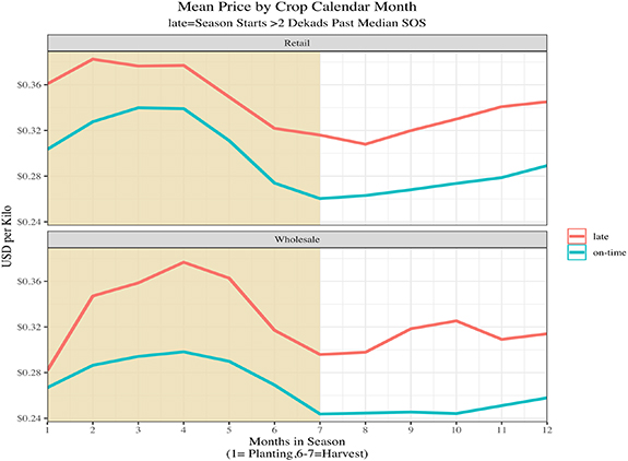
Figure 2. Mean white maize prices by crop calendar year during late and on-time years. The x-axis indicates the approximate month of planting (see figure 1). The red line shows mean prices during crop calendar months, when the SOS is late (>2 dekads) based on a rolling 10 years median. The blue line shows mean prices when SOS is early or on-time (⩽2 dekads).
Download figure:
Standard image High-resolution image3. Methods
Our baseline time-series model is a univariate (no exogenous predictors) ARIMA model,
where  is the time-series of observed prices averaged over either 6 or 9 months from planting, and the subscript t indexes years. The indicates potential differencing of the time-series, p is the order of lags,
  are the autoregressive parameters, q is the order of moving averages,
  are the moving average parameters, and
  are forecast errors from the prior periods. ARIMA (p,d,q) models are standard and frequently used methods for time-series analysis and forecasting (Hyndman and Khandakar 2008, Hyndman and Athanasopoulos 2018)
12
.
are forecast errors from the prior periods. ARIMA (p,d,q) models are standard and frequently used methods for time-series analysis and forecasting (Hyndman and Khandakar 2008, Hyndman and Athanasopoulos 2018)
12
.
We investigate if SOS can be used to enhance forecast accuracy of seasonal grain prices. We compare accuracy of forecasted price means over 6 and 9 month periods. We analyze forecasts made with univariate ARIMA models (using just historical price means), ARIMAX where the exogenous variable is an SOS anomaly, and ARIMAX models where the exogenous variable is the 1st month's precipitation anomaly.
Our basic workflow is as follows. For each set of market time-series, we do the following:
- (a)Fit univariate ARIMA (p,d,q) and ARIMAX (with an SOS measure as a predictor) models where the dependent variable is average price either 6 or 9 months from planting. Each market is initially fit on 5 years of data.
- (b)Repeat this process for each market using an expanding window cross-validation approach and record the forecast error. For example, we fit a model on 5 years of data and forecast price averages in year 6. We then fit a model on 6 years of data, forecast year 7, and repeat. The final column in table 1 shows the total number of forecasts—for each of the 9 methods we evaluate—stratified by country and market type.
- (c)The forecast errors for each series are averaged together to calculate one mean absolute percent error (MAPE) score for each market and method.
- (d)Finally, we compare forecast error across markets, forecast horizons (6 and 9 month means), methods (with and without an SOS measure), and lags (1, 3, 5, and 10 years rm) used to define anomalies.
Table 1. Market type (wholesale versus retail), number of markets of each type, min/max of years and number of observations, and the mean of the minimum and maximum SOS by country and market type. SOS numbers are dekadal (10 d) anomalies based on a 5 years rm, negative numbers indicate early start (in dekads), and positive numbers indicate late start. The price variables (mean min price, mean avg price, and mean max price) are seasonal price (in USD per kilo) minimums, means, and maximums averaged over the corresponding countries and market types. The final column 'no. of forecasts' shows the total number of out of sample forecasts done for each method we test (805 forecasts are made for each method).
| Country | Market type | No. of markets | Min year | Max year | Min N | Max N | Mean min SOS | Mean max SOS | Mean min price | Mean avg price | Mean max price | No. of forecasts |
|---|---|---|---|---|---|---|---|---|---|---|---|---|
| Ethiopia | Retail | 18 | 2006 | 2018 | 11 | 13 | −2 | 3 | 0.25 | 0.32 | 0.38 | 121 |
| Ethiopia | Wholesale | 10 | 2004 | 2018 | 15 | 15 | −2 | 2 | 0.2 | 0.26 | 0.31 | 90 |
| Kenya | Retail | 3 | 2000 | 2018 | 18 | 19 | −6 | 9 | 0.38 | 0.44 | 0.5 | 37 |
| Kenya | Wholesale | 5 | 2000 | 2018 | 10 | 19 | −2 | 4 | 0.25 | 0.3 | 0.35 | 57 |
| Somalia | Retail | 15 | 1995 | 2018 | 11 | 24 | −2 | 6 | 0.23 | 0.31 | 0.39 | 233 |
| Somalia | Wholesale | 1 | 1995 | 2018 | 24 | 24 | −3 | 8 | 0.21 | 0.29 | 0.38 | 18 |
| Malawi | Retail | 12 | 2002 | 2018 | 13 | 16 | −2 | 3 | 0.18 | 0.25 | 0.36 | 101 |
| Mozambique | Retail | 14 | 2002 | 2018 | 11 | 17 | −3 | 3 | 0.2 | 0.28 | 0.4 | 148 |
We evaluate forecast error using the MAPE. We analyze the MAPE in several ways. To provide an overview of performance, we use Nemenyi/MCB (multiple comparison with best) tests (Koning et al 2005, Demšar 2006). These tests were pioneered to perform a post-hoc analysis of the methods used in the M3 13 forecasting competition. The basic process is to rank the forecast performances of each method on each time-series, and then estimate median ranks of performance along with confidence intervals for those ranks. Intuitively, this is similar to doing a regression on the ranks of the MAPE scores using dummy variables for each modeling approach and then comparing the estimated coefficients for each model.
However, we do not want to rest our analysis solely on significance tests (Wasserstein and Lazar 2016, Amrhein et al 2019, Wasserstein et al 2019). We are more interested in regional variation in the value of SOS predictors and identifying areas where SOS indicators add value to food-security analysis. Therefore, we also present several descriptive measures to summarize model performance. We plot the performance of each SOS-based model, relative to the univariate model, across countries (and season types) to identify any emerging patterns. Finally, we map the markets where SOS-based indicators consistently outperform univariate models, regardless of the indicator used.
4. Results
4.1. Nemenyi tests comparing ranks of model accuracy scores
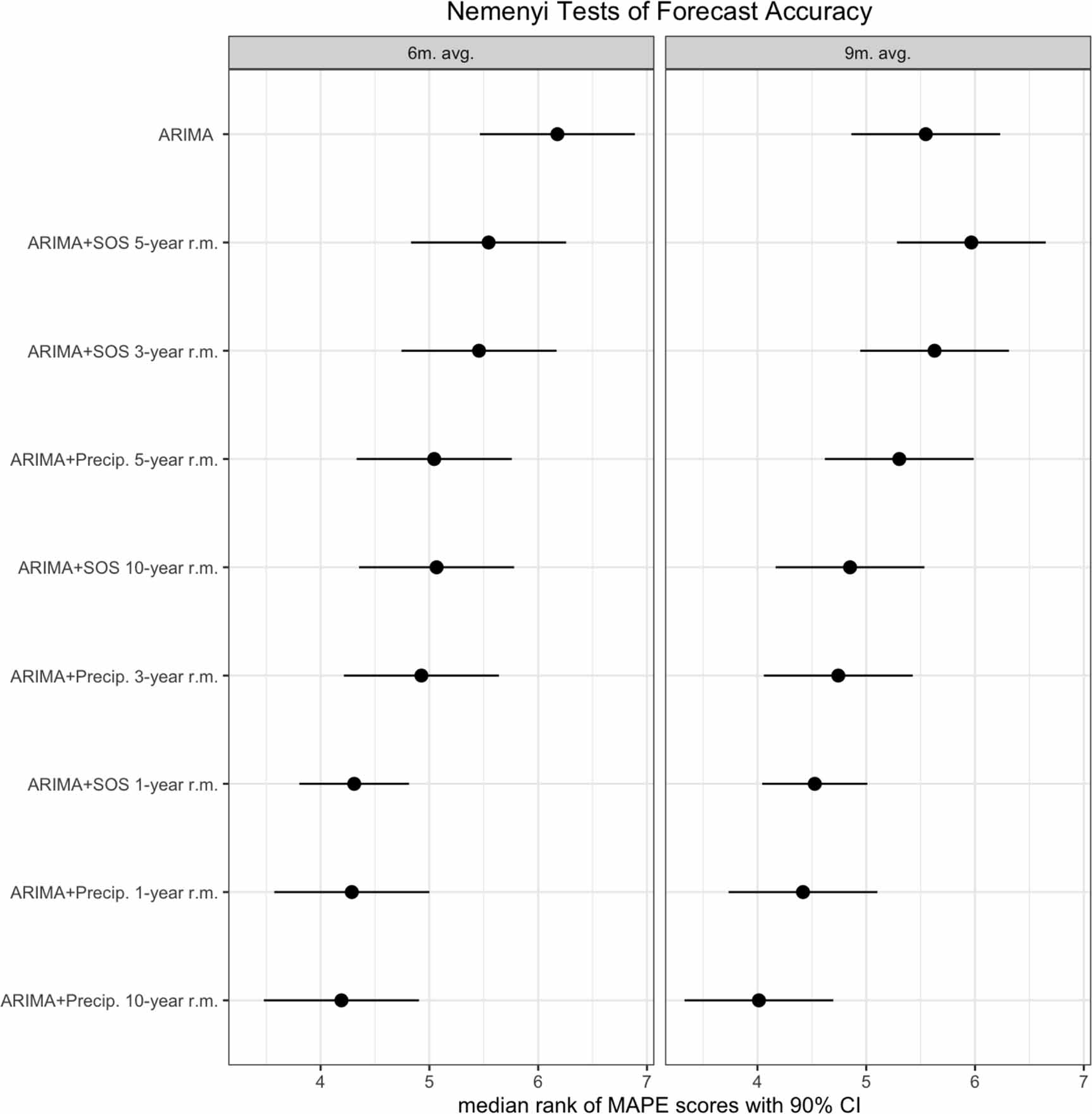
We first present an overall summary of how the different models performed. Figure 3 shows estimated MAPE ranks and 90% confidence intervals resulting from the Nemenyi tests (nine methods evaluated across 74 markets for a total of 666 MAPE scores). For the 6 months time period, we see that the univariate model, on average, performs worse than all others, and adding SOS or 1st month's precipitation anomaly as a predictor results in higher forecast skill. In the 9 months period, the univariate ARIMA model is 2nd to last, outperforming the 5 years lag-based SOS model. The models based on 1 and 10 year anomalies all perform best in either period. We suspect the increased performance of SOS in the 6 months forecast period is due to the fact that, as observations get farther from the SOS, more information and events outside of initial conditions could start influencing prices, diminishing the importance of initial conditions. In the middle of the growing season, grain from the previous season is being consumed, food availability is low, and prices tend to increase (figure 2). A poor start to the season may contribute to a perceived increase in risk and food prices.
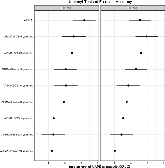
Figure 3. Nemenyi tests of forecast accuracy based on nine methods where each method is evaluated on 74 markets. Median ranks and 90% confidence intervals outputted from Nemenyi tests. Lower values on the x-axis (higher ranks) indicate better performance. Different forecasting approaches are shown on y-axis, where rm indicates the period of rolling median used to define the lag. The univariate ARIMA models have the highest (worst) MAPE scores for the 6 months forecast horizon but do slightly better in the 9 months horizon.
Download figure:
Standard image High-resolution image4.2. Results by country
Figure 4 shows results by country (aggregated across market). The x-axis shows the difference in MAPE scores between SOS/precipitation-based models and the univariate ARIMA model. Points that fall to the left of the vertical line indicate that a given model outperformed the univariate model. Colors indicate whether the prediction was made in a normal/early year versus a late start year (for a given market area).
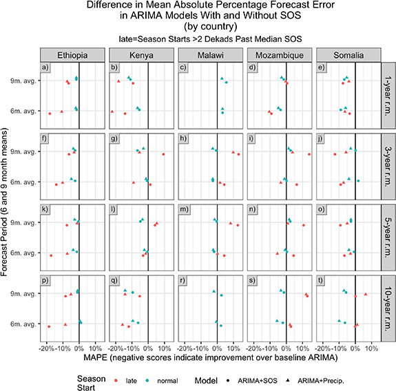
Figure 4. Difference in MAPE scores for each market, forecast period, and lag definition. The x-axis shows the difference between forecast accuracy of a model that uses some measure of SOS anomaly and a univariate model. Values below (to the left of) the vertical line indicate where an SOS-based measure provides more accurate forecasts than a univariate ARIMA model. This plot shows the difference in out-of-sample MAPE scores for each market, averaged across all markets with separate colors for late versus normal/early years and separate symbols for the type of predictor used. The columns are for each country and the rows are for each rm period used to define the seasonal anomaly. Each point is vertically offset in order to avoid plotting points on top of each other.
Download figure:
Standard image High-resolution imageIn general, we see the most support for SOS indicators improving forecast performance in Ethiopia and Kenya, with the strongest results for the 1 and 10 years based anomalies and, as expected, stronger performance when the season start is defined as late. In Somalia, these same results hold for the shorter periods (1, 3, or 5 years), but not for the 10 year period. In contrast, results are more ambiguous for Malawi and Mozambique, where the indicators often do not outperform the basic model even in late years. In general, we do not see large performance differences between the different types of SOS indicators (SOS anomaly or the 1st month's precipitation), although the SOS anomaly-based model has consistently shown the best performance in Ethiopia during the 6 months forecast window.
4.3. Results by market
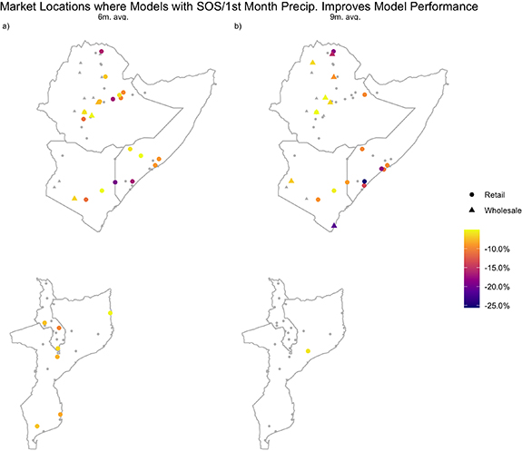
Finally, we present results at the market level. Figure 5 shows markets where price models with SOS indicators beat the univariate models by more than 5% (regardless of lag type or indicator used). The purpose here is to identify markets where some form of SOS indicator can improve early season price forecast performance. Shapes indicate market type (wholesale versus retail), and darker colors indicate the strength of the SOS-based ARIMA model against the univariate model. Grey points are markets where SOS indicators do not increase forecast performance. In general, we see that SOS indicators primarily improve forecast performance in central Ethiopia, southern Kenya, and southern Somalia. With some exceptions, the spatial distribution of the successful SOS models aligns with drier, more drought-prone eastern areas (see supplemental figure S2). These regions have shorter seasons and less opportunity to recover from a delayed onset. There are only a few markets in Malawi and Mozambique, where SOS indicators routinely increase forecast performance.
Figure 5. Map showing markets where the average MAPE score, regardless of model type, is 5% or lower than the univariate ARIMA model. Lower scores indicate better performance. The figure shows markets where SOS indicators consistently produce better forecasts. Markets where this is not the case are shown in grey.
Download figure:
Standard image High-resolution image
5. Discussion and conclusion
We find that using some form of SOS indicator (either an SOS anomaly or 1st month's rainfall anomaly) leads to increased predictive power when examining prices over a 6 months window. However, the results vary considerably by country. We find the strongest performance of SOS indicators in central Ethiopia, southern Kenya, and southern Somalia. We find less evidence for the use of SOS indicators for price forecasting in Malawi and Mozambique. These findings support other research suggesting that, within sub-Saharan Africa, the relationship with SOS and food-security measures is strongest in east African countries (Shukla et al 2021).
The evidence demonstrating that using a specific reference period (1, 3, 5, or 10 years) to define a season anomaly will increase performance is less conclusive. While the MCB tests suggest that all anomaly definitions tend to outperform univariate models, there is not an obvious pattern, as both the 1 and 10 years based anomalies were ranked as the overall best indicators, and there was substantial heterogeneity of these results across regions. One explanation for the performance of the 1 and 10 year anomalies is that a late start or low rainfall based on a 10 years anomaly may signify a substantial drought, while the 1 year anomaly simply reflects a cognitive bias towards the most recent events (short-term memory).
The relative insensitivity of the reference period may be also related to the year-to-year stationarity of the African monsoon systems. These systems move south and north in response to latitudinal variations in insolation and shifts in the Indian Ocean's complex annual wind patterns (Funk et al 2016). Given this strong climatological cycle, the baseline 1, 3, 5, and 10 year values used to calculate the anomalies could be quite similar.
This same feature—the strong phase locking of the seasonal cycle, can also help to explain the value of SOS indicators. In drier areas of central-eastern East Africa, the end of the rainy season is quite fixed, so a slow onset is an effective harbinger of higher prices. In Malawi and central-northern Mozambique, cessation of the monsoon season is less distinct, and this may help account for the weaker SOS relationships.
We also suspect that the use of historical references to define what is a 'normal' season likely varies significantly across market-sheds, buyers, sellers, and even farmers; this heterogeneity creates a more muddled picture when aggregated across countries and years. For example, the 10 year indicators did not perform as well in Somalia, which may reflect the long period of civil conflict in that country (e.g. other factors, such as conflict, pests, and disease can inhibit the influence of long-term seasonal anomalies on market prices). It is possible that this heterogeneity in response to seasonal trends, along with uneven patterns of spatial price transmission in the region (Brown et al 2012, Ansah et al 2014), also explains why the results are less spatially clustered than we would expect 14 . A final source of uncertainty is the lack of explicit knowledge of planting dates. While we have preliminary evidence that planting dates generally coincide with SOS (Krell et al 2019), and we have general knowledge of regional crop calendars (GEOGLAM 2021), we also know that the timing of planting is driven by a host of factors and that these may vary by year across regions. This is one of the reasons why we focus on aggregate price means and limit our results to markets with at least 10 years' worth of price data—so that our conclusions focus on price levels across seasons and regions rather than a specific market, month, or year. We anticipate that the heterogeneity of individual farmer's or market's responses to SOS could be better teased out with future survey data or field experiments. However, we are confident in asserting that, when making forecasts, the specific reference value is less important than simply including some measure of early season anomaly, particularly in east African countries.
This has important potential applications in terms of price forecasting and intervention planning. Our results imply that late onset of the rainy season can impact market behavior quickly, months before harvest (figure 2). If price variations are driven by expectations, rather than actual physical grain deficits, then that can help explain the rapid, and potentially deadly, jump in prices seen in Kenya, Somalia, and Ethiopia during the drought years 2011 and 2017 (Funk et al 2018) 15 . These price spikes occurred in the middle of the growing season, long before harvest. These rapid and dangerous price shocks require rapid and effective responses, which can be supported by staged early warning systems (Funk et al 2018).
In regards to future research opportunities, there are several intriguing avenues. The first might be to investigate explicit monthly price movements, not seasonal averages, as we do here. Our goal in this paper is to provide a general sense of the usefulness of SOS indicators; however, as the results suggest, there is considerable heterogeneity in market price behavior, and thus, a more finely detailed exploration at the monthly and individual market level might provide more insight as to why certain markets do or do not respond to seasonal start signals. A finer-grained analysis might also explore alternate crops, a wider range of forecast windows, and a more detailed examination of wholesale and retail level prices. We are also interested in exploring SOS definitions with finer temporal resolution (perhaps at the daily level) to examine the extent that this might influence very near-term price movements and volatility. Finally, there is an emerging set of Earth observation products that can be used to forecast SOS which, if quantitatively linked to food-security outcomes, could also be promising for developing extended seasonal outlooks.
Acknowledgments
An early version of this paper was presented (as a poster) at the 2019 AGU meetings in San Francisco. Juliet Way-Henthorne served as an in-house editor for several versions of this paper. Our sincere thank you to Sonja Perakis and the FEWS NET data and price teams for their assistance with obtaining and understanding the data and for their insightful feedback on numerous versions this manuscript. Funding for this research came from several sources. Including USAID (Award # 72DFFP19CA00001), the NASA SERVIR program (Award # 80NSSC20K0159), and the DAPRA World Modelers program (Award # W911NF-18-1-0018). Any opinions, findings, and conclusions or recommendations expressed in this material are those of the author(s) and do not necessarily reflect the position or the policy of the Government or the Prime Contract and no such official endorsement by either should be inferred.
Finally we thank two anonymous reviewers for their time and critical feedback.
Data availability statement
The data generated and/or analyzed during the current study are not publicly available for legal/ethical reasons but are available from the corresponding author on reasonable request.
Footnotes
- 1
We present a brief literature review of rainy season onset and farmer planting decision in supplemental S2.
- 2
Defined by one 10 d period with 25 mm of rainfall followed by two 10 d periods totaling 20 mm of rainfall. See section 2.1.
- 3
Group on Earth Observations Global Agricultural Monitoring Initiative.
- 4
- 5
Dekads are a common accumulation period within the agriculture monitoring community. The 1st and 2nd dekad of a month will contain 10 d, and the 3rd dekad will contain the rest of the days of the month (8–11 d) (WMO 1992). There are 36 dekads in a year.
- 6
Famine Early Warning Systems Network: https://fews.net/.
- 7
The monitoring period for these seasons ends in August for east Africa and March for Southern Africa. These windows are particularly important in areas, such as east Africa, in which there is a mixture of unimodal and bimodal rainy seasons (more than one growing season), and/or one of those seasons cross the calendar year.
- 8
Supplemental section S5 contains a detailed description of why we use the CHIRPS dataset for this analysis.
- 9
Our analysis includes both wholesale (sellers) and retail (buyers) and we want to account for as wide of activity space for both of types of market participants. Because our study areas include a variety of livelihood types, including agriculturalists, pastoralists, and agropastoralists, we want to encompass the seasonal activity spaces of all of these livelihood types. Of these livelihood types pastoralists tend to have the widest activity space and also tend to be the most food insecure and dependent on retail grain markets to meet their caloric requirements. While it is difficult to precisely identify the market-shed based on an individual centroid, the 100 km distance has been used in other studies of pastoralist (Grace and Davenport 2021), and is based on a review of movement and activity patterns of pastoral and agropastoral livelihood types in sub-Saharan Africa (Turner and Hiernaux 2002, Adriansen and Nielsen 2005, Adriansen 2008, Turner and Schlecht 2019).
- 10
We use nominal prices as it is difficult to impossible to find regional deflaters that can accurately correct for the widely varying costs of living in African countries, especially for remote rural environments. Operational forecasts in the region are generally made on nominal prices for this reason. We do our best to accommodate inflation/deflation empirically by fitting on first differences and including trend terms.
- 11
We chose these countries because they have historically experienced chronic food insecurity and drought, are among countries where price forecasts are used to support famine early warning, and have a number of markets with ten or more years of continuous monthly price data.
- 12
We use ARIMA models because they have a long and established history in both time series analysis and forecasting (Tsay 2000, Box et al 2015). Along with exponential smoothing (ETS), ARIMA models are the most popular and widely employed method for time series forecasting (Hyndman and Athanasopoulos 2018). While the two model types, ARIMA and ETS, broadly overlap, there are special instances of each that are not found in the other. However, we choose ARIMA models for this paper because it is easier to include external regressors (our main goal of this paper), the format we use—wherein we fit an ARIMA model to the residuals of a linear regression—can easily be compared across model fits and is extremely computationally efficient (we fit about 805 models for each method we evaluate). Finally we are able to fit all models using the auto.arima() function in R, which is specifically designed for this type of benchmarking (Hyndman and Khandakar 2008).
- 13
The M-Competitions are a series (M1, M2, M3, M4, M5) of forecasting competitions coordinated by Dr Spyros Makridakis and the International Institute of Forecasters. The purpose of the competitions is to evaluate both established and novel forecasting methods with a series of benchmark datasets. More information can be found here: https://forecasters.org/resources/time-series-data/.
- 14
In general, prior research has shown that sub-national markets in eastern and southern Africa are primarily influenced by a mix of local and regional influences. However they are not immune to very large exogenous shocks and prices in the bigger urban areas and major ports can be follow leads from the global cereals price indices (Brown et al 2012, Brown and Kshirsagar 2015).
- 15
For a more detailed analysis of price activity during this period (2011 and 2017) see figures 9 and 10 in Funk et al (2018). Available at: www.usaid.gov/sites/default/files/documents/1867/Kenya_Report_-_Full_Compliant.PDF.