
Abstract
No-broadcasting theorem is one of the most fundamental results in quantum information theory; it guarantees that the simplest attacks on any quantum protocol, based on eavesdropping and copying of quantum information, are impossible. Due to the fundamental importance of the no-broadcasting theorem, it is essential to understand the exact boundaries of this limitation. We generalize the standard definition of broadcasting by restricting the set of states which we want to broadcast and restricting the sets of measurements which we use to test the broadcasting. We show that in some of the investigated cases broadcasting is equivalent to commutativity, while in other cases commutativity is not necessary.
Export citation and abstract BibTeX RIS

Original content from this work may be used under the terms of the Creative Commons Attribution 4.0 license. Any further distribution of this work must maintain attribution to the author(s) and the title of the work, journal citation and DOI.
1. Introduction
The no-cloning theorem is perhaps the most famous limitation in quantum information processing. The impossibility to duplicate an unknown quantum state makes a fundamental difference between classical and quantum information processing. The no-cloning theorem is nowadays seen not only as an obstacle but a fact that enables e.g. secure communication protocols. Namely, since an unknown quantum state cannot be perfectly duplicated it follows that a potential eavesdropper on a quantum communication channel cannot capture messages without being detected. The no-cloning theorem is not an isolated feature of quantum theory but links to other impossibility statements such as the no-information-without-disturbance theorem and the non-existence of joint measurement for arbitrary pairs of measurements [1]. In that perspective, the violation of Bell inequalities can be seen as an experimental proof of the no-cloning theorem.
Later, an important distinction between cloning and broadcasting was made [2] and in the present work we concentrate on the latter concept, hence we recall their difference. A (hypothetical) perfect cloning device takes an unknown pure state ρ as an input and gives a composite system in a joint state  as an output. Even in a classical theory this condition cannot hold for all mixed states, therefore it makes more sense to pose it only for pure quantum states. In fact, the originally presented version of the no-cloning theorem formulates cloning for pure states and derives a contradiction from their superposition structure [3]. The defining condition for a perfect broadcasting device is weaker than cloning; it is only required that the output is a joint state ω of a bipartite system that has the duplicate of the initial state ρ as its both marginal states, i.e. the partial traces of ω are
 ![$\mathrm{tr}_{1}[\omega] = \mathrm{tr}_{2}[\omega] = \rho$](https://content.cld.iop.org/journals/1751-8121/56/13/135301/revision4/aacbc5bieqn2.gif) . The broadcasting condition captures the essence of the possibility to duplicate classical information as in a classical theory; the perfect cloning device for pure states is also a perfect broadcasting device that broadcasts all classical states, pure and mixed. In quantum theory the impossibility of universal and perfect broadcasting follows from the no-cloning theorem. This is due to the fact that a joint state with pure marginal states is necessarily a product state, hence for pure states broadcasting is the same as cloning. Therefore, taken only as categorical no-go statements, the no-cloning theorem and the no-broadcasting theorem are equivalent. We emphasize that the previous statements and also all the later developments in this work assume that there is one input copy. If there are more input copies, then no-cloning and no-broadcasting become separated and broadcasting of qubit states is, in fact, possible if there are four or more input copies available [4, 5].
. The broadcasting condition captures the essence of the possibility to duplicate classical information as in a classical theory; the perfect cloning device for pure states is also a perfect broadcasting device that broadcasts all classical states, pure and mixed. In quantum theory the impossibility of universal and perfect broadcasting follows from the no-cloning theorem. This is due to the fact that a joint state with pure marginal states is necessarily a product state, hence for pure states broadcasting is the same as cloning. Therefore, taken only as categorical no-go statements, the no-cloning theorem and the no-broadcasting theorem are equivalent. We emphasize that the previous statements and also all the later developments in this work assume that there is one input copy. If there are more input copies, then no-cloning and no-broadcasting become separated and broadcasting of qubit states is, in fact, possible if there are four or more input copies available [4, 5].
The separation between cloning and broadcasting becomes relevant when one considers approximate, non-universal or otherwise imperfect scenarios. The underlying theme is to find and characterize possible quantum devices that function as a cloning or broadcasting device in some approximate or limited manner. The sole no-go statement does not prevent the existence of a device with arbitrarily small nonzero deviation from the hypothetical cloning or broadcasting device. Since the existence of such an almost perfect device would evidently ruin the essence and practical consequences of the no-go theorems, this topic is important and various approximate scenarios have been exhaustively studied earlier [6, 7]. In approximate scenarios the distinction between cloning and broadcasting is not sharp as an actual device can be compared to both of these hypothetical devices and it simulates them imperfectly. Roughly speaking, if the aim is optimal approximate broadcasting, then the quality of output states is tested on the individual subsystems and no attention is paid to their joint state. In contrast to approximate scenarios, one can consider perfectly accurate but non-universal cloning or broadcasting devices, meaning that the input state is not completely arbitrary but belongs to some known subset of states. In this case the distinction between cloning and broadcasting is clear since the performance of the device is required to be perfectly that of the hypothetical device, just not on all states. It has been shown that a set of quantum states that can be broadcasted with a single quantum channel is contained in the simplex generated by a set of distinguishable states. In other words, maximal subsets of states that can be broadcasted are replicas of classical state spaces in the given quantum state space.
In the current work we generalize the setting of accurate but limited broadcasting. We formulate the concept of a broadcasting test, where the capability of a quantum channel to broadcast is tested with a setup consisting of some specified test states and test measurements. This formulation covers several interesting scenarios as special cases, some of which have been investigated earlier and some new arising naturally from the introduced framework. We prove that the defining condition of a broadcasting test reduces to a mathematical condition on factorization maps, determined by the corresponding test measurements. The derived condition on factorization maps avoids irrelevant details and provides tools to study any given broadcasting test. Further, the formulation of a broadcasting test in terms of factorization maps leads to a new viewpoint, where broadcasting can be seen as a certain kind of congruency relation on quantum channels. We prove that this relation is strictly stronger than the compatibility relation on quantum channels. In the final section we will study broadcasting in two specific cases: when the sets of measurements used to test the broadcasting are restricted and when the set of states and set of measurements on one side are restricted. We show that in all cases commutativity is sufficient for broadcasting, but, surprisingly, we also show that commutativity is strictly not necessary by constructing concrete examples of scenarios which are broadcastable, but not commutative. This complements the earlier result on broadcastable set of states where commutativity was often shown to be necessary. The general concept of a broadcasting test allows to study intermediate cases, where limitations are both of states and measurements.
2. Broadcasting tests
By a quantum channel we mean a completely positive and trace preserving linear map from a quantum state space to another quantum state space. These are the physically realizable input-output processes. Let us consider a scenario where a quantum channel  is planned to be used to broadcast an unknown state to two parties. Here
  is a fixed state space of d-dimensional quantum system. Generally, a channel from
  to
to  (or more generally to
  ) is called a broadcasting channel, irrespective of its action. Here we use
  to denote the tensor product of quantum state spaces,
  is the state space consisting of density matrices on the tensor product of the underlying Hilbert spaces. The broadcasting condition is

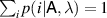
and due to the no-broadcasting theorem Λ cannot satisfy this for all states ρ. However, it may work like that in some limited setting. To test the functioning of Λ, we insert some test states as inputs and perform some measurements on the output states. The test states and measurements may be completely up to our choice, or they may be determined by some constrains e.g. of a communication scenario. In any case, we assume that the test states and measurements, although arbitrary, are fully known. A measurement is mathematically described as a positive operator valued measure (POVM), i.e. for each possible measurement outcome i is assigned a positive operator  and
and  . The measurement outcome distribution in a state ρ is given as
 ![$\mathsf{A}_i(\rho): = \mathrm{tr}\left[\rho \mathsf{A}_i\right]$](https://content.cld.iop.org/journals/1751-8121/56/13/135301/revision4/aacbc5bieqn12.gif) for all i and we will use
for all i and we will use  to denote the set of all measurements on
  .
.
If a state ρ is inserted to a broadcasting channel Λ and  and
and  are measurements on the output sides, then Λ functions in the intended way if the measurement outcome probabilities are the same for the input state ρ and for the transformed states
 ![$\mathrm{tr}_{2}[\Lambda(\rho)]$](https://content.cld.iop.org/journals/1751-8121/56/13/135301/revision4/aacbc5bieqn17.gif) and
and ![$\mathrm{tr}_{1}[\Lambda(\rho)]$](https://content.cld.iop.org/journals/1751-8121/56/13/135301/revision4/aacbc5bieqn18.gif) , i.e.
, i.e. ![$\mathsf{A}(\mathrm{tr}_{2}[\Lambda(\rho)]) = \mathsf{A}(\rho)$](https://content.cld.iop.org/journals/1751-8121/56/13/135301/revision4/aacbc5bieqn19.gif) and
and ![$\mathsf{B}(\mathrm{tr}_{1}[\Lambda(\rho)]) = \mathsf{B}(\rho)$](https://content.cld.iop.org/journals/1751-8121/56/13/135301/revision4/aacbc5bieqn20.gif) . This motivates the following definitions, illustrated in figure 1.
. This motivates the following definitions, illustrated in figure 1.
Definition 1. A broadcasting test is a triple  , where
  is a collection of tests states and
  are collections of test measurements. We say that a channel
  passes the broadcasting test
 if
if


for all  ,
,  and
and  . If there exists a channel Λ that passes a broadcasting test
  , then we say that the triple
  is broadcastable.

Figure 1. (a), (b) In a broadcasting test some chosen test states are produced with a preparator (green device), inserted to a broadcasting channel (gray device) and measurements (blue and red devices) are then performed on the two output systems. (c) The measurement outcome distributions are compared to the situation where the same measurements are performed independently. If these two situations cannot be differentiated, then the channel passes the broadcasting test.
Download figure:
Standard image High-resolution imageClearly, universal perfect broadcasting corresponds to the choices  and
and  and by the no-broadcasting theorem there is no channel that would pass the broadcasting test
  . The question is then to find the conditions when a triple
  is broadcastable. It is instructive to separate the following special cases:
- (a)Broadcasting of a subset of states. In this case test measurements are arbitrary but test states are from some limited subset of states, i.e.
 , . The conditions (2) and (3) can then be written as equation (1). It is customary to say that a subset of states is broadcastable when is broadcastable in the sense of definition 1. It has been proven in [8] that this is the case if and only if lies in a simplex generated by jointly distinguishable states. For instance, orthogonal pure states are distinguishable and hence a subset consisting of their convex mixtures is broadcastable.
 - (b)Broadcasting of a subset of measurements. This is the analog of the previous case, but now test states are arbitrary while test measurements are limited, i.e., . We also say that a subset is broadcastable when is broadcastable in the sense of definition 1. In the case of consisting of two measurements this reduces to the broadcastability relation studied in [9], where it was introduced as a strong form of compatibility and broadcastable pairs of qubit measurements were characterized. We present a full characterization of broadcastable sets of measurements in section 5, we show that in this case commutativity is sufficient but not necessary for broadcasting.
- (c)One-side broadcasting of subsets of measurements. When thinking about the previous scenario, there is no need for the subsets and to be identical as we can perform different kind of measurements on the two outputs. In the case of pairs of measurements this was called one-side broadcasting in [9] and it was shown that two qubit measurements are one-side broadcastable if and only if they are mutually commuting. We prove in section 5 that mutual commutativity is sufficient but not necessary in general.
- (d)Perfect transmission of a subset of states. If and , then the test states are perfectly transmitted to the -side. This scenario is more general than broadcasting of subsets of states since we may have , meaning that on the -side we make only a partial test. The scenario can correspond e.g. to eavesdropping, where an eavesdropper does not want to leave any traces from the intervenience. We present a characterization of broadcastable test states and test measurement in section 5, we show that in this case commutativity is necessary for broadcasting.


3. Reformulation of broadcasting tests
We begin this section with a simple observation. The equations (2) and (3) are linear in ρ,  and
and  . Therefore, if a channel Λ passes a broadcasting test
  , then it also passes the broadcasting test for all states in
  and all measurements in
  and
and  . Here
  denotes the linear span of a set X.
In the following we present a mathematically equivalent form of broadcasting tests. To do this, we introduce an equivalence relation that partitions the state space according to a particular test. Firstly, we say that a measurement  distinguishes two states ρ and σ if
  , meaning that the measurement outcome distributions for these states are different. We further say that a subset
  distinguishes two states ρ and σ if
  for some
  . For
. For  and
and  , we denote
  and say that ρ and σ are
 -equivalent if
  for all
  . Hence, two states are deemed
  -equivalent if no measurement in
  can distinguish between them.
A collection  is called informationally complete if it distinguishes all pairs of states. If
  is informationally complete, then clearly
  is broadcastable if and only if
  is broadcastable. In other words, if we would use informationally complete subsets of measurements in both output sides, then we have the state broadcasting scenario (case (b) in section 2).
For any  , we denote the equivalence classes in the equivalence relation
  as
as

We further denote ![$\mathcal{T}_{\mathcal{A}} = \{[\rho]_\mathcal{A} : \rho \in \mathcal{T} \}$](https://content.cld.iop.org/journals/1751-8121/56/13/135301/revision4/aacbc5bieqn80.gif) and
and ![$\mathcal{S}_{\mathcal{A}} = \{[\rho]_\mathcal{A} : \rho \in \mathcal{S} \}$](https://content.cld.iop.org/journals/1751-8121/56/13/135301/revision4/aacbc5bieqn81.gif) the sets of all equivalence classes in
the sets of all equivalence classes in  and
and  , respectively. It follows that we can introduce the factorization map
  as
as

Further, for any  we define a map
  on
on  as
as

This is well-defined since by construction every  is constant on the equivalence classes
 ![$[\rho]_\mathcal{A}$](https://content.cld.iop.org/journals/1751-8121/56/13/135301/revision4/aacbc5bieqn89.gif) . We therefore have
. We therefore have

for all  .
.
Example 1 (Factorization maps on a qubit). Let us consider a qubit system. The qubit states can be parametrized with Bloch vectors  ,
,  , via the correspondence
  , where
  are the Pauli matrices. We denote by
  ,
,  ,
,  the measurements that measure the components of the Bloch vector
  . For instance,
  . We can identify the set
  of all equivalence classes with the interval
 ![$[-1,1]$](https://content.cld.iop.org/journals/1751-8121/56/13/135301/revision4/aacbc5bieqn105.gif) and the factorization map
and the factorization map  is
is ![$F_\mathsf{X}(\rho) = \mathrm{tr}\left[\rho \sigma_x\right]$](https://content.cld.iop.org/journals/1751-8121/56/13/135301/revision4/aacbc5bieqn107.gif) (see figure 2(a)). In this representation the map
(see figure 2(a)). In this representation the map  is given by
  . The description is analogous for
  and
and  , but becomes different if
  consists of two measurements, say
  and
and  . We can identify the set
  with the disk
  and the factorization map
  is then
 ![$F_{\{\mathsf{X},\mathsf{Y}\}}(\rho) = (\mathrm{tr}\left[\rho \sigma_x\right],\mathrm{tr}\left[\rho \sigma_y\right])$](https://content.cld.iop.org/journals/1751-8121/56/13/135301/revision4/aacbc5bieqn118.gif) (see figure 2(b)). The maps
(see figure 2(b)). The maps  and
and  are now given by
  and
and  . If
. If  consists of all three measurements
  ,
,  and
and  , then the set is informationally complete. The factorization map
  is then simply the bijection between the qubit state space and the unit ball.

Figure 2. The qubit state space can be seen as a three-dimensional ball and then factorization maps are shrinking the ball in some specific way, depending on the subset of measurement. (a) The set  can be identified with the interval
 ![$[-1,1]$](https://content.cld.iop.org/journals/1751-8121/56/13/135301/revision4/aacbc5bieqn92.gif) while (b) the set
while (b) the set  can be identified with the disk
  .
.
Download figure:
Standard image High-resolution imageWith the previous concepts we now express the broadcasting test condition in terms of factorization maps as follows.
Proposition 1. A channel  passes a broadcasting test
  if and only if


for all  .
.
Proof. Assume that a channel Λ passes the broadcasting test  . For any
  and
and  we must have
 ![$\mathsf{A}(\rho) = \mathsf{A}(\mathrm{tr}_{2}[\Lambda(\rho)])$](https://content.cld.iop.org/journals/1751-8121/56/13/135301/revision4/aacbc5bieqn134.gif) from which it follows that
from which it follows that ![$\rho \approx_\mathcal{A} \mathrm{tr}_{2}[\Lambda(\rho)]$](https://content.cld.iop.org/journals/1751-8121/56/13/135301/revision4/aacbc5bieqn135.gif) . Therefore, we get
. Therefore, we get ![$F_\mathcal{A} (\rho) = F_\mathcal{A} (\mathrm{tr}_{2}[\Lambda(\rho)])$](https://content.cld.iop.org/journals/1751-8121/56/13/135301/revision4/aacbc5bieqn136.gif) and so equation (8) holds. In a similar fashion we get
and so equation (8) holds. In a similar fashion we get ![$\rho\approx_\mathcal{B} \mathrm{tr}_{1}[\Lambda(\rho)]$](https://content.cld.iop.org/journals/1751-8121/56/13/135301/revision4/aacbc5bieqn137.gif) and so also equation (9) holds.
and so also equation (9) holds.
Let us then assume that equations (8) and (9) hold. For  and
and  we have

where we have used equation (7) twice. For any  we have

and thereby Λ passes the broadcasting test  .
.
The previously expressed statement that a broadcasting test depends only on the corresponding factorization maps and not on the specific details of measurements is a simple but useful fact. In the following we demonstrate the consequences of proposition 1.
(Uniform antidiscrimination of qubit states).Example 2 Antidiscrimination of states  means that there is a n-outcome measurement that gives always a different outcome than what is encoded in a state, i.e.
 ![$\mathrm{tr}\left[\rho_x \mathsf{A}_x\right] = 0$](https://content.cld.iop.org/journals/1751-8121/56/13/135301/revision4/aacbc5bieqn143.gif) for all
for all  . A stronger form is uniform antidiscrimination, which further requires that the other outcomes are obtained with uniform probability, i.e.

for all  . In the case of a qubit system, uniform antidiscrimination is possible for
  but not for higher n [10]. We can then ask if there is a channel that broadcasts these antidiscrimination setups, meaning that we look at a broadcasting test with
  ,
,  and equation (12) is satisfied (see figure 3). We consider the cases
  separately.
For n = 2 uniform antidiscrimination is implemented with two perfectly distinguishable states and  is the measurement that discriminates them, just we relabel to outcomes to get antidiscrimination. As a set of perfectly distinguishable states is broadcastable, the task is possible.
For n = 4 uniform antidiscrimination is implemented with four states that have Bloch vectors pointing to the corners of a regular tetrahedron. The measurement  has rank-1 effects that point to the opposite directions. We conclude that
  is informationally complete, therefore there is no channel that passes the broadcasting test as the states do not belong to a simplex generated by jointly distinguishable states.
The case n = 3 is the most interesting as it is not as evident as the previous two cases. Uniform antidiscrimination is implemented with three states that have Bloch vectors pointing to the corners of a equilateral triangle. The measurement  has rank-1 effects that point to the opposite directions. Without loosing generality we can assume that the states and effects are in the plane spanned by σx
and σy
. As in example 1 we identify
has rank-1 effects that point to the opposite directions. Without loosing generality we can assume that the states and effects are in the plane spanned by σx
and σy
. As in example 1 we identify  with the disk
  and the factorization map
  is
is ![$F_{\mathsf{A}}(\rho) = (\mathrm{tr}\left[\rho \sigma_x\right],\mathrm{tr}\left[\rho \sigma_y\right])$](https://content.cld.iop.org/journals/1751-8121/56/13/135301/revision4/aacbc5bieqn157.gif) . We conclude that a channel that passes the broadcasting test would implement the hypothetical perfect broadcasting device of the disk state space, which is a contradiction as only classical state spaces admit broadcasting [8]. Therefore, the test is not broadcastable.
. We conclude that a channel that passes the broadcasting test would implement the hypothetical perfect broadcasting device of the disk state space, which is a contradiction as only classical state spaces admit broadcasting [8]. Therefore, the test is not broadcastable.
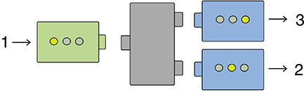
Figure 3. A uniform antidiscrimination setup requires that the obtained measurement outcome is not the sent input put some other index, obtained with uniform probability. Even if such a setup would exist, the setup may not be broadcastable. This is the case e.g. for three inputs and a qubit system as an information carrier.
Download figure:
Standard image High-resolution imageBy using factorization maps we get an easy proof for the fact that the smallest amount of noise that one needs to add in order to make the scenario broadcastable is either 0 or 1. Thus adding white noise to non-broadcastable measurements does not make them broadcastable. This was already observed in slightly different forms in [9, 11, 12].
Proposition 2. Let  and
and  be subsets of measurements and define
  and
and  to be the noisy versions of
  and
and  :
:


where ![$s, t \in (0,1]$](https://content.cld.iop.org/journals/1751-8121/56/13/135301/revision4/aacbc5bieqn164.gif) are fixed noise parameters and
are fixed noise parameters and  denotes the set of coin-toss measurements, i.e. POVMs such that every element is proportional to the identity operator
  . A channel
  passes a broadcasting test
  if and only if it passes a broadcasting test
  .
.
Proof. For any s ≠ 0, the equivalence classes determined by  and
and  are the same. This means that the respective factorization maps are the same, hence the claim follows from proposition 1.
We emphasize that proposition 2 refers to the situation where noisy measurements are measured and the measurement outcome distributions are compared to the expected distributions. In contrast, the optimal quantum cloning device [13, 14] can be seen as performing universal broadcasting at the cost of adding noise to all measurements (see e.g. [15]).
From now on, we will mostly write broadcasting tests in terms of the corresponding factorization maps. This will simplify our calculations as it is easier to consider two maps instead of two subsets of measurements. Moreover, we will use equations (8) and (9) to generalize the idea of broadcasting tests also to broadcasting of channels.
4. Broadcasting of channels
There is a slightly different viewpoint to broadcasting that allows a more flexible starting point. From proposition 1 we conclude that the broadcasting condition demands that Λ copies the test state but is 'invisible' for factorization maps. Instead of factorization maps, we can insert any single-system channels into that condition and this leads to the following definition.
Definition 2. Let  ,
,  , be channels and let
  be a convex set. We say that the triple
  is broadcastable if there exists a channel
  such that for all
  we have


In this case we also say that Φ1 and Φ2 are  -broadcastable.
The conditions (15) and (16) can be again seen as a sort of broadcasting test; if we are acting with Φ1 and Φ2 on the duplicates, then it seems like Λ is a perfect broadcasting device.
Definition 2 resembles the definition of compatibility of channels [16, 17], but has a crucial difference. Namely, we recall that two channels  ,
,  , are compatible if there exists a channel
  such that for all
  , we have


Further, Φ1 and Φ2 are called  -compatible if this condition holds for all
  [18]. By comparing equations (15) and (16) to equations (17) and (18) we see that the latter requires that Λ can reproduce the actions of Φ1 and Φ2, while in the former Λ should duplicate the input state and let Φ1 and Φ2 act on the duplicates. In the following we show that broadcastability is a stronger requirement than compatibility, although for some classes of channels they are equivalent properties.
Proposition 3. Let  ,
,  , be channels and let
  be a convex set.
- (a)If Φ1 and Φ2 are-broadcastable, then Φ1 and Φ2 are -compatible.
- (b)Assume that Φ1 and Φ2 are idempotent channels (i.e. and , ). Then Φ1 and Φ2 are -broadcastable if and only if Φ1 and Φ2 are -compatible.


- (a)
- (b)


![$\Phi_1(\mathrm{tr}_{2}[\Lambda(\rho)]) = \Phi_1(\Phi_1(\rho)) = \Phi_1(\rho)$](https://content.cld.iop.org/journals/1751-8121/56/13/135301/revision4/aacbc5bieqn198.gif)
In the following example we demonstrate that broadcastability is a strictly stronger relation for channels than compatibility. (Invertible channels are not broadcastable but can be compatible).
Example 3 Assume Φ1 and Φ2 are channels that are invertible, but we do not require the inverses to be positive. If Φ1 and Φ2 are broadcastable, we can apply the inverse maps to equations (15) and (16) and get ![$\rho = \mathrm{tr}_{2}[\Lambda(\rho)] = \mathrm{tr}_{1}[\Lambda(\rho)]$](https://content.cld.iop.org/journals/1751-8121/56/13/135301/revision4/aacbc5bieqn199.gif) . It follows that Λ is a universal broadcasting device, which contradicts the no-broadcasting theorem. We conclude that a pair of invertible channels is not broadcastable. However, there are compatible pairs of invertible channels. For instance, a partially dephasing channel
. It follows that Λ is a universal broadcasting device, which contradicts the no-broadcasting theorem. We conclude that a pair of invertible channels is not broadcastable. However, there are compatible pairs of invertible channels. For instance, a partially dephasing channel  is invertible for all parameters
  . Two such channels are compatible for suitably small parameters [19, 20].
Factorization maps are special kind of channels. Hence, in the terminology of definition 2 the result of proposition 1 becomes:
Corollary 1. A broadcasting test  is broadcastable if and only if the triple
  is broadcastable.
As for subsets of measurements, we can assign factorization maps for subsets of channels. For our purposes, it is enough to have the following definition for single channels although an analogous definition can be phrased for subset of channels. For  , we define
  if
if  . Let
. Let  be the set of equivalence classes of
  and let
  be the corresponding factorization map. We introduce a map
  on
on  as
as

for all  . This is again well-defined since by construction Φ is constant on the equivalence classes of
  . We therefore have

and the channel Φ hence factorizes through  . We note that
  is the identity map for injective channels Φ.
We will next show that for broadcasting tests one can restrict to the case of broadcastable factorization channels.
Proposition 4. A triple  is broadcastable if and only if the triple
  is broadcastable.
Proof. The proof is almost the same as proof of proposition 1. Let  be the channel that passes the broadcasting test
  . Let
. Let  . We have

from which it follows that

and so we must have

which shows that Λ passes the broadcasting test  .
.
Let us then assume that Λ passes the broadcasting test  and let
  . We have

which shows that Λ passes the broadcasting test  .
.
One can also obtain the same result as above for broadcasting tests with two subsets of channels, similarly as we did earlier with two subsets of measurements. The results and their proofs would be the same.
Moreover one can also boil down the broadcasting of channels to broadcasting of measurements:
Theorem 1. Let  ,
,  be channels and define


Then  is broadcastable if and only if
  is broadcastable.
Proof. The proof follows from  and
and  . We prove the first equality, the second one follows in the same way. Assume that
  . Then there is a measurement
  such that
  and so
  for
for  . Conversely, assume that
  for some
  . Then
  for some
  and we have
  . It follows that we must have
  .
.
5. Special cases
In this section we are going to look closely at special cases of broadcasting of measurements. We have already seen that all other introduced scenarios can be reduced to this one. We will first show that commutativity of the measurements or some measurements and states is sufficient for broadcastability.
Proposition 5. If  and
and  are mutually commuting, then a broadcasting test
  is broadcastable.
Proof. If  and
and  are mutually commuting, then there is an isomorphism
  such that
  and
and  [21, theorem 1], where
  denotes the direct sum of Hilbert spaces and operators respectively. The result easily follows, since measurements of the form
  and
and  act on separate components and are hence straightforward to broadcast.
Commutativity is not a necessary condition, we will provide counter-examples of broadcastable broadcasting tests of the form  in example 4 and
  in example 5 where the respective measurements do not commute.
Proposition 6. If  and
and  are mutually commuting, then a broadcasting test
  is broadcastable.
Proof. We can again use [21, theorem 1] to show that  is isomorphic to
  and, up to an isomorphism, we have
  and
and  , where now
  and
and  are just to ensure proper normalization of ρ. The result follows immediately, since
  measures only the classical information encoded in the probability distribution pk
.
measures only the classical information encoded in the probability distribution pk
.
5.1. The case when

As the first special case we will assume that  , which is a generalization of the case when
  . If all of the measurements in
  commute, then according to proposition 5 the test is broadcastable. This is the case when all of the measurements in
  can be post-processed from a single projective measurement. To be more specific, let
  be the qutrit Hilbert space,
  , with the orthonormal basis
  , and let
  such that
  . Then
  is broadcastable, the channel that passes the broadcasting test is defined as

To see that Λ passes the broadcasting test, simply observe that

and so measuring  will yield the correct probability. In the following example we will show that commutativity is only sufficient but not necessary condition for broadcastability; the main idea is that if we extend the Hilbert space, then we have some freedom in the choice of
  in equation (27).
(Broadcastable but noncommuting measurements in the
(S,A,A)
scenario).
in equation (27).
(Broadcastable but noncommuting measurements in the
(S,A,A)
scenario).
Example 4 Consider the Hilbert space  ,
,  , with the orthonormal basis
  . Let
. Let  and
and  defined for
  as
as

where  is an arbitrary measurement supported on
 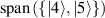 , that is,
  for all
  , and
, and 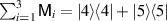 . This implies that
  for all
  and
and  . One can choose
  such that they do not mutually commute, which then implies that also
  do not commute. To see that
  is broadcastable, simply consider channel defined analogically as in equation (27), that is
 ![$\Lambda(\rho) = \sum_{i = 1}^3 \mathrm{tr}\left[\rho \mathsf{A}_i\right] |ii\rangle \! \langle ii|$](https://content.cld.iop.org/journals/1751-8121/56/13/135301/revision4/aacbc5bieqn296.gif) . We again have
. We again have

and the result follows from ![$\mathrm{tr}\left[|i\rangle \! \langle i| \mathsf{A}_j\right] = \delta_{ij}$](https://content.cld.iop.org/journals/1751-8121/56/13/135301/revision4/aacbc5bieqn297.gif) for all
for all  and
and  .
.
Theorem 2. Assume that  . Then
  is broadcastable if and only if there is a single measurement
  such that the norm of every non-zero operator in
  is 1, i.e.
  ,
,  and every measurement in
  can be post-processed from
  , i.e. for every
  and every i we have

where  and
and  .
.
Proof. To see that this is sufficient, we only need to show that  passes the broadcasting test. If
  , then there is unit vector
  such that
  . Since
  , we then must have
  , where λ and µ both index the outcomes of
  . We then construct the channel

We again have ![$\mathrm{tr}_{1}[\Lambda(\rho)] = \mathrm{tr}_{2}[\Lambda(\rho)] = \sum_\lambda \mathrm{tr}\left[\rho \mathsf{G}_\lambda\right] |\lambda\rangle \! \langle\lambda|$](https://content.cld.iop.org/journals/1751-8121/56/13/135301/revision4/aacbc5bieqn318.gif) and the result follows. The proof in the other direction is in the appendix
and the result follows. The proof in the other direction is in the appendix
Corollary 2. Assume that  and that
  . Then
  is broadcastable if and only if for every
  we have that
  and
and  commute for all
  .
.
Proof. Assume that  is broadcastable, the result follows by showing that the measurement
  as described in theorem 2 can be post-processed from a projective measurement. It is then straightforward to show that
  and
and  commute for every
  and for all
  .
.
If  is dichotomic, i.e. it has only two outcomes, then it is commutative, so we need to consider only the case when
  is at least trichotomic, i.e. it has at least three nonzero outcomes. Since then for these three outcomes we must have
  , it follows that we must have at least
  , in which case
  is projective measurement. Thus the only case we need to investigate is when
  and
and  has three nonzero outcomes, since with four nonzero outcomes
  is again projective measurement. So let
  and let
  be a suitable orthonormal basis. Then
 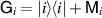 for
for  , which implies that
  for all
  and thus again
  can be post-processed from a single projective measurement.
In the general case when  commutativity is also a sufficient but not necessary criterion for broadcasting. This is demonstrated by the following example, where we use
  to denote the set of operators on the Hilbert space
  .
(Broadcastable but noncommuting measurements in the
(S,A,B)
scenario).
.
(Broadcastable but noncommuting measurements in the
(S,A,B)
scenario).
Example 5 Let  , let
, let  be an orthonormal basis and let
  . Then
  is a four-dimensional Hilbert space, thus it can be seen as tensor product of two qubit Hilbert spaces
  ,
,  , i.e.
 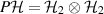 . Moreover let
  be the embedding defined by
  for
for  , that is
 maps operators on
  to operators on
  .
.
Let  be projective measurements on
  given as


where  is an orthonormal basis of
  and
and  .
.
Let  be the partially dephasing channel given as
  . It is known that for
  the channel
  is self-compatible, i.e. there is a channel
  such that
 ![$\Delta_\mu(\rho) = \mathrm{tr}_{1}[\Psi(\rho)] = \mathrm{tr}_{2}[\Psi(\rho)]$](https://content.cld.iop.org/journals/1751-8121/56/13/135301/revision4/aacbc5bieqn374.gif) . We now define measurements
. We now define measurements  ,
,  on
on  such that they do not commute, but are broadcastable. Let


where  is the identity on
  and the terms
  and
and  are supported on
  . In order to construct the channel Λ that passes the broadcasting test
  we will need the auxiliary channel
  defined for
  as
as  and extended by linearity, here we are heavily relying on the identification
 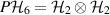 . Then let

where  is the inverse to
 . Λ clearly is completely positive, we only need to prove that it is trace-preserving, but this follows from
 ![$\mathrm{tr}\left[(\Pi(P \rho P)) (P \otimes P)\right] = \mathrm{tr}\left[\rho P\right]$](https://content.cld.iop.org/journals/1751-8121/56/13/135301/revision4/aacbc5bieqn390.gif) and
and ![$\mathrm{tr}\left[(\Pi \circ \Psi \circ \iota^{-1})(P^\perp \rho P^\perp) (P \otimes P)\right] = \mathrm{tr}\left[\rho P^\perp\right]$](https://content.cld.iop.org/journals/1751-8121/56/13/135301/revision4/aacbc5bieqn391.gif) . Finally, to show that Λ passes the broadcasting test
. Finally, to show that Λ passes the broadcasting test  , we have
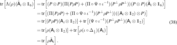
The proof for  is similar.
5.2. The case when is info-complete

It is sufficient that  is informationally-complete. In this case we obtain the following result:
Theorem 3. Assume that  is informationally-complete. If
  is broadcastable, then for every
  there is
  such that
  for all
  and
and  commutes with every
  .
.
Proof. The proof of is in the appendix
Finally we present a simple example that demonstrates why we sometimes need to use  instead of
  .
.
Example 6. Consider the qubit system and assume that  is the set of density matrices diagonal in the computational basis and
  where
where  is the projective measurement corresponding to the eigenvectors of σx
. Clearly there are operators in
is the projective measurement corresponding to the eigenvectors of σx
. Clearly there are operators in  and
and  that do not commute. But note that
 ![$\mathrm{tr}\left[\rho \mathsf{A}_i\right] = \frac{1}{2}$](https://content.cld.iop.org/journals/1751-8121/56/13/135301/revision4/aacbc5bieqn411.gif) for all
for all  and so for
  we have
  and
and ![$[\rho, \tilde{\mathsf{A}}_i] = 0$](https://content.cld.iop.org/journals/1751-8121/56/13/135301/revision4/aacbc5bieqn415.gif) for all
for all  .
.
6. Conclusions
The no-broadcasting theorem is among the most important limitations in quantum information processing. It has, however, very strong assumptions as it uses all states and all measurements in its usual formulation. In the current work we generalized the setting of accurate but limited broadcasting and introduce the concept of a broadcasting test. This enables to pose the question of the exact conditions when broadcasting is possible. Earlier studies have already revealed that commutativity, either between states or measurements, makes broadcasting possible and that is not surprising as the scenario is then effectively classical, but, as we have shown, commutativity is not necessary for broadcasting in general.
We have characterized the conditions for broadcastability in certain important special classes of broadcasting tests. While we did not cover the most general scenario, even the special cases that we have investigated turned out to provide nontrivial and unexpected results. We have also investigated generalizations of broadcasting to channels and we have shown that such generalizations can be mapped back to the case considering only states and measurements.
Future investigations into broadcasting can be done along several lines: one can, of course, attempt to solve the most general scenario, but this will likely be a hard task. Another option would be, in the spirit of [8], to generalize our results to more general systems, such as the ones described by operational probabilistic theories [22] or general probabilistic theories [23, 24]. Yet another line of research would be to consider approximate broadcasting, that is allowed to return the correct result only with some probability, and generalize our result in this direction.
Acknowledgments
This research has been supported by Academy of Finland mobility cooperation funding (Grant No. 434228) and DAAD Joint Research Cooperation Scheme (Project No. 57570110). A J acknowledges support from the Grant VEGA 1/0142/20 and the Slovak Research and Development Agency Grant APVV-20-0069. M P acknowledges support from the Deutsche Forschungsgemeinschaft (DFG, German Research Foundation, Project Numbers 447948357 and 440958198), the Sino-German Center for Research Promotion (Project M-0294), the ERC (Consolidator Grant 683107/TempoQ), the German Ministry of Education and Research (Project QuKuK, BMBF Grant No. 16KIS1618K), and the Alexander von Humboldt Foundation.
Data availability statement
No new data were created or analyzed in this study.
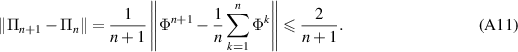
Appendix A: Proof of theorem 2
We denote by  the set of operators on the Hilbert space
  and by
  the set of positive semidefinite operators. We will assume that all of the Hilbert spaces are finite-dimensional.
Definition A.1. Let  be a channel. The adjoint channel (also called the Heisenberg picture)
  is given for
  and
and  as
as

It is straightforward to show that  is a linear and completely positive map and that
  is unital, i.e.
  . The following lemma will play a key role in our calculations. The first one is heavily inspired by [8, lemma 1].
Lemma A.1. Let  be a positive unital map and let

be the set of positive fixed points of Φ. There is a positive map

such that for all  , we have
  and Π is idempotent, i.e.
  . Moreover Π is unital and:
- (a)if Φ is completely positive, then Π is completely positive,
- (b)if Φ is trace preserving, then Π is trace preserving.

then the main idea of the proof is that  . In order to make the limit meaningful we will show that the sequence
  contains a convergent subsequence.
First of all observe that  since Φ is unital. Define

and so for every  we have
  , or, equivalently, for any
  there is
  ,
,  such that
  . Note that
  follows from positivity of Φ and
  follows from
  and again from positivity of Φ. We thus get

Since for every  we have
  and for every Hermitian
  such that
  we have
  , we can express the superoperator norm of Φ as

and using equation (A6) we get  . We then have

which shows that the sequence  is a subset of the unit ball of superoperators. It follows that there is a convergent subsequence
  , see e.g. [25, theorem 28.2]. Denote

Let us first of all show that Π is positive. Let  , then

Since  ,
,  is the limit of positive operators. But then
  since the positive cone
  is closed.
In order to show that  , which is equivalent to
  for
for  , we will need to show that
  converges to the same limit as
  . First note that
Now we have

where we can use equation (A11) and that  converges to Π to show that
  . We now have
and so  for all
  .
.
To show that Π is idempotent we only need to show  for all
  , then
  follows from
  . We have

Since Φ is unital, we have that  and so Π is unital as well.
Finally if Φ is completely positive, then also  is completely positive, which implies that
  is completely positive and so Π is a limit of completely positive maps. It then follows that also Π is completely positive.
If Φ is trace preserving, then

and so Π is also trace preserving.
Theorem 2. Assume that  . Then
  is broadcastable if and only if there is a single measurement
  such that the norm of every non-zero operator in
  is 1, i.e.
  ,
,  and every measurement in
  can be post-processed from
  , i.e. for every
  and every i we have

where  and
and  .
.
Proof. Let Λ be the channel that passes the broadcasting test, then we have  . We can now, without the loss of generality, assume that
  , for example by replacing Λ with
  , which also passes the same broadcasting test whenever Λ does. Here
  is the defined as
  . We then have that
 ![$\mathrm{tr}_{1}[\Lambda(\rho)] = \mathrm{tr}_{2}[\Lambda(\rho)]$](https://content.cld.iop.org/journals/1751-8121/56/13/135301/revision4/aacbc5bieqn488.gif) , thus we define a channel
, thus we define a channel  as
as ![$\Phi(\rho) = \mathrm{tr}_{1}[\Lambda(\rho)]$](https://content.cld.iop.org/journals/1751-8121/56/13/135301/revision4/aacbc5bieqn490.gif) .
.
Since Φ is trace preserving, we have that  is unital and thus, according to lemma A.1, there is a projection
  , where
  , note that we have
  as a consequence of equations (2) and (3), so
  . We will now treat
  as a vector space and
  as a proper cone in
  . We then have the dual vector space
  which contains the dual cone
  . We can now treat
  as a positive linear map and define
  as the trivial embedding of
  into
into  , so that we have that
  is the identity map on
  . The adjoint positive linear maps are
  and
and  and we again have
  . Here
  can be understood as the cone generated by states of some suitable operational theory [23, 24] and
  as the dual cone generated by the effect algebra.
Let us now construct the map  as
as

and we will show that  is a perfect broadcasting map on
  , which then the no-broadcasting theorem [8] implies that
  is a classical cone, i.e. that any base of
  must be a simplex. So let
  and
and  , then we have

where  denotes the pairing between
  and
and  ;
;  follows in the same way. Since
  is generated by a simplex, it follows that there is basis of
  such that every
  is a positive linear combination of gλ
, i.e.
is a positive linear combination of gλ
, i.e.  ,
,  ,
,  , and there are
 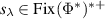 such that
 ![$\mathrm{tr}\left[\Pi^*(s_\lambda)\right] = 1$](https://content.cld.iop.org/journals/1751-8121/56/13/135301/revision4/aacbc5bieqn530.gif) and
and  . Then let
  , then we have that
  since
since ![$\langle s_\lambda, g_\lambda \rangle = \mathrm{tr}\left[\Pi^*(s_\lambda) \mathsf{G}_\lambda\right] = 1$](https://content.cld.iop.org/journals/1751-8121/56/13/135301/revision4/aacbc5bieqn534.gif) where
where  . Moreover for any
  , since
  , we have
 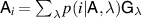 ,
,  follows from the linear independence of
  .
.
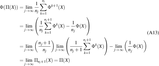
Appendix B: Proof of theorem 3
Let  be a set of states and
  be two sets of POVMs. The triple
  is broadcastable if there exists a channel
  such that equations (2) and (3) hold for all
  ,
,  ,
,  . In other words, there exist two compatible channels
 ![$\Phi_1 = \mathrm{tr}_{2}[\Lambda(\rho)]$](https://content.cld.iop.org/journals/1751-8121/56/13/135301/revision4/aacbc5bieqn548.gif) ,
, ![$\Phi_2 = \mathrm{tr}_{1}[\Lambda(\rho)]$](https://content.cld.iop.org/journals/1751-8121/56/13/135301/revision4/aacbc5bieqn549.gif) such that
such that


for all  ,
,  ,
,  . Assume that
  is information complete, so that the second equality becomes

Since  is a convex set, there is some element
  such that its support contains the supports of all other states in
  . Let
. Let  be the projection onto the support of σ. Note that since
  , we have
 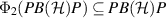 . Let us replace the channels Φ1 and Φ2 with their restrictions to
  , then Φ2 is a channel
  compatible with the channel
  and
and  , so that
  contains a full rank state. According to lemma A.1, there is a unital completely positive idempotent map whose range is the set of fixed points
  . Let Π2 denote the adjoint of this map, then it is easily seen that Π2 is an idempotent channel such that
  . Since compatibility is preserved by post-processing,
  is compatible with Φ1. We may therefore assume that Φ2 is an idempotent channel with a full rank fixed state.
Let us recall some well-known facts, for the convenience of the reader. Let  be an idempotent channel which has a full rank fixed state σ. First, note that the adjoint map
  is an idempotent unital completely-positive map whose range is a subalgebra of
  . Indeed, the range of
  is clearly a self-adjoint linear subspace containing
  , it is therefore enough to prove that
  for all
  . By the Schwarz inequality for unital completely-positive maps [26, proposition 3.3], we have

and since  , we have
 ![$\mathrm{tr}\left[\sigma(\Pi^*(X^*X) - X^*X)\right] = 0$](https://content.cld.iop.org/journals/1751-8121/56/13/135301/revision4/aacbc5bieqn576.gif) , so that
, so that  . Moreover
  is a conditional expectation, which means that it has the conditional expectation property

for  . This can be seen from the fact that
  is multiplicative on its range and [26, theorem 3.18].
The next result extends the well-known equivalence of commutativity and compatibility for projective measurements.
Proposition B.1. Let  be an idempotent channel whose adjoint
  is a conditional expectation and let
  be any channel. Then Φ is compatible with Π if and only if
  and
and  have commuting ranges.
Proof. Let  be the joint channel for Φ and Π, so that the adjoint map satisfies

Since the range of  is a subalgebra in
  , it is generated by projections it contains. It is therefore enough to show that any projection
  commutes with all elements of the form
  ,
,  . We may also restrict to effects,
  , since these generate
  . In this case
  is an effect as well and using the joint channel, it is easily seen that it is compatible with Q. Since Q is a projection, this shows that Q must commute with
  .
.
For the converse, assume that  and
and  have commuting ranges, then the map

is unital and completely positive (e.g. [27, proposition VI.4.23]), and its adjoint is a joint channel for Φ and Π.
Theorem 3. Assume that  is informationally-complete. If
  is broadcastable, then for every
  there is
  such that
  for all
  and
and  commutes with every
  .
.
Proof. We see by proposition B.1 and the paragraph above it that we may assume that Φ1 and Φ2 are compatible channels such that the adjoint of  is a conditional expectation, so that the ranges of the adjoints
  and
and  must commute.
Let  and
and  . Then

By the conditional expectation property of  we have for any
  ,
,

so that  commutes with all other elements in the range of
  . For any
  and
and  :
:

so that Z commutes with ρ. For  , it is now enough to put
  , then
  commutes with all
  and we have
