

Abstract
We discover a series of ring and cluster solitons in the (1+2)-dimensional nonlocal nonlinear fractional Schrödinger equation by iteration algorithm, and verify their robustness by introducing random perturbations during propagations. We obtain the relations between the soliton power, the orbital angular momentum, and the rotation period of phase, which are dependent on the Lévy index α. When the radial number p = 0, the soliton shapes slightly vary with the change of Lévy index. However, when p ≥ 1, the solitons exhibit novel structures, the outer ring (hump) of such solitons decrease as the Lévy index decreases. Our results extend the study of vortex and cluster solitons into fractional systems and deepen the understanding of fractional dimensions.
Export citation and abstract BibTeX RIS
1. Introduction
As early as in 1982, Mandelbrot introduced the concept of fractality in quantum physics [1]. Then Laskin employed space-fractional quantum mechanics to describe the physics when the Brownian trajectories in Feynman path integrals were replaced by Lévy flights [2]. In the past few decades, fractional calculus has been extended to various areas of physics and engineering, such as in anomalous transport [3], electrochemistry [4], diffusion-reaction processes [5], and electromagnetics [6]. In optics, it has also been shown that the fractional diffraction effect exhibits some practical significance [7, 8]. Based on the transverse laser dynamics in aspherical optical resonators, Longhi proposed the optical implementation of the fractional Schrödinger equation [7]. Through utilization of the Dirac–Weyl equation, Zhang et al suggested the honeycomb lattice as a possible realization of the fractional Schrödingere equation system [8]. Various optical beams were discussed in the fractional Schrödingere equation system, such as chirped Gaussian [9] and super-Gaussian beam [10]. Further investigations include solitary waves solutions [11, 12] and numerical solving methods [13, 14] for a fractional Schrödinger equation.
In recent years, it has been revealed that some unique interesting characteristics can result from the nonlocal nonlinearity. For example, nonlocality can suppress the collapse of a (1+2)-dimensional soliton [15], overcome the repulsion between out-of-phase bright solitons [16, 17], and support the propagation of multipole and vortex solitons [18], etc. Hence, a series of novel nonlocal solitons have been discovered in nonlocal nonlinear media, including complicated structure solitons [19], ring dark and antidark solitons [20], spatiotemporal soliton clusters [21], gap solitons [22], variable sinh-Gaussian solitons [23], Hermite–Gaussian stationary solutions [24], higher-order solitons [25], vortex solitons [26], elliptic solitons [27], spiraling elliptic solitons [28], Laguerre–Gaussian (LG) solitons [29], Ince–Gaussian solitons [30], etc. The (1+2)-dimensional solitons have much application value. Especially for the vortex soliton, it can exert forces and torques on the microparticles. In fact, the applications of technologies associated with orbital angular momentum (OAM) range from optical tweezers to microscopy. Questions naturally arise: can ring (including vortex) and cluster solitons be formed in (1+2)-dimensional nonlocal nonlinear fractional Schrödinger equation (NNFSE)? What stability and propagation properties do they have? Usually, the propagation (2+1)-D soliton in the media with the second derivatives and cubic nonlinearity cannot be stable, unless by the addition of linear terms with the first-order derivatives [31], spatial lattice or nonlocality, etc. In this paper, we discuss the existence and propagation stability of ring and cluster solitons in the frame of (1+2)-dimensional NNFSE. The effect of Lévy index on these properties is discussed in detail.
2. Theoretical model
The normalized NNFSE modeling the propagations of (1+2)-dimensional optical beam can be expressed by [11, 32–35]
where ψ is the paraxial optical beam, the transverse coordinates x (y) and longitudinal coordinate z, scaled by the input beam width and Rayleigh length, respectively. (−∂2/∂x2 − ∂2/∂y2)α/2 is the fractional Laplacian and it can be defined as (kx2 + ky2)α/2 in the inverse space for numerical simulation [36], with kx and ky being the spatial frequency. α (1 < α ≤ 2) represents the Lévy index. When α = 2, the NNFSE is reduced to the ordinary nonlocal nonlinear Schrödinger equation (NNSE). It is worth stressing that, the NNFSE in this paper is different from the time-fractional [37, 38] and space-dimension fractional Schrödinger equations [39, 40]. The response function R(x, y) is assumed as Gauss-shaped here
where σ is the characteristic length of the material response function. Although, the Gauss-shaped response function is phenomenological and does not exist in any physical system. The generic properties of the nonlocal soliton can be obtained conveniently by exploiting it. In addition, the physical properties of nonlocal soliton do not strongly depend on the concrete shapes of the response functions [15, 18, 24, 33]. Our numerical results show that the stable soliton cannot form in local and weak NNFSE. Hence, we choose σ = 15 in our numerical simulation hereafter.
For the cylindrical coordinate system, the soliton ψnm in the ordinary NNFSE (α = 2) exhibits an LG-shaped profile [29]. Hence, we choose the LG function as the initial input condition to obtain the ring soliton for 1 < α ≤ 2 in section 3,
and the even and odd LG functions in section 4
where r = (x2 + y2)1/2, A0 represents the amplitude, a0 is the fundamental mode beam width and it was set as a0 = 1 here. Lpm[r2/a02] is the Laguerre polynomial, ϕ = arctan(y/x) is the azimuthal angle. m and p are the topological charge (azimuthal number) and radial number, respectively. According to definition of the second-order moment [19, 29], the beam width of the soliton is
For the LG-shaped beam, apm = (2p + m + 1)1/2 [29], and then a01 = 21/2 and a02 = 31/2. In our numerical simulations, we keep the initial apm invariant (which means that the nonlocal degree apm/σ is unchanged), but change beam profiles and amplitudes throughout the iteration procedures, then the profiles (as shown in figures 1, 4 and 10), critical power (figures 7(a) and 12), OAM (figure 7(b)) and rotation period of phase (figure 7(c)) of solitons for different Lévy indexes are obtained by using the iteration algorithm which was suggested in [33], while, the propagation of the iterative soliton (Φ) in NNFSE is simulated by the split-step Fourier method.

Figure 1. Propagations of ring solitons in NNFSE, and the comparisons of input (red lines, z = 0) and output (dashed blue lines, z = 30) soliton profiles. The parameters are chosen as p = 0, m = 1, a01 = 21/2 for (a1), (a2), and p = 0, m = 2, a02 = 31/2 for (b1), (b2). (a1) α = 2, P01 = 82 004, M01 = 80 807, (a2) α = 1.2, P01 = 35 092, M01 = 34 581, (b1) α = 2, P02 = 83 177, M02 = 164 490. (b2) α = 1.2, P02 = 31 000, M02 = 61 139.
Download figure:
Standard image High-resolution imageThe power and OAM of the iterative soliton can be obtained by [19]
3. Ring-shaped solitons
3.1. Case 1: p = 0
First, we focus on the propagation of single ring, i.e. the (0 1)- and (0 2)-order ring solitons in NNFSE. Figures 1(a1) and (b2) display that, by the iteration simulation, the ring solitons all can be obtained for α = 2 and 1.2, respectively. Comparing figures 1(a1) and (a2) (or (b1) and (b2)), we can find that intensity peaks of solitons decrease as the Lévy index decreases, which can be explained as follows. For fixed beam width, the diffraction is weakened for the decreasing α. To cancel out the weaker diffraction, nonlinearity accounting for the self-focusing will be required at low levels.
By using the iterative solution as the input condition, we found that beams can propagate with the invariant profiles for at least 30 Rayleigh distances, as shown in the fourth column of figure 1. The comparisons of normalized solitons profiles in figure 2 show that the soliton shapes have slight differences for α = 2 and 1.2 when p = 0.
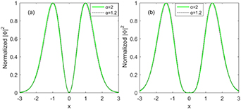
Figure 2. (a) Comparison of normalized (0 1)-order soliton profiles for α = 2 and 1.2. (b) Comparison of normalized (0 2)-order soliton profiles for α = 2 and 1.2. The parameters are the same as in figure 1
Download figure:
Standard image High-resolution imageThe evolutions of solitons phases are displayed in figure 3. Obviously, the phases of both (0 1)- and (0 2)-order ring solitons rotate during the propagation in NNFSE, and the rotation period of phase increases as the Lévy index decreases. The evolutions of power, OAM and rotation period of phase versus the Lévy index will be investigated in detail later.

Figure 3. Phase evolutions of (0 1)- and (0 2)-order ring solitons in NNFSE during propagation. The parameters are the same as in figure 1.
Download figure:
Standard image High-resolution image3.2. Case 2: p ≥ 1
When p ≥ 1, the optical beams have two or more rings, as shown in figure 4. In addition, it is apparent that the normalized intensity of the outer ring decreases as the Lévy index decreases, as seen in figure 5. Similarly to the case of p = 0, the rotation period of phase for vortex solitons at p ≥ 1 increases when the Lévy index decreases, as shown in figure 6.
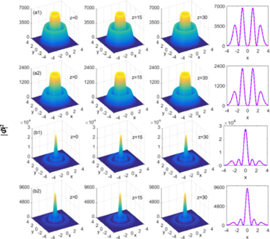
Figure 4. Propagations of ring solitons in the NNFSE, and the comparisons of input (red lines, z = 0) and output (dashed blue lines, z = 30) soliton profiles. The parameters are chosen as p = 1, m = 2, a12 = 51/2 for (a1), (a2), and p = 2, m = 0, a20 = 51/2 for (b1), (b2). (a1) α = 2, P12 = 85 801, M01 = 34 581, (a2) α = 1.2, P12 = 25 290, (b1) α = 2, P20 = 85 901, (b2) α = 1.2, P20 = 25 003.
Download figure:
Standard image High-resolution image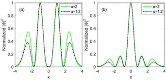
Figure 5. (a) Comparison of normalized (1 2)-order soliton profiles for α = 2 and 1.2. (b) Comparison of normalized (2 0)-order soliton profiles for α = 2 and 1.2. The parameters are the same as in figure 4.
Download figure:
Standard image High-resolution image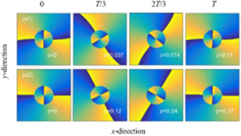
Figure 6. Phase evolutions of (1 2)-order vortex solitons in NNFSE during propagation. The parameters are the same as in figure 4.
Download figure:
Standard image High-resolution imageThe dependences of the powers and the OAMs for solitons on the Lévy index are depicted in figures 7(a) and (b), respectively. As shown in figure 7(a), the powers of different order solitons are almost the same when 1.8 ≤ α ≤ 2. However, when α < 1.8, we can find that the larger the beam width, the smaller the soliton power. It is interesting to note that the power of (1 2)-order soliton is equal to that of the (2 0)-order soliton for any Lévy index. Recalling the fact that the beam widths for these two modes a12 = a20, therefore the modes of (1 2) and (2 0) are degenerate. In fact, all the modes with the same value of 2p + m are degenerate, as found by our numerical results. Comparing figures 7(a) and (b), the OAM is found to be in proportion to the topological change and soliton power, i.e. M ≈ mP. Hence, the OAM of (1 2)-order soliton is smaller than that of a (0 2)-order soliton, even if they have the same topological change when α < 1.8.

Figure 7. (a) Powers and (b) OAMs of the ring solitons versus the Lévy index. (c) Rotation period of phase versus the Lévy index.
Download figure:
Standard image High-resolution imageThe rotation period of phase is shown in figure 7(c), which indicates that the rotation period is increasing as the Lévy index decreases. By comparing figures 7 (a) and (c), we found that the rotation period of phase is in direct proportion to topological change, but inversely proportional to soliton power. After an amount of numerical iterations, we can give an empirical equation, T ≈ 4550 m P−1.
3.3. Stability analysis
To test the robustness of the ring soliton more rigorously, a factor that must be considered is random perturbation, which more or less affects the propagation properties of solitons obtained by numerical iterations. Hence, we introduce a random perturbation by employing the initial condition as A0[G(x, y) + cF(x, y)], where A0 represents the soliton amplitude, G(x, y) stands for the normalized profile of the soliton solution which was obtained by the iteration algorithm, i.e. A0G(x, y) = φ(x, y). F(x, y) is a two-dimensional random matrix with maximum value less than 1, c is a positive coefficient and it is set as c = 0.01 in this paper. Figure 8 demonstrates that vortex solitons can stably propagate under random perturbation. It can also be confirmed by figure 9, which presents the difference of the intensity profiles between the input solitons (red lines) and the output ones (blue lines).
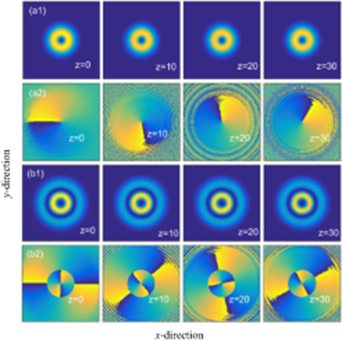
Figure 8. (a1), (b1) Evolutions of soliton intensity propagating with random perturbation. (a2), (b2) Corresponding phase structure to (a1) and (b1), respectively. The parameters of (a1) and (b1) are chosen as in figures 1(a2) and 4(a2).
Download figure:
Standard image High-resolution image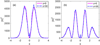
Figure 9. Intensity distributions of the optical solitons at propagation distance z = 0 (red lines) and z = 30 (blue lines). The parameters of (a) and (b) are the same as in figures 8(a1) and (b1), respectively.
Download figure:
Standard image High-resolution image4. Cluster solitons
By using the form of equation (4) as the trial input, we can obtain the cluster solitons by numerical iterations, as shown in figure 10. Similarly to the case of the ring-shaped solitons discussed in section 3, the cluster solitons exhibit almost the same profiles for different Lévy indexes at p = 0, and the outer hump will decrease as the Lévy index decreases when p ≥ 1, which can be shown in figure 11.

Figure 10. Propagations of cluster solitons, and the comparisons of input (red lines, z = 0) and output (dashed blue lines, z = 30) soliton profiles. The parameters are chosen as p = 0, m = 3, a01 = 41/2 for (a1), (a2), and p = 1, m = 2, a02 = 51/2 for (b1), (b2). (a1) α = 2, P01 = 84 194, (a2) α = 1.2, P01 = 28 082, (b1) α = 2, P02 = 85 809, (b2) α = 1.2, P02 = 25 270.
Download figure:
Standard image High-resolution image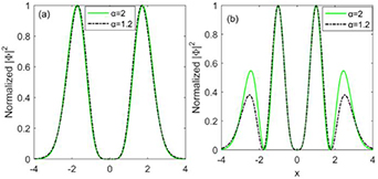
Figure 11. (a) Comparison of normalized (0 3)-order soliton profiles for α = 2 and 1.2. (b) Comparison of normalized (1 2)-order soliton profiles for α = 2 and 1.2. The parameters are all chosen as in figure 10.
Download figure:
Standard image High-resolution imageThe relation between the soliton power and the Lévy index is shown in figure 12, which again indicates the degeneration of the modes with the same value of 2p + m. The cluster solitons are still stable to the random noises during their propagations, which are shown in figures 13 and 14.
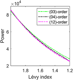
Figure 12. Powers of the cluster solitons versus the Lévy index.
Download figure:
Standard image High-resolution image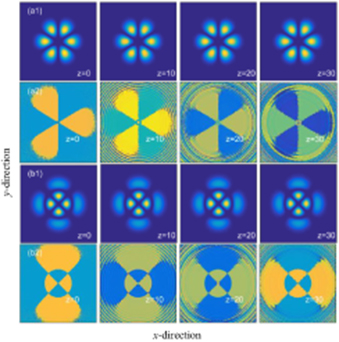
Figure 13. (a1), (b1) Evolutions of solitons propagating with random perturbation. (a2), (b2) Corresponding phase structures to (a1) and (b1), respectively. The parameters of (a1) and (b1) are the same as in figures 10(a2) and (b2).
Download figure:
Standard image High-resolution image
Figure 14. Intensity distributions of the optical solitons at propagation distance z = 0 and z = 30. The parameters of (a) and (b) are the same as in figures 13(a1) and (b1), respectively.
Download figure:
Standard image High-resolution image
5. Summary
The propagations of ring and cluster optical beams in (1+2)-dimensional NNFSE are investigated numerically. Two kinds of solitons are discovered and their properties are found to relatively determine by the Lévy index. Although they exhibit almost the same profiles at p = 0, their normalized outer ring (hump) will decrease as the Lévy index decreases when p ≥ 1. The soliton powers are also found to decrease as the Lévy index decreases. Besides, our numerical results show that all the modes with the same value of 2p + m are degenerate. For the vortex solitons, the phase structures rotate during the propagation, and the rotation velocity increases when the Lévy index increases. All these solitons are robust to the noises.
Since [7, 8, 30] investigated that the equivalent fractional Schrödinger equation can be experimentally realized, and the nonlocality can support various multipole solitons, we deem that our results are helpful to understand the NNFSE, and believe that lots of novel solitons will be found in NNFSEs in the future after this pioneering study.
Acknowledgments
National Natural Science Foundation of China (NSFC) (11847078, 11604199), education department of Jiangxi Province of China (GJJ161043).