THE HELIOTAIL

The heliotail is formed when the solar wind (SW) collides with the local interstellar medium (LISM). From a magnetohydrodynamics (MHD) perspective, the SW–LISM interaction creates a tangential discontinuity that separates the plasmas originating at these two sources. This discontinuity is called the heliopause (HP). Since the SW is superfast magnetosonic at distances of about 10 solar radii, which means that the SW velocity is greater than the fast magnetosonic speed, it decelerates on the inner side of the HP through a so-called heliospheric termination shock (TS). It is convenient to perform numerical simulations in a "heliospheric" coordinate system where the z-axis is aligned with the Sun's rotation axis, the x-axis belongs to the plane defined by the z-axis and the velocity vector ${{\boldsymbol{V}}}_{\infty }$ in the unperturbed LISM and is directed upwind the LISM, and the y-axis completes the right coordinate system. Although the notion of the heliotail is intuitively clear, we will assume that the heliotail starts at distances $x\lt {x}_{0},$ where x₀ is the smallest x on the TS.

It is also convenient to introduce a BV-plane, which is defined by ${{\boldsymbol{V}}}_{\infty }$ and the ISMF vector, ${{\boldsymbol{B}}}_{\infty },$ in the unperturbed LISM. If the SW is spherically symmetric and the heliospheric magnetic field (HMF) is neglected, the BV-plane is the symmetry plane for the SW–LISM interaction. The LISM is only partially ionized, with the number density of neutral H atoms being roughly 3 times greater than the H⁺ ion density. For this reason, neutral atoms play an important role in the SW–LISM interaction (Baranov & Malama 1993; Pauls et al. 1995). By analyzing the Lyα back-scattered emission in the Solar and Heliospheric Observatory (SOHO) solar wind anisotropy (SWAN) experiment, Lallement et al. (2005) discovered a deflection ($\sim 5^\circ$) of the neutral H atom flow in the inner heliosphere from its original direction, ${{\boldsymbol{V}}}_{\infty }.$ These two directions define a so-called hydrogen deflection plane (HDP). Under the above assumption of the SW properties, it is clear that the average deflection occurs parallel to the BV-plane, which was confirmed by Izmodenov et al. (2005) in their kinetic simulations of the H deflection. Kinetic simulations performed by Pogorelov et al. (2008, 2009b) and recently by Katushkina et al. (2015) in the presence of the HMF showed that the deflection parallel to the BV-plane is still dominant, while a smaller deflection perpendicular to this plane also is not negligible. Thus, the property of the BV-plane being nearly parallel to the HDP makes it possible to determine, with some accuracy, the plane where the vector ${{\boldsymbol{B}}}_{\infty }$ belongs. Although the H deflection is also dependent on the angle between ${{\boldsymbol{V}}}_{\infty }$ and ${{\boldsymbol{B}}}_{\infty },$ other measurements are necessary to determine it more conclusively.

One such measurement was provided by the Interstellar Boundary Explorer (IBEX), which identified a bright "ribbon" of the enhanced energetic neutral atom (ENA) flux on the celestial sphere (McComas et al. 2009). Although a number of different explanations were proposed to explain the ribbon, the model of Heerikhuisen et al. (2010) reproduces the ribbon flux within the framework of a self-consistent MHD ion/kinetic (Boltzmann) neutral atoms model. As shown by Pogorelov et al. (2010) and Heerikhuisen & Pogorelov (2011), the position of the ENA ribbon strongly depends on the rotation of the BV-plane about the ${{\boldsymbol{V}}}_{\infty }$ vector, which is usually derived from observations of the He atom flow direction in the inner heliosphere. The most notable measurements of this kind have been performed by Ulysses (Witte 2004) and IBEX (Bzowski et al. 2012; McComas et al. 2015). The kinetic ENA flux simulations of Pogorelov et al. (2009b), Heerikhuisen et al. (2014), and Zirnstein et al. (2015) reproduced the ribbon using the BV-plane nearly parallel to the HDP. The BV-plane remains unchanged even with the modified He velocity vector proposed in Bzowski et al. (2012), although the direction of ${{\boldsymbol{B}}}_{\infty }$ should be changed. However, in this case, the modified (due to the proposed modification of the ${{\boldsymbol{V}}}_{\infty }$ direction by about 5° azimuthally) HDP is at about 30° to the HDP derived from SOHO SWAN observations. This troubling discrepancy has been reconciled by McComas et al. (2015), who showed that the error bars on the IBEX measurements allow the preserving of the ${{\boldsymbol{V}}}_{\infty }$ direction from Ulysses measurements while increasing the LISM temperature from 6250 K to ∼8000 K. In this case, the BV-plane again can be considered to be nearly parallel to the HDP.

Heerikhuisen & Pogorelov (2011), Heerikhuisen et al. (2014), and Zirnstein et al. (2015) have demonstrated that the shape of the ribbon depends on the angle between ${{\boldsymbol{V}}}_{\infty }$ and ${{\boldsymbol{B}}}_{\infty },$ and on the magnitude of ${{\boldsymbol{B}}}_{\infty }.$ This dependence is not as strong as that on the BV-plane angle to the HDP plane. The correlation between the directions toward the ribbon and the lines of sight perpendicular to the ISMF draped around the HP is clearly seen both in MHD-kinetic (Pogorelov et al. 2008, 2009b; Heerikhuisen et al. 2010) and fluid-neutral simulations (Ratkiewicz et al. 2012; Grygorczuk et al. 2014). Funsten et al. (2013) show that the IBEX ribbon is rather circular, although this is not a great circle on the celestial sphere, and the direction of ${{\boldsymbol{B}}}_{\infty }$ is almost toward the ribbon center. In simulations, the deviation is different for different ISMF strengths and directions, but depends very little on particle energy. Additionally, it is clear that the ${\boldsymbol{B}}\cdot {\boldsymbol{R}}=0$ surface, where the ribbon ENAs are born in the model, approaches the plane ${{\boldsymbol{B}}}_{\infty }\cdot {\boldsymbol{R}}=0$, with the increase of ${B}_{\infty },$ i.e., for stronger ISMF, the ribbon approaches the great circle (Pogorelov et al. 2011). Since in reality the ribbon half-angle is about 74° (Funsten et al. 2013), magnetic fields greater than 3 $\mu {\rm{G}}$ should possibly be excluded. Zank et al. (2013) arrive at the same conclusion by analyzing the Lyα absorption in directions to nearby stars.

Voyager 1 crossed the HP in 2012 and started measuring the ISMF strength in the draped region (Burlaga et al. 2013). Although these are one-point-per-time measurements, they also provide restrictions on the direction and strength of ${{\boldsymbol{B}}}_{\infty }.$ For example, the numerical simulations of Pogorelov et al. (2009b) provided ${\boldsymbol{B}}\cdot {\boldsymbol{R}}=0$ directions that were consistent with the IBEX ribbon (McComas et al. 2009; Frisch et al. 2010). The same choice of the LISM properties also reproduced the elevation and azimuthal angles in the ISMF beyond the HP (see Pogorelov et al. 2013a; Borovikov & Pogorelov 2014). On the other hand, the HP instability simulation of Borovikov & Pogorelov (2014), which used the LISM properties from Bzowski et al. (2012), overestimated the elevation angle.

Additionally, restrictions on the LISM properties can be derived (Desiati & Lazarian 2013; Schwadron et al. 2014; Zhang et al. 2014) by fitting the anisotropy of 1–10 TeV cosmic rays observed in air shower observations by the Tibet, Milagro, Super-Kamiokande, IceCube/EAS-Top, and ARGO-YGB teams (see the references in Zhang et al. 2014). According to Zhang et al. (2014), modifications to the unperturbed ISMF produced by the presence of the HP affect TeV cosmic rays in a way that is consistent with observations, but require large computational regions, especially for higher energies. Additionally, Lazarian & Desiati (2010) point out that ion acceleration due to reconnection in the heliotail may affect observed anisotropies.

For the reasons described above, heliotail simulations are very important, especially because there is no way to view the heliotail's structure from outside. On the other hand, jets and collimated outflows are ubiquitous in astrophysics, appearing in environments as different as young stellar objects, accreting and isolated neutron stars, stellar mass black holes, and supermassive black holes at the centers of active galactic nuclei. Despite the very different length scales, velocities, and composition of these various types of jets, they share many basic physical principles. They are typically long, supersonically ejected flows that propagate through and interact with the surrounding medium, exhibiting dynamical behavior on all scales, from the size of the source to the longest scales observed.

The Guitar Nebula is a spectacular example of an Hα bow shock nebula observed by the Hubble Space Telescope and Chandra (Chatterjee & Cordes 2002). The physics of the interaction is very similar to that of the SW–LISM interaction, but there are substantial differences in the stellar wind confinement topology. Mira's astrotail observed by the Galaxy Evolution Explorer (Martin et al. 2007) extends to 800,000 AU. Carbon Star IRC+10216, on the contrary, exhibits a very wide astropause and a short heliotail (Sahai & Chronopoulos 2010). Signatures of the heliotail have been identified in IBEX ENA measurements (McComas et al. 2013). It was also considered in detail theoretically by Yu (1974).

Numerical modeling and subsequent comparison with remote cosmic ray observations and ENA fluxes may be a good way to explore the heliotail. The important questions are: (1) how far downstream should the solution be extended and (2) how should we specify the exit boundary conditions in the far tail? The flow in the tail behind the TS is subfast magnetosonic, while the unperturbed LISM flow may be either subfast or superfast. It is clear that there is a distance from the Sun where the SW and LISM become indistinguishable. Because of charge exchange of the LISM neutral atoms with the hot heliotail ions, the latter will be continuously substituted with cooler ions with properties of the LISM. This means that there is no need to specify physical boundary conditions at the tail exit boundary, where the flow becomes superfast. A simulation to prove that was performed in an axially symmetric, gas dynamics statement without magnetic fields by Izmodenov & Alexashov (2003), who determined that (1) neutral hydrogen atoms qualitatively change the flow pattern of the SW and the LISM in the tail region via charge exchange; in particular, the HP virtually disappears at distances larger than 5000 AU; (2) at distances above 20,000 AU, the SW becomes indistinguishable from the LISM; and (3) the effect of hydrogen atoms makes the SW supersonic at about 4000 AU. In Figure 1 (top panel), we show that this is also true in the presence of the HMF and ISMF. This simulation is made with a kinetic treatment of neutral H atoms using the SW and LISM parameters from Zank et al. (2013). In this and all subsequent figures, the distances are in AU, densities are in cm⁻³, the magnetic field is in μG, and temperatures are in K. The middle panel of Figure 1 shows the HP colored yellow and blue for solutions with ${B}_{\infty }=3\ \mu {\rm{G}}$ and 4 μG, respectively. This simulation was performed with the assumption of a unipolar HMF, similar to Czechowski et al. (2010), Borovikov et al. (2011), and Opher et al. (2015). Note a large-amplitude instability of the HP, with incursions only slightly depending on the choice of ${B}_{\infty }.$ This contrasts with the multi-fluid solution of Opher et al. (2015), which exhibits a two-lobe structure described theoretically by Yu (1974). A possible reason may be the gas-dynamic treatment of interstellar neutral H in the tail, which suppresses charge exchange across the region separating the lobes due to the H-atom bulk flow deflection. Another consequence is the absence of a transition to a superfast magnetosonic flow that is exactly in this region, when H atoms are treated gas-dynamically. One should also be very careful when specifying characteristics-based boundary conditions at the subfast exit (Kulikovskii et al. 2001). It is interesting to look at the HMF line behavior shown in the bottom panel of Figure 1. The line we chose behaves initially as a Parker spiral diverted tailward by the SW flow. At some distance along the tail, however, the regular structure is destroyed due to the breaking of the Parker field structure.

Zoom In Zoom Out Reset image size

To look closer into the details of such behavior, in the next (one plasma—three neutral fluids) simulation, we ignore the ISMF in our solution, with all parameters taken from Opher et al. (2015), but extend it to larger distances, and look at the distribution of the y-component of ${\boldsymbol{B}}$ in the meridional (xz) plane (see Figure 2(a)). This figure also shows the isoline B_y = 0. It is interesting to see that the SW on the right of the z-axis, where $x-{x}_{\odot }\gt 0,$ has a positive B_y and after crossing the TS it is diverted toward the heliotail. The SW flow with $x-{x}_{\odot }\lt 0$ carries ${B}_{y}\lt 0$ below the isoline B_y = 0. This means that the Parker, tornado-like magnetic field is circling around this line. As seen from Figure 2(c), the plasma temperature in the vicinity of the B_y = 0 line decreases from $\sim 1.4\times {10}^{6}$ K immediately beyond the TS to $\sim 8.7\times {10}^{5}$ K at the point where the plasma density starts increasing due to magnetic tension in the Parker spiral. In agreement with Yu (1974), we observe (Figure 2(b)) an increase in plasma density inside the spiral field due to magnetic field tension. It is clearly seen that the B_y = 0 line becomes non-smooth due to the kink instability of a twisted magnetic field (Roberts 1956; Opher et al. 2015) at about 1100 AU from the Sun along the tail, which is consistent with the solution shown in the bottom panel of Figure 1. When the regular Parker field is destroyed, the reason of plasma accumulation inside the spirals disappears, and we observe an increased density level mostly near the highly oscillating line B_y = 0. The distributions of plasma β (the ratio of the thermal pressure to the magnetic pressure $\beta =8\pi p/{B}^{2}$) and $| {\rm{\nabla }}\times {\boldsymbol{B}}|$ shown in panels d and e, respectively, reveal that the flow collimation decreases thermal pressure near the HP, making $\beta \lt 1$ there, while magnetic field gradients inside the spiral field are large. This results in substantial currents in the vicinity of the line B_y = 0. One can see that β is very large (40–10,000) in the vicinity of the line B_y = 0. This is because the poloidal component in the Parker field is lower than the toroidal component. Therefore, β greatly increases in the regions where the toroidal component is small.

Zoom In Zoom Out Reset image size

A vertical cross-section of the heliotail by the plane x = 200 (panel f ) shows a two-lobe structure, in partial agreement with Opher et al. (2015).

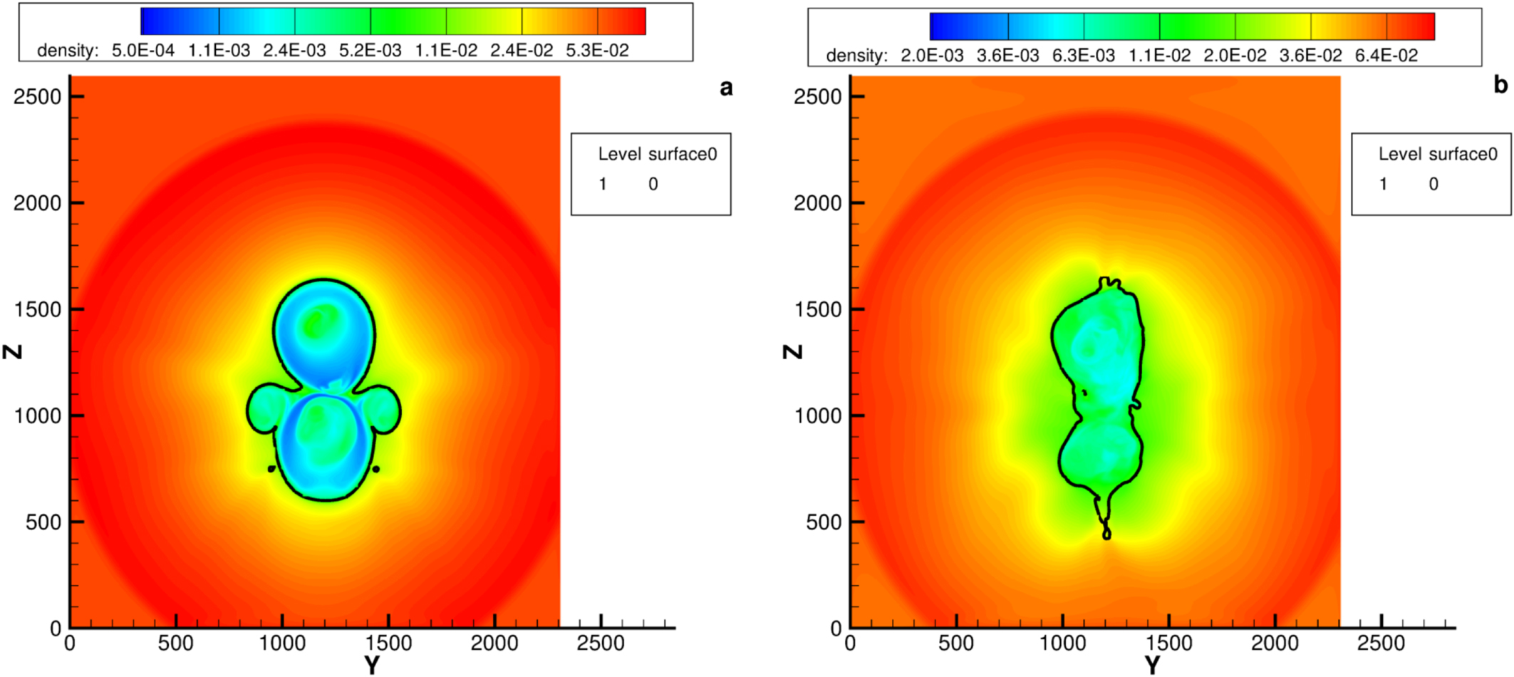
Introducing a unipolar HMF is not necessary to observe the instability of the twisted magnetic field. However, even for a flat current sheet, two-lobe structures disappear if the HMF is a genuine Parker field, characteristic of the situation when the Sun's magnetic and rotation axes coincide (Figure 3).

Zoom In Zoom Out Reset image size

By all means, the assumptions of the unipolar HMF and invariable tilt between the Sun's magnetic and rotation axes are not realistic. It is known that solar cycle effects may explain many Voyager observations: (1) an extended period of sunward flow at V1 (Decker et al. 2012; Pogorelov et al. 2009a, 2012); (2) the distances and timing of the TS crossings by V1 and V2 (Pogorelov et al. 2013b);  and (3) a decrease in the heliocentric distance to the HP (Borovikov & Pogorelov 2014), etc. Zhang et al. (2014) have shown that the orientation of the solar-cycle-affected heliotail in space creates anisotropies in the TeV cosmic ray fluxes. Figure 4 shows the distributions of the plasma density n (a), B_y (b), $| {\boldsymbol{B}}|$ (c), and temperature T (d). The LISM properties are chosen in agreement with McComas et al. (2015) and the IBEX ribbon fitting is performed similarly to Heerikhuisen et al. (2010): ${n}_{\infty }=0.082$ cm⁻³, ${T}_{\infty }=8000$ K, ${V}_{\infty }=26.6\;\mathrm{km}\;{{\rm{s}}}^{-1},$ and ${B}_{\infty }=3$ μG. The unit vectors in the directions of ${{\boldsymbol{V}}}_{\infty }$ and ${{\boldsymbol{B}}}_{\infty }$ are $(-0.996,0,-0.089)$ and $(0.831,-0.353,0.429),$ respectively. Additionally, the neutral H density is ${n}_{{\rm{H}}\infty }=0.172$ cm⁻³. The SW parameters at 1 AU are the following: ${n}_{\mathrm{Es}}=6.9$ cm⁻³, ${n}_{\mathrm{Ef}}=2.4$ cm⁻³, ${V}_{\mathrm{Es}}=450$ $\mathrm{km}\;{{\rm{s}}}^{-1},$ ${V}_{\mathrm{Ef}}=762$ $\mathrm{km}\;{{\rm{s}}}^{-1},$ ${T}_{\mathrm{Es}}=68,000$ K, ${T}_{\mathrm{Ef}}=245,000$ K, and the radial HMF component is 35 μG. Superscripts s and f refer to the slow and fast SW. The solar cycle is introduced by an 11-year periodic function, with the minimum and maximum extents of the slow wind equal to 28° and 90°, respectively. The angle between the Sun's magnetic and rotation axis is also an 11-year periodic function with the minimum and maximum tilts being 8° and 90°, respectively. Additionally, the HMF polarity changes its sign at every solar maximum, which creates the regions of opposite polarities seen in the B_y distribution. This solution also does not exhibit a two-lobe structure and we see only the usual KH instability of the HP surface. It is seen that the heliotail becomes thinner with heliocentric distance in the meridional plane. However, this is not true in 3D. Figure 5 (left panel) shows the HP shape from a viewpoint that demonstrates that the HP flaring actually increases with distance. It is also clear that the HP is compressed due to the draping effect, approximately in the direction perpendicular to the BV-plane. As mentioned earlier, the heliotail position in space and the ISMF are important for the analysis of TeV cosmic ray anisotropy. Since the proton gyroradius of 10 TeV cosmic rays at ${B}_{\infty }=3$ μG is about 500 AU, it is clear that heliotail simulations should be performed in very large computational boxes. Finally, the distance to the HP in this simulation is about 126 AU in the V1 direction and 128 AU in the V2 direction (Figure 5, right panel). This means that according to this model and with a proper distance scaling, V2 may cross the HP in 5 years.

Zoom In Zoom Out Reset image size

Zoom In Zoom Out Reset image size

We described how LISM properties can be constrained by data from IBEX, SOHO, Voyager, and air shower observations. The heliotail extends more than 5000 AU from the Sun and is affected by the solar cycle. The SW flow collimation within the Parker spirals bent into the heliotail goes away once the twisted magnetic field becomes unstable. A two-lobe structure that was described theoretically by Yu (1974) with a number of simplifying assumptions, and obtained numerically by Opher et al. (2015), does not reveal itself even in the case of a unipolar HMF if the H atom transport is described kinetically, in qualitative agreement with Izmodenov & Alexashov (2015). It also disappears if the HMF is bipolar or when the variability in the angle between the Sun's magnetic and rotation axes is taken into account. Numerical simulations presented here are obtained on a Cartesian adaptive grid that ensured a uniform resolution of 0.9 AU everywhere in the tail. There are no visible changes to the flow if the grid is refined twice in all directions. Because of the tremendous disparity of scales such resolution is insufficient for resolving magnetic reconnection in the global simulation. To address the issues raised by Lazarian & Desiati (2010), local, in-the-box simulations will be necessary.

This work was supported by NASA grants NNX14AJ53G, NNX14AF43G, and NNX15AN72G. This work was also partially supported by the IBEX mission as a part of NASA's Explorer program. We acknowledge NSF PRAC award OCI-1144120 and related computer resources from the Blue Waters sustained-petascale computing project. Supercomputer time allocations were also provided on SGI Pleiades by NASA High-End Computing Program award SMD-13-4187 and on Stampede by NSF XSEDE project MCA07S033.