
Abstract
The nonlinear Schrödinger equation and the coupled Burgers equation illustrate the status of quantum particles, shock waves, acoustic transmission and traffic flow. Therefore these equations are physically significant in their own right. In this article, the new auxiliary equation method has been contrivanced in order to rummage exact wave solutions to previously stated nonlinear evolution equations (NLEEs). We have developed ample soliton solutions and have to do with the physical importance of the acquired solutions by setting the specific values of the embodied parameters through portraying figures and deciphered the physical phenomena. It has been established that the executed method is powerful, skilled to examine NLEEs, compatible to computer algebra and provides further general wave solutions. Thus, the investigation of exact solutions to other NLEES through the new auxiliary method is prospective and deserves further research.
Export citation and abstract BibTeX RIS

Original content from this work may be used under the terms of the Creative Commons Attribution 3.0 licence. Any further distribution of this work must maintain attribution to the author(s) and the title of the work, journal citation and DOI.
1. Introduction
Intricate phenomena habitually turn into nonlinear evolution equations (NLEEs). Therefore, the study of NLEEs has sustained to attract much attention in the recent years. Amazingly, the nonlinear phenomena can be investigated by procedures which are interesting and rationally elementary and has a significant impact on both theory and phenomenology. The exact solutions to nonlinear evolution equations are the important tool to comprehend the various physical events which govern the actual world nowadays. Exact solutions plays a significant role in the study of nonlinear physical phenomena in many fields, such as, water wave mechanics, meteorology, electromagnetic theory, plasma physics, solid-state physics, chemical kinematics, optical fiber, nonlinear optics, biochemistry, mathematical chemistry, mathematical physics etc. Therefore, in the past several decades, many scientists and researchers raced to discover good and new methods for solving NLEEs which are important to explain essential nonlinear problems. For example of these methods, the Hirota's bilinear transformation method (Zhou and Ma 2017), the Backlund transform method (Arnous et al 2015), the inverse scattering method (Ablowitz and Musslimani 2016), the first integral method (Tascan and Bekir 2010), the exp-function method (Ma et al 2010), the tanh-function method (Bekir 2009, Abdel et al 2011), the Jacobi elliptic function method (Ma et al 2018), the  -expansion method (Bekir and Guner 2013; Bekir and Cevikel 2009), the extended
  -expansion method (Roshid et al 2014, Alam and Belacem 2015), the improved
  -expansion method (Redi et al 2018), the new generalized
  -expansion method (Alam 2015, Alam and Stepanyants 2016, Alam and Li 2019), the generalized and improved
  -expansion method(Akbar et al 2012a, 2012b). The Weierstrass elliptic function method (Ping and Li 2008), the truncated Painleve expansion method (Radha et al 2007), the functional variable method (Khan and Akbar 2014), the
  -expansion method (Alam and Belacem 2016; Khater 2016, Alam and Tunc 2016, Alam and Alam 2017), the modified simple equation method (Roshid and Roshid 2018), the auxiliary equation method (Kaplan et al 2015, Akbulut et al 2016), the rational exponential function method (Roshid and Alam 2017), the homotopy perturbation method (Javeed et al 2019), the Riccati equation mapping method (Naher et al 2013), the
  -expansion method (Kaplan et al 2016), etc.
To date, much work has been done by many researchers on solution of so many physically significant nonlinear evolution equations. In this article, we introduce and execute a method named the new auxiliary equation method for constructing analytical soliton solutions to the nonlinear Schrödinger equation and the coupled Burgers equation which are important NLEEs to comprehend the phenomena: quantum particles, shock waves, acoustic transmission and traffic flow. Bibi et al (2017) implemented the method and established closed form wave solutions to some NLEEs through this method.
2. The new auxiliary equation method
Suppose, the general nonlinear evolution equation is of the form

Here F is a nonlinear function of u's and u = u(x, y, z, t) is the wave function to be evaluated.
Step 1: We consider the traveling wave variable

The wave variable (2.2) transforms the NLEE (2.1) into an ODE as follows

where prime meaning the ordinary derivative with respect to ξ.
Step 2: As per the new auxiliary equation method, the exact solution of (2.3) supposed to be

where  are constants to be calculated, such that
  and f(ξ) is the solution of the nonlinear equation

Step 3: Balancing the nonlinear terms and the highest order derivatives, we find the positive integer N concerning in equation (2.4).
Step 4: In equation (2.3), we insert equations (2.4) and (2.5) and collecting all the terms having powers of  to zero. As a result of this insertion, yields a system of algebraic equations. This system can be probed to determine the values of ci, k, l, h, w etc.
The solution of equation (2.5) are obtained as follows:
Case 1: When  and
and  ,
,

or

Case 2: When  and
and  ,
,

or

Case 3: When  and
and  ,
,

or

Case 4: When  and
and  ,
,

or

Case 5: When  and r = p,

or

Case 6: When  and r = p,

or

Case 7: When  ,
,

Case 8: When r p < 0, q = 0 and  ,
,

or

Case 9: When q = 0 and  ,
,

Case 10: When p = r = 0,

Case 11: When p = q = K and r = 0,

Case 12: When q = r = K and p = 0,

Case 13: When q = p + r,

Case 14: When  ,
,

Case 15: When p = 0,

Case 16: When  ,
,

Case 17: When r = q = 0,

Case 18: When p = q = 0,

Case 19: When r = p and q = 0,

Case 20: When r = 0,

Substituting the values of the constants ci, p, q and r obtained in step 4 and f(ξ) into (2.4), yield abundant wave solutions to the equation (2.1).
3. Formulation of the soliton solutions
In this section, the nonlinear Schrödinger equation and the coupled Burgers equation containing parameters are studied to found the traveling wave solutions by making use of the new auxiliary equation method.
3.1. The nonlinear Schrödinger equation
Let us consider the NLSE of the form (Biswas and milovic 2010)

where F is a real valued algebraic function and it is important to have the smoothness of the complex function  Considering the complex plane C as a two-dimensional linear space R2, the function
  is k times continuously differentiable so that

In equation (3.1.1), q is dependent variable and x, t are the independent variable, and the subscripts represent the partial derivative of q with respect to that variables. The first term in (3.1.1) represents the time evolution term, while the second term is due to the group velocity dispersion and the third term represents nonlinearity, where a and b be the coefficient of second and third term respectively. Equation (3.1.1) is a nonlinear partial differential equation (PDE) of parabolic type which is not integrable, in general. For simplicity here we use the special case,  , also known as the Kerr law of nonlinearity. In this article, we consider the subsequent NLSE,

The nonlinear Schrödinger equation (NLSE) plays a vital role in various fields of physical, biological and engineering science. It appears in many applied areas, including nonlinear optics (Trikia and Biswasb 2011), plasma physics (Shukla and Eliasson 2010) and protein chemistry (Molkenthin et al 2010). In 1973, Hasegawa and Tappert showed that the NLSE is the appropriate equation to describe nonlinear optical light pulse propagation through optical fibers (Hasegawa and Tappert 1973).
We seek the travelling wave solutions of the NLSE given in equation (3.1.3). In order to search the wave solutions to the NLSE with Kerr law nonlinearity, we introduce the following wave transformation:

Setting the transformation (3.1.4) into (3.1.3), equation (3.1.3) transforms into the following,

Separating real and imaginary parts, equation (3.1.5) yields

and

Therefore, from (3.1.6), we obtain

Therefore, equation (3.1.7) becomes

Balancing the highest order derivative term  with the highest power nonlinear term u3, gives n=1.
According to the new auxiliary equation method, from equation (2.4), the solution of equation (3.1.9) is of the form

where,  is the solution of the nonlinear equation (2.5).
Now, by means of the solution (3.1.10) and (2.5) from equation (3.1.9), we obtain
Setting the coefficients  to zero leads to a set of algebraic equations


Solving the above algebraic equations with the aid of Maple, yields

For the above values of the constants, we attain the subsequent solutions to the NLSE.
Case 1: When  and
and  ,
,
Making use of (3.1.11) and (2.6), (2.7) into equation (3.1.10), we obtain

or

Case 2: When  and
and  ,
,
Putting (3.1.11) and (2.8), (2.9) into equation (3.1.10), we achieve

or

Case 3: When  and
and  ,
,
Applying (3.1.11) and (2.10), (2.11) into equation (3.1.10), we accomplish

or

Case 4: When  and
and  ,
,
Exerting (3.1.11) and (2.12), (2.13) into equation (3.1.10), we attain

or

Case 5: When  and r = p,
Employing (3.1.11) and (2.14), (2.15) from equation (3.1.10), we ascertain

or

Case 6: When  and r = p,
Making use of (3.1.11) and (2.16), (2.17) from equation (3.1.10), we gain

or

Case 7: When  ,
,
By means of (3.1.11) and (2.18) from equation (3.1.10), we find out

Case 8: When rp < 0, q = 0 and  ,
,
Inserting (3.1.11) and (2.19), (2.20) into equation (3.1.10), we derive

or

Case 9: When q = 0 and  ,
,
Setting (3.1.11) and (2.21) into equation (3.1.10), we secure

When p = r = 0, and p = q = K, r = 0, inserting the values of the constants lead to constant solutions and hence has not been documented here, since constant solutions have no physical significance.
Case 10: When q = r = K and p = 0,
Using (3.1.11) and (2.24) into equation (3.1.10), we obtain

Case 11: When q = p + r,
Applying (3.1.11) and (2.25) into equation (3.1.10), we attain

Case 12: When  ,
,
Inserting (3.1.11) and (2.26) into equation (3.1.10), we secure

Case 13: When p = 0,
By means of (3.1.11) and (2.27) from equation (3.1.10), we ascertain

Case 14: When  ,
,
Making use of (3.1.11) and (2.28) from equation (3.1.10), we gain

When r = q = 0, and r = 0 embedding the values of the constants lead to constant solutions and hence has not been written here, since constant solutions have no physical significance.
Case 15: When p = q = 0,
Using (3.1.11) and (2.30) into equation (3.1.10), we carry through

Case 16: When r = p and q = 0,
Using (3.1.11) and (2.31) from equation (3.1.10), we obtain

It is observe that, by means of the new auxiliary equation method, we obtain abundant closed form traveling wave solutions of the NLSE, which might be useful to analyse various complex phenomena in physical sciences, nonlinear optics, fluid dynamics, mathematical biology, plasma physics and other areas.
3.2. The coupled Burgers equation
In this section, we will examine the homogeneous form of the coupled BE equation. We consider the following system of equations (Jawad et al 2010):


where α and β are arbitrary constants.
In fluid mechanics, Burgers equation is one of the crucial model equations (Rezazadeh et al 2019). In addition these equations are used to narrate the structure of shock waves travelling in a viscous fluid (Mittal and Rohila, 2018), traffic flow and acoustic transmission.
In order to study equations (3.2.1) and (3.2.2), we introduce the subsequent travelling wave transformations
 and ξ = x − λ t.
Hence equations (3.2.1) and (3.2.2) take the form


Integrating equations (3.2.3) and (3.2.4) and considering the integration constants to zero, since we are searching for soliton solutions, the equations (3.2.3) and (3.2.4) become


Now balancing the highest order derivative term  with the highest order nonlinear term U2 and UV gives n = 1, m = 1.
Therefore, according to new auxiliary equation method, the solution of equations (3.2.5) and (3.2.6) take the form


where,  is the solution of the nonlinear equation (2.5).
Inserting equations (3.2.7) and (3.2.8) together with equations (3.2.5) and (3.2.6), we achieve

and
Now, setting the coefficients  to zero leads to a set of algebraic equations:


Solving these algebraic equations with the aid of Maple, we achieve


Now by using the above values of the constants, we attempt to establish the wave solutions to the coupled Burgers equation.
Case 1: When  and
and  ,
,
Using (3.2.9), (2.6) and (2.7), from equation (3.2.7), we achieve

or

Using (3.2.9), (2.6) and (2.7) into equation (3.2.8), we accomplish

or

Case 2: When  and
and  ,
,
Putting (3.2.9), (2.8) and (2.9) into equation (3.2.7), we get

or

Putting (3.2.9), (2.8) and (2.9) into equation (3.2.8), we attain

or

Case 3: When  and
and  ,
,
Applying (3.2.9), (2.10) and (2.11), from equation (3.2.7), we ascertain

or

Applying (3.2.9), (2.10) and (2.11), from equation (3.2.8), we find out

or

Case 4: When  and
and  ,
,
Exerting (3.2.9), (2.12) and (2.13) into equation (3.2.7), we derive

or

Exerting (3.2.9), (2.12) and (2.13) into equation (3.2.8), we secure

or

Case 5: When  and r = p,
Employing (3.2.9), (2.14) and (2.15), from equation (3.2.7), we determine

or

Employing (3.2.9), (2.14) and (2.15), from equation (3.2.8), we carry out

or

Case 6: When  and r = p,
Making use of (3.2.9), (2.16) and (2.17), from equation (3.2.7), we carry through

or

Making use of (3.2.9), (2.16) and (2.17), from equation (3.2.8), we carry through

or

Case 7: When  ,
,
By means of (3.2.9) and (2.18), from equation (3.2.7), we obtain

By means of (3.2.9) and (2.18), from equation (3.2.8), we obtain

Case 8: When  and
and  ,
,
Inserting (3.2.9), (2.19) and (2.20), from equation (3.2.7), we accomplish

or

Inserting (3.2.9), (2.19) and (2.20), from equation (3.2.8), we accomplish

or

Case 9: When q = 0 and  ,
,
Setting (3.2.9) and (2.21) into equation (3.2.7), we get

Setting (3.2.9) and (2.21) into equation (3.2.8), we get

Whenever p = r = 0 and p = q = K, r = 0, embedding the values of the constants lead to steady solutions and thus has not been reported here, since consistent solutions have no physical essentialness.
Case 10: When  and p = 0,
Exerting (3.2.9) and (2.24) into equation (3.2.7), we attain

Exerting (3.2.9) and (2.24) into equation (3.2.8), we ascertain

Case 11: When q = p + r,
Employing (3.2.9) and (2.25), from equation (3.2.7), we gain

Employing (3.2.9) and (2.25) into equation (3.2.8), we gain

Case 12: When  ,
,
Making use of (3.2.9) and (2.26), from equation (3.2.7), we find out

Making use of (3.2.9) and (2.26), from equation (3.2.8), we find out

Case 13: When p = 0,
By means of (3.2.9) and (2.27), from equation (3.2.7), we derive

By means of (3.2.9) and (2.27), from equation (3.2.8), we derive

Case 14: When  ,
,
Inserting (3.2.9) and (2.28) into equation (3.2.7), we secure

Inserting (3.2.9) and (2.28) into equation (3.2.8), we secure

Whenever r = q = 0 and r = 0 implanting the values of the constants lead to consistent arrangements and subsequently has not been composed here, since steady arrangements have no physical essentialness.
Case 15: When p = q = 0,
Putting (3.2.9) and (2.30) into equation (3.2.7), we determine

Putting (3.2.9) and (2.30) into equation (3.2.8), we determine

Case 16: When r = p and q = 0,
Using (3.2.9) and (2.31) into equation (3.2.7), we carry out

Using (3.2.9) and (2.31) into equation (3.2.8), we carry out

It is perceive that by means of the new auxiliary equation method, we have achieved abundant closed form traveling wave solutions to the coupled Burgers equation, which might be helpful to explore simplest nonlinear model of turbulence, the motion of the isolated waves and many fields such as hydrodynamics, plasma physics, nonlinear optic etc.
4. Results and discussion
In this section, we have interpreted the obtained solutions to the nonlinear Schrödinger equation and the coupled Burgers equation through depicting some three dimensional figures of the attained solutions with the aid of symbolic computation software Mathematica. In this segment, we have represented the some graphs (Figure 1–7) of the obtained solutions to the nonlinear Schrödinger equation to visualize the shape of all of the obtained solutions. From the solutions, it is observed that, we attain trigonometric solutions (3.1.12), (3.1.13), (3.1.16), (3.1.17), (3.1.20), (3.1.21), (3.1.32) and (3.1.34) and hyperbolic solutions (3.1.14), (3.1.15), (3.1.18), (3.1.19), (3.1.22), (3.1.23), (3.1.25) and (3.1.26). We achieve rational solution (3.1.24) and (3.1.33), and exponential solution (3.1.27)–(3.1.31).
The solutions (3.1.12), (3.1.13), (3.1.20), (3.1.21) and (3.1.34) represent the nature of singular periodic wave solution.
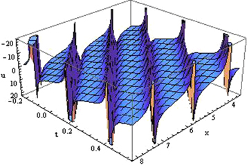
Figure 1. Plot of the singular periodic shape solution (3.1.12) for the value of 
Download figure:
Standard image High-resolution imageThe solutions (3.1.14), (3.1.16), (3.1.18), (3.1.22) and (3.1.25) represent the nature of kink wave solution.
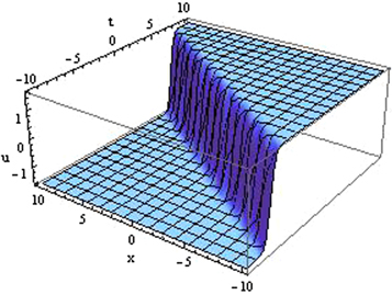
Figure 2. Plot of the kink shape solution (3.1.14) for the value of 
Download figure:
Standard image High-resolution imageThe solutions (3.1.15)–(3.1.17), (3.1.19), (3.1.23), (3.1.24), (3.1.26), (3.1.27), (3.1.28)–(3.1.31) and represent the nature of singular kink wave solution.
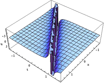
Figure 3. Plot of the singular kink wave shape solution (3.1.15) for the value of 
Download figure:
Standard image High-resolution imageIn this section, we analyze the solution of the coupled Burgers equation attained in this study. It is observed that the secured solutions (3.2.10)–(3.2.13), (3.2.18)–(3.2.21), (3.2.26)–(3.2.29), (3.2.50), (3.2.51), (3.2.54) and (3.2.55) are presented in trigonometric function and are presented in hyperbolic function of the solutions: (3.2.14)–(3.2.17), (3.2.22)–(3.2.25), (3.2.30)–(3.2.33) and (3.2.36)–(3.2.39). Again the solutions (3.2.34), (3.2.35), (3.2.52) and (3.2.53) are obtained in rational function. And the solutions (3.2.40), (3.2.41) and (3.2.42)–(3.2.49) are obtained in the form of exponential function.
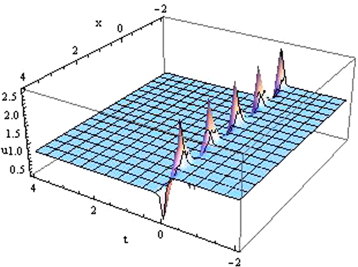
Figure 4. Plot of the absolute value of the spike shape solution (3.2.10) for the value of p = 3, q = 1, r = 2, α = 5, β = 2.
Download figure:
Standard image High-resolution imageThe absolute value of the solutions (3.2.10)–(3.2.13), (3.2.18)–(3.2.21) and (3.2.26)–(3.2.29) represent the nature of spike shape wave solution.
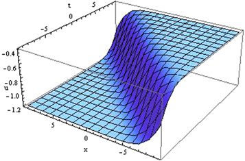
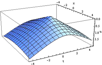
Figure 5. Plot of the kink shape soliton solution (3.2.14) for the value of p = 1, q = 3, r = 2, α = 3, β = 2.
Download figure:
Standard image High-resolution imageThe solutions (3.2.14), (3.2.16), (3.2.22), (3.2.24), (3.2.38), (3.2.30), (3.2.32), (3.2.36) and (3.2.55) represent the nature of kink wave solution.
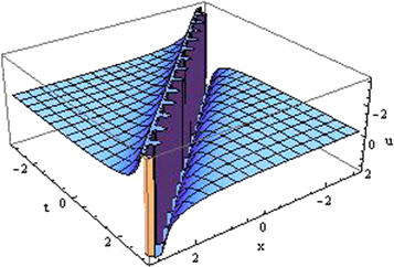
Figure 6. Plot of the singular kink wave soliton solution (3.2.15) for the value of p = 1, q = 3, r = 2, α = 3, β = 2.
Download figure:
Standard image High-resolution imageThe solutions (3.2.15), (3.2.17), (3.2.23), (3.2.25), (3.2.31), (3.2.33), (3.2.37), (3.2.39)–(3.2.41), (3.2.46)–(3.2.53) represent the nature of singular kink wave solution.
Figure 7. Plot of the compacton soliton solution (3.2.50) for the value of p = 1, q = 1, r = 1, α = 3, β = 2.
Download figure:
Standard image High-resolution image
And the solutions (3.2.50) and (3.2.51) represent the nature of compacton wave solution.
5. Conclusion
In this article, the analytical soliton solutions to the nonlinear Schrödinger equation and the coupled Burgers equation have been successfully obtained by executing the new auxiliary equation method with less computational effort. We have established the solitary wave solutions as well as periodic wave solutions, singular periodic wave solutions, kink shape soliton, singular kink shape soliton, bell shape soliton, singular bell shape soliton and compacton wave solution of nonlinear evolution equations by choosing arbitrary values of the free parameters. The solutions are found by trigonometric, hyperbolic, rational, exponential function by using this method. The obtained solutions are quite practical, well suited and useful. This study demonstrated that the new auxiliary equation method is an influential and efficient technique in searching exact solutions for wide class of problems and can also be applied to other kind of complicated nonlinear problems. We might conclude that the suggested method can be prolonged to solve the nonlinear problems that arise in the theory of solitons and other areas.
Acknowledgments
The authors would like acknowledge the anonymous referees for their valuable comments and suggestions on our manuscript. This work is supported by the USM Research University Grant 1001/PMATHS/ 8011016 and the authors acknowledge this support.