
Abstract
An ameliorated salp swarm algorithm (ASSA) is proposed to enhance the exploration and exploitation stages of the basic salp swarm algorithm using the concept of opposition based learning and position updation. These concepts not only resolve the issue of slow convergence but also reduces the computation time and circumvent strucking in local minima. Based on ASSA, an improved adaptive variational mode decomposition (VMD) method has been proposed to identify the impeller fault in the centrifugal pump. The optimal combinations of VMD parameters: mode number and quadratic penalty factor, are selected adaptively to decompose the vibration signal. On decomposition, the sensitive mode is identified for the extraction of fault features. The basis of identification of sensitive mode is a maximum value of weighted kurtosis. The ranking of fault features is done by Pearson correlation coefficient (PCC). The ranked features train the extreme learning machine (ELM) model and further, the model is tested for fitness evaluation. The overall training accuracy of the ELM model is found to be 100% with 0.0012 seconds of training time. The testing accuracy was found to be 97.5%. Results obtained at twenty-three classical benchmark functions and the Wilcoxon test validate the efficiency and superiority of the proposed ASSA algorithm in the diagnosis of centrifugal pump impeller faults.
Export citation and abstract BibTeX RIS
1. Introduction
A centrifugal pump is an essential unit in the process industry that generates pressure head by rotating its impeller. The rotating impeller is mounted on a shaft supported by bearings. The involute casing of the rotating impeller forces the flowing water to impart velocity [1]. Corrosion by reactive chemicals, erosion by solid slurry particles, the existence of any metallurgical flaws, cavitation, poor lubrication, and mechanical defects are some of the causes of centrifugal pump failure [2]. The two major components that are prone to failure are the bearing and the impeller. Both vibration and acoustic signals help in monitoring the condition of the centrifugal pump [3]. Acoustic signals are generally affected by environmental noise. Therefore, the vibration-based fault identification method is preferred in the proposed work.
Researchers have been working extensively in the fields of sophisticated signal processing and machine learning [4–9] to identify problems in centrifugal pumps. Azizi et al [10] applied empirical mode decomposition (EMD) to determine the severity of cavitation in centrifugal pumps and further classified them using the generalized regression neural network (GRNN). Pan et al [11] proposed sympletic geometric mode decomposition techniques to decompose the raw signal for removing the noise and further reconstructing the components based on corresponding eigenvalues obtained through similarity transformation. Pan et al [12] extracted the sensitive features that describe the defect conditions of the rotating machinery through data-driven adaptive Fourier spectrum segment making use of modified empirical wavelet transform. Yan et al [13] improved the Kolmogorov complexity and incorporated it with singular spectrum decomposition (SSD) along with the idea of multi-channel processing to diagnose the wind turbine. Kumar and Kumar [14] proposed the GA-SVM model to classify different defects using features obtained from the raw signal and the scale marginal integration (SMI) signal. Even though the genetic algorithm showed its effectiveness while predicting the faults but it stuck in local minima and have a slow convergence speed which needs to be addressed. Kumar et al [15] diagnosed the faulty bearing using a symmetric cross-entropy of neutrosophic sets for an axial pump. Ali et al [16] extracted features based on EMD energy entropy and further trained the artificial neural network (ANN) classification model to identify bearing defects. Jena and Panigarhi [17] utilized Wavelet packet transform (WPT) for locating defect bursts in gear and bearing automatically. For defect diagnosis of a reciprocating compressor, Zhang et al [18] employed an optimised convolution deep belief network. Alves et al [19] used a deep convolution neural network to diagnose an oval defect in a journal bearing.
Dragomiretskiy introduced variational mode decomposition (VMD) as a new signal decomposition approach [20]. It decomposes the signal into intrinsic modes whose centre frequency is computed online, so that extracted mode synchronizes accordingly. Dragomiretskiy proved that VMD is better than EMD for tone detection and tone separation. Kumar et al [1] proposed the VMD method for fault identification of a centrifugal pump using a cross-entropy measurement index. Ye et al [21] diagnosed the rolling bearing by VMD and reconstructed the modes based on feature energy ratio Further, the authors extracted the multidimensional feature vectors using multiscale permutation entropy for different defect conditions and classified them by particle swarm optimization-based support vector machine (PSO-SVM). Zhang et al [22] used VMD to fragment signals to discover a bearing defect in a multistage centrifugal pump. The VMD parameters viz, mode number, and quadratic penalty factor are generally determined based on experience. This greatly affects the performance of VMD and sometimes leads to inaccurate decomposition results [23]. The optimal combination of parameters is the primary requirement for VMD based decomposition. Shi and Yang [24] optimized both parameters of VMD independently in the diagnosis of the wind turbine. Yan et al [25] used a genetic algorithm to optimise VMD parameters, with the envelope spectrum entropy value serving as the fitness function.
Other optimization techniques are also used to optimize VMD parameters. Swarm intelligence (SI) techniques are one of them, which are inspired by nature and imitates the swarming behaviour of various organisms such as ants, a flock of birds, a school of fish, etc [26]. Gravitational search algorithm (GSA), particle swarm optimization (PSO), sine cosine algorithm (SCA), hybrid genetic algorithm and particle swarm optimization (HGPSO), grasshopper optimization algorithm (GOA), whale optimization algorithm (WOA), grey wolf optimizer (GWO) and ant colony optimization (ACO) are some examples of SI techniques, used to solve the different optimization problems [27–29]. Jin et al [30] proposed the pricing formulas for uncertain fractional first-hitting model on the basis of reliability index and Asian barrier. Deng et al [31] enhanced the differential evolution (DE) optimization algorithm by incorporating the mutation strategy. The improved DE on CEC'08 at a different number of populations is applied to show its effectiveness. Guo et al [32] optimized the reward function of the deep Q network (DQN) to plan the path of the coastal ships. Jin et al [33] formulated the hitting time model on the basis of an uncertain fractional-order differential equation with the Caputo type reliability index and European barrier pricing formula.
An opposition and position updation based ameliorated salp swarm algorithm (ASSA) is proposed in this paper to develop adaptive VMD for vibration signal so that the defect in the centrifugal pump could be identified. By doubling the initial population size and position updation, the proposed algorithm not only enhances convergence speed but also decreases the computation time and cost. It also minimises chances of strucking in local minima while in search of the optimal combination of VMD decomposition parameters. The weighted kurtosis is utilised as a fitness function to find the best optimal parametric settings for VMD and is further used to select the sensitive mode from which defect features are extracted. The Pearson correlation coefficient (PCC) technique is used to rank extracted features which is an indicator of the impact of each feature on the signal. The PCC also eliminates the redundancy of data. The selected features are used to train the ELM and determine the training and testing accuracy. The rest of the paper is organised as follows.
Section 2 addresses the theoretical concepts. Section 3 provides the methodology and novelty in the proposed work. The detailing of experimentation has been discussed in section 4 briefs about test rig, data acquisition and feature extraction. Section 5 discusses the results obtained from the classical benchmark function and Wilcoxon test for the proposed algorithm, and the same is compared with other art of optimization techniques. The comparison of the proposed optimization algorithm has been done with the basic salp swarm algorithm in terms of convergence speed. In the end, section 6 summarizes the conclusion of the study. The definitions of the benchmark functions and the comparison of the proposed optimization algorithm ASSA with other art of optimizations are discussed in the
2. Theoretical basis
2.1. Variational mode decomposition (VMD)
VMD decomposes the raw vibration signal into different modes  having the sparsity with the original signal. The modes thus obtained must be centred on a central frequency
  In the frequency domain, the sparsity of the mode
  is selected as the bandwidth [20, 34]. The following procedure is adopted to obtain the bandwidth of the mode: (1) Hilbert transform extracts the mode
  in order to draw frequency spectrum, (2) The obtained frequency spectrum is shifted to 'baseband' which is close to its respective central frequency, (3) In the end,
  norm computes the frequency bandwidth. The raw signal is decomposed in the following manner which is shown in equation (1) [20]:


where, the input signal is represented by  the set of modes are indicated by
  central frequency is represented by
  whereas Dirac distribution
  represents convolution. To make the optimization problem given in the equation (1) unconstraint, the Penalty factor
  (data fidelity constraint) and Lagrangian multiplier λ is used. The obtained unconstraint problem is shown in equation (2).

Equation (2) is solved by the alternate direction method of multipliers (ADMM) that gives the sequence of sub-optimization to find the saddle point. The obtained solutions of sub-optimization of ADMM directly optimizes the problem mentioned in equation (2) in the Fourier domain [20]. The detailed procedure of the algorithm is given in [20]. The modes  and central frequency
  updates their values according to the ADMM optimization problem. The equation (2) updates the variational mode function (VMF) with respect to
  and after updating the VMF, the sub optimal problem is given in equation (3).

The Fourier transform with tuned centre frequency helps in finding the optimum solution for equation (3). The modes  updates their values through equation ( 4).

The Wiener filter is used to filter the signal prior to  for current residual signal. The spectrum of each mode (
 ) is obtained by Hermitian symmetric completion. The inverse Fourier transform of the real part of the filtered signal gives modes (uk
) in the time domain. Equation (2) is optimized in such a way that the centre frequency does not originate in the reconstruction fidelity. The desired problem is defined in [20]:
) is obtained by Hermitian symmetric completion. The inverse Fourier transform of the real part of the filtered signal gives modes (uk
) in the time domain. Equation (2) is optimized in such a way that the centre frequency does not originate in the reconstruction fidelity. The desired problem is defined in [20]:

Equation (5) is solved by the optimization to obtain the centre frequency which is shown in equation (6)

The centre frequency wk in equation (6) is updated as per their corresponding mode at the centre gravity of the power spectrum.
The above equations suggested that four parameters viz, mode number (K), quadratic penalty factor (α), tolerance (τ), and convergence criterion (ε) are required in the procedure of VMD and need to be specified in advance. τ and ε usually adopt their default values, taken in original VMD as these parameters have little effect on decomposition results. But mode number K need not be specified in advance without having prior knowledge of the signal to be analyzed. As nothing can be said about the appropriateness of K and thus, it cannot ensure the accuracy and efficiency of decomposition results. Quadratic penalty factor α suppresses the noise interference in the signal and also controls the frequency bandwidth, thus should be chosen accordingly. The optimal selection of the combination of parameters is the key to VMD and is the motivation of the research.
2.2. Extreme learning machine (ELM)
ELM is a method used for both regression and classification purposes [35]. The single-layer feed-forward network (SLFN) is the foundation block of ELM as shown in figure 1. In ELM there are basically three layers viz, input, hidden, and output layers. For  arbitrary samples
  SLFN having
  hidden nodes and activation function
  is mathematically modelled as given in equation (7) [23, 35]:

Here,  and
and  are learning parameters of hidden nodes, out of which
  connects the input weight vector of input nodes to ith hidden node and
  denotes the threshold of the ith hidden node.
  and
and  represents output weight and test point whereas activation function
  gives output for ith hidden node. The equation can be written in matrix form as shown in equation (8).

where,

and

As per ELM theories, the values of  and
and  are randomly assigned for all hidden nodes instead of being tuned. The solution of the above equation is estimated by using equation (11).

where,  is inverse for the output matrix
  Moore-Penrose's generalized inverse is utilized for this purpose. The steps involved in the ELM algorithm is summarised below:

Figure 1. Extreme learning, machine (ELM) structure.
Download figure:
Standard image High-resolution imageStep 1: Assigning learning parameters i.e.  and
and  of the hidden nodes randomly,
Step 2: Hidden layer output matrix  is to be calculated.
Step 3: Inverse of the hidden layer output matrix is calculated using Moore-Penrose generalized inverse.
3. Proposed scheme
An adaptive VMD procedure is proposed by optimizing its parameters, i.e., mode number K, and the quadratic penalty factor  for vibration signal analysis. To make VMD adaptive, the optimal combination of parameters is selected by a particular search rule, which is based on two main criteria. One criterion is the construction of the measurement index, and another is the search method, i.e., the optimization technique. An ameliorated salp swarm algorithm is developed as a new search method utilizing opposition-based learning and position updating concept which searches the best optimal parameters adaptively for VMD. The sensitive mode among the various decomposition modes of VMD for fault identification is selected based on weighted kurtosis which is introduced as a novel measurement index that is formed by hybridising the kurtosis and correlation coefficient. This coefficient takes density distribution into account, which is generally neglected by kurtosis. Once the sensitive mode is selected, features are extracted and an extreme learning machine is applied to automatically identify the defect in the pump.
3.1. Weighted kurtosis index
The measurement index is the key element for making VMD adaptive, which determines the efficacy of the decomposition results. Literature suggested that kurtosis and correlation coefficients are two important indices for fault diagnosis of rotating machines through vibration signals [36]. Kurtosis index is mainly dependent on the density distribution of impacts generated by fault. Hence, impacts having a large amplitude but with dispersing density distribution is neglected, if maximum kurtosis index is used as a candidate solution or fitness function to optimize parameters of VMD. The correlation coefficient quickly determines the similarity between two signals, but it is prone to the noises present in the signal of faulty components [36]. Their hybrid index i.e., weighted kurtosis index is built to assist as a fitness function to find optimal VMD parameters [37]. The weighted kurtosis index ( ) is given in the following equation (12).

where  represents the kurtosis index for input signal
  and expressed as

Here, the length of the signal is given by  Considering
 ![$E\left[.\right]$](https://content.cld.iop.org/journals/2631-8695/3/3/035041/revision2/erxac23b5ieqn40.gif) a mathematical expectation, the correlation
a mathematical expectation, the correlation  between
  and
and  is expressed as

3.2. Ameliorated salp swarm algorithm for optimizing VMD parameters
Mirjalili et al [38] proposed the swarm intelligence (SI) based salp swarm algorithm (SSA) optimization technique. It imitates the swarm behaviour of salps or a chain of salps for food foraging in the deep ocean. In SSA, the initial random population is divided into two sections viz, leaders, and followers to construct the mathematical model of salp swarm [38]. The leader leads and guides the salp chain, whereas followers follow the leaders through the salp chain.
The basic idea of the salp swarm algorithm (SSA) and an ameliorated salp swarm algorithm (ASSA) proposed in this communication has been explained in the following subsections along with the inspiration behind the modification in SSA. Initialization of population, function evaluation and dividing the swarm are common processes for SSA and ASSA. Opposition-based learning is used to modify SSA and make it faster in terms of convergence. The process of updation of the position of leader and followers is modified through different equations given in respective subsections to design ASSA comprehensively.
3.2.1. Initialization of population
Initially, the population is generated in the search space  in a random manner through uniform distribution as shown in equation (15).

where  indicates the search space,
  represents the populations, and
  is the dimension of search space. The upper bound and lower bound of the search space is denoted by
  and
and  respectively. The population
  is randomly generated in the range of (0,1).
3.2.2. Opposition-based learning
Nature-inspired optimization algorithms start by selecting global optima randomly and then initialize every individual randomly in a given search space. To discover the appropriate solution, each individual updates their position based on its intellect and behaviour. The computation time required by these methods is determined by the initial guesses. However, the computation time can be reduced if these techniques start checking their own opposite solution [39]. One with a better solution, either from randomly generated or its opposite guess, is selected. Starting with a closed guess and verifying it with its fitness function not only lowers computing time but also enhances the convergence speed. This approach can be continuously applied to each solution for the current population, along with initialization. The same concept has been introduced to modify the basic salp swarm algorithm. The initialization of the population in opposition-based learning is done in the following manner as shown in equation (16).

where,  represents the salp population from opposition-based learning.
3.2.3. Computation of fitness function
The fitness of the swarm is evaluated by using equation (17). The best function value,  is obtained mathematically and is written as

where, i = 1, 2, ..., NP
The best salp position is saved corresponding to the best function value, 
3.2.4. Division of the swarm
There is a division of swarms into two groups known as leaders and followers. The percentage of leaders can be varied from 10% to 90% as suggested in [38]. In given research, the leaders and followers are divided in equal numbers i.e., in equal percentages.
3.2.5. Position updation of the leader
Like any other swarm-based optimization technique, the salp position is the candidate solution stored in a two-dimensional matrix called  for
for  -dimensional search problem.
  is the number of design variables. In
  the optimal position represents the best food source called
  The position of leaders is updated as per equation (18).

where  is the position of the leader (first salp),
  is the probability, on the basis of which leader's position is decided and
  is a food source in
  dimension.
  are upper bound and lower bound respectively of
  dimension.
 and
and  are random variables, out of which
  plays a vital role in balancing exploitation and exploration.
  is defined in equation (19) as

Here,  indicates the current iteration, the maximum iteration is represented by
  Random variables
  and
and  are randomly generated between 0 and 1. The probability
  is defined in equation (20) as

where,  represents the fitness of
 indicates the best fitness obtained in all iterations. Equation (20) has been introduced as a modification that helps in updating the position of the leaders.
3.2.6. Position updation of the followers
The follower position is updated according to equation (21), which is based on Newton's Law of Motion.

where 
 indicates the position of ith follower in salp chain of jth dimension. And α is weighting factor defined in following equation (22)

where,

Equations (22), and (23) are incorporated in equation (21) as modifications in the basic salp swarm which updates the follower's position.
The following is the pseudocode for the proposed ASSA Algorithm:
Initialize the salp population NP1  using equation (15).
Apply opposition-based learning on this initial population to get NP2 members.
Calculate objective function on NP1 and NP2 using equation (25).
Select best NP members out of (NP1 + NP2).
Select members,  with best function value and designate as
while

Calculate the objective function of each individual.
Update  by equation (19)
for i = 1: size of salp population
if i <= half of the salp population
generate  and
and  randomly within [0,1]
calculate the value of P using equation (20)
update the position of the leaders using the equation (18)
else if i > half of the salp population
generate the variable var1 using equation (23)
create α using equation (22)
update the position of the follower using equation (21)
end
end
updated salp position
end
amend the salps based on upper and lower bounds of variables.
evaluate the objective function on the updated salp position
update the value xbest and gbest
end
3.3. Pearson correlation coefficient-based feature ranking
In the case of large data, generally, filter type algorithms are used to rank the features. Feature filter is simply the function of correlation or information which returns the relevant index  [40]. This index computes how relevant is the given feature subset
  for task
  which can be a classification or approximation of data
  Relevant index is calculated for each individual feature
  in order to know the ranking order
  Features with lowest rank are generally filtered out. Pearson correlation coefficient (PCC) is one of the methods which determines the rank of features which is based on correlation measurement [40]. PCC is computed by using equation (24):

where  is a feature with value
  and class
  is a class having values
  If
If  is ± 1, then
  and
and  are dependent on each other but if
  is zero, then
  and
and  are uncorrelated. Error function
  is used to compute the probability of how two variables are correlated to each other. Decreasing values of error function
  serve as feature ranking and order the feature list accordingly.
3.4. Fault identification approach
A method to make VMD adaptive is proposed based on ameliorated salp swarm algorithm (ASSA) by using maximum weighted kurtosis as the fitness function as given in equation (25). Here, the original salp swarm algorithm is improved by introducing opposition-based learning in it, thus named ASSA. The proposed optimization algorithm is made to find the minimum value; thus, the required maximization problem is converted into a minimization problem by introducing a negative sign in the fitness function, as shown in equation 25. Ranking of features is also proposed to see how features are relevant to fault diagnosis using PCC. It is further passed through ELM to compute training and testing accuracy.

where, 
 indicates the weighted kurtosis for decomposition modes of VMD.
  are parameters of VMD which are to be optimized. Mode number
  varies in the interval of [2, 7], and the quadratic penalty factor
  takes value in an interval of [1000,10000]. The range for parameters has been decided based on an extensive literature survey [23, 34, 41].
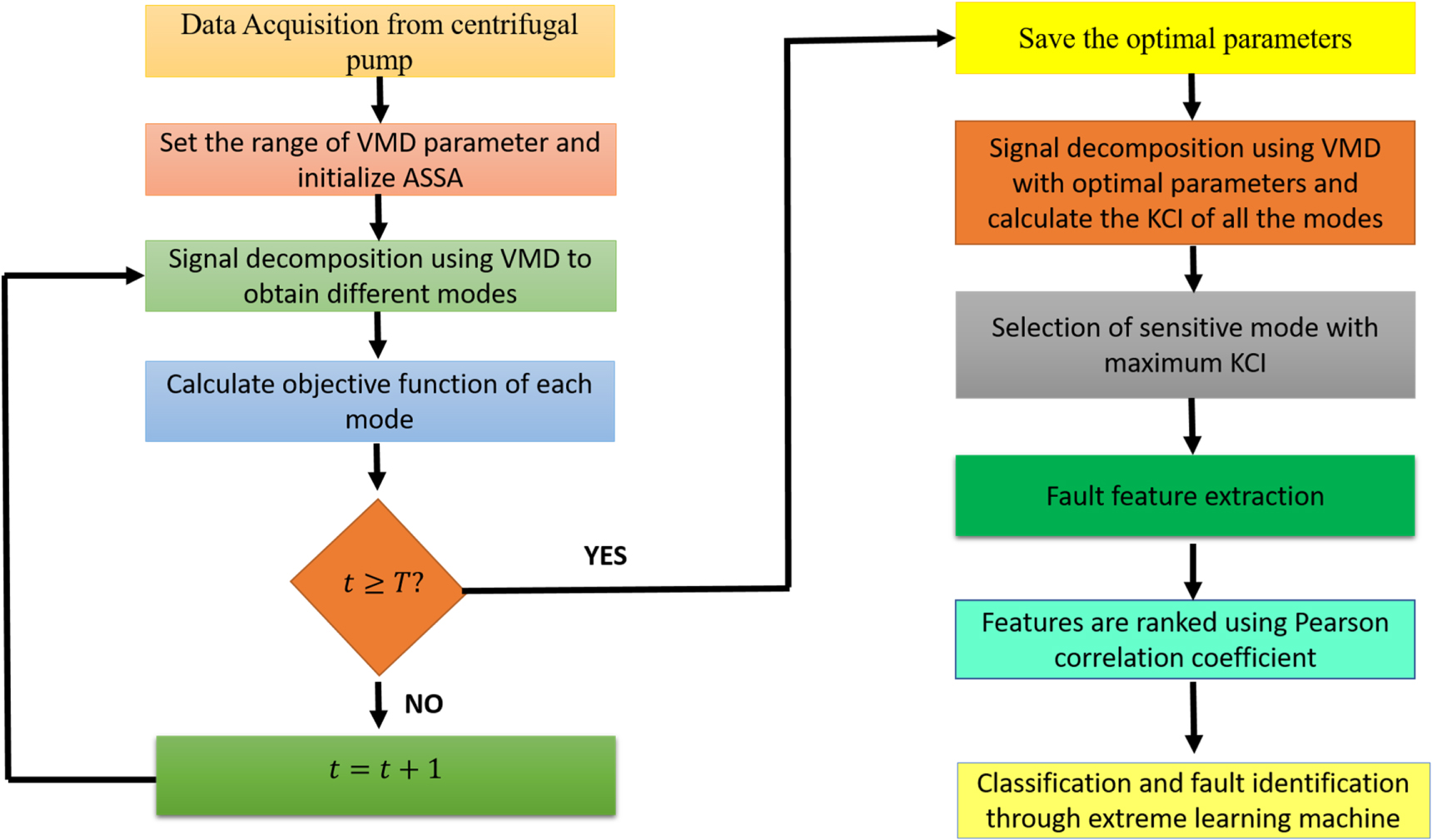
The detailed steps of the proposed work are given below:
- The raw vibration signal is decomposed by VMD with set ranges of parameters that are to be optimized. Store the value of the objective function for each iteration.
- Initialize parameters of ASSA with
 population and number of maximum iterations.
 - Obtain the modes after decomposition of vibration signal using VMD. Then, compute the objective function for each mode.
- If then the required condition is achieved, the iteration will end. Otherwise, put and continue the iteration.
- Save the combination of optimal parameters based on the minimum value of an objective function. And, store the mode corresponding to a maximum weighted kurtosis index, thus known as a sensitive mode.
- Characteristics features are obtained from sensitive mode and arranged in ranked order using PCC. Store the obtained data.
- Further obtained data is feed into ELM to determine the training and testing accuracy of the model.


The whole methodology is shown in the form of flow chart as given in figure 2.

Figure 2. Flowchart for adaptive VMD method for fault identification in the centrifugal pump.
Download figure:
Standard image High-resolution image4. Experimentation
4.1. Test rig
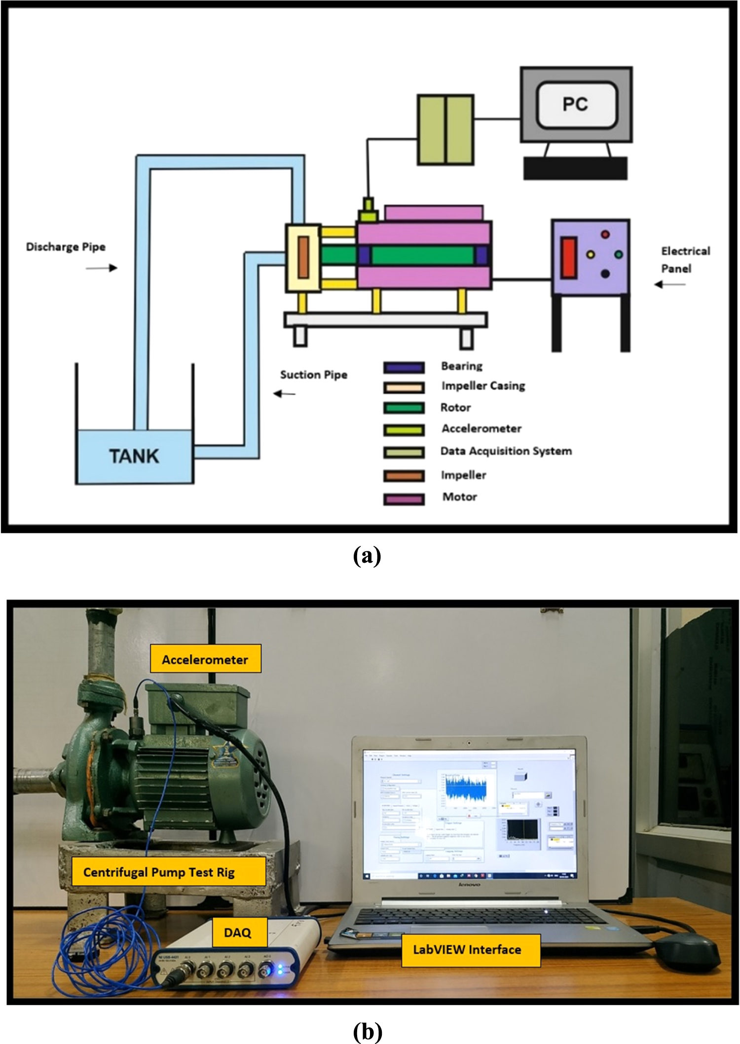
The proposed method was applied to the data set acquired from the test rig of the centrifugal pump. The schematic of the pump test rig and its pictorial view is shown in figures 3(a) and (b), respectively. The pump is operated at 2800 rpm (i.e., 46.67 Hz). The pump's specification is given in table 1. Two bearings are used to support the shaft of the pump. These bearings are named Bearing 1 (closer to impeller; bearing number 6203-ZZ) and Bearing 2 (away from the impeller, bearing number 6202-ZZ). The impeller is attached to the rotor shaft and is encased in a casing. The impeller is made up of revolving vanes that pull water axially through the impeller's eye and impart kinetic energy to the water. This kinetic energy forces the water to flow in a radially outward direction through the casing. This energy gets transferred between water and vanes through impacts which generate the chaotic phenomenon in the water.

Figure 3. (a) Schematic of centrifugal pump (b) a typical photograph of centrifugal pump test rig with an accelerometer placed for data acquisition.
Download figure:
Standard image High-resolution imageTable 1. Specification of centrifugal pump.
| Power supply | 230/240 V |
|---|---|
| Motor power | 0.5 Hp |
| Discharge | 1.61 litre s−1 |
| Impeller type | Closed |
| Impeller diameter | 118 mm |
| Impeller vanes | 3 |
4.2. Data acquisition
The vibration signals are acquired by a uniaxial accelerometer having a sensitivity of 100 mV g−1. The accelerometer is mounted near the impeller casing as shown in figure 3(b). The vibration signal is acquired using a 24-bit, four-channel DAQ of National Instruments make, with a sampling frequency of 70 kHz. To investigate the signal, 0.1 seconds of data with 7000 data points are taken. The study is carried out under various impeller conditions, as illustrated in figure 4. The adaptive VMD technique is used to process the raw signal acquired from the centrifugal test rig. The two parameters of VMD, i.e., mode number (K) and quadratic penalty factor (α), are optimized using ameliorated salp swarm algorithm. The other parameters of VMD are taken, as suggested in [20]. The suggested algorithm ASSA obtains the optimal combination of VMD parameters. With these optimal combinations of parameters, the most prominent mode is selected based on maximum weighted kurtosis. This prominent mode is processed for further analysis.

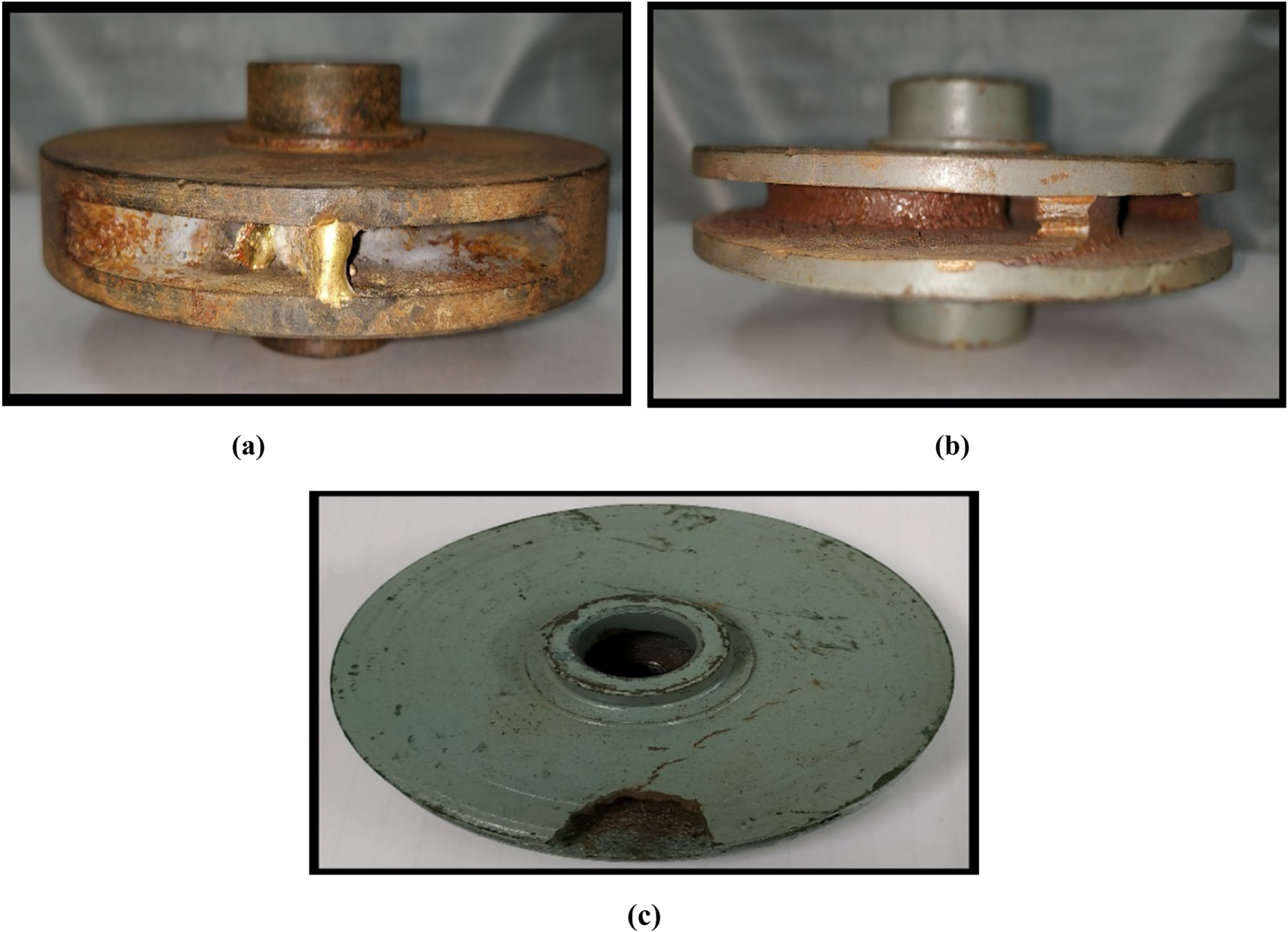
Figure 4. Different operating conditions (a) Clogging (b) Blade cut (c) Wheel cut.
Download figure:
Standard image High-resolution imageInitially, the data is acquired for the pump operating at 2800 rpm (i.e., 46.67 Hz operating frequency) with normal (no defect) impeller in place. The pump has a constant operating speed for all types of impeller conditions under study. The raw signal in the time domain for defect-free impeller condition is shown in figure 5(a). This raw signal is converted into a frequency domain and represented in figure 5(b). The characteristic frequency of 47 Hz is also shown in this figure which is equivalent to the pump operating frequency. Since the pump is operating at constant rpm in all health conditions that's why FFT corresponding to operating frequency will remain the same for every condition. The raw signal is decomposed into different modes by adaptive VMD based on ASSA. From ASSA, the mode number, K and quadratic penalty factor,  comes out to 3 and 1000 respectively. The different modes are shown in figure 5(c). For each mode, the weighted kurtosis is calculated. The third mode has the highest weighted kurtosis value, 12.73, and has been chosen for feature extraction. Twenty signals are collected for examination, with each signal subjected to no-defect, clogged, blade cut, and wheel cut impeller conditions.

Figure 5. (a) Raw signal with non-defective impeller (b) FFT for non-defective impeller (c) Different modes obtained by applying adaptive VMD to the raw signal.
Download figure:
Standard image High-resolution imageSimilarly, under clogged impeller conditions, the data is collected and divided into distinct modes using adaptive VMD with 3 mode number (K) and 4000 quadratic penalty factors, which is optimised by ASSA. In this case, the three modes have weighted kurtosis values of 1.99, 1.95, and 3.08. The third mode has the highest weighted kurtosis value and is thus chosen for further processing. The time-domain signal, frequency domain signal and decomposed modes are shown in figures 6(a)–(c), respectively.

Figure 6. (a) The raw signal under clogged impeller condition (b) FFT under clogged impeller condition (c) Different modes obtained by applying adaptive VMD under the clogged impeller condition.
Download figure:
Standard image High-resolution imageThe raw signal for blade cut impeller condition is shown in figure 7(a). The corresponding frequency domain signal is shown in figure 7(b). The computed optimized value of parameters K and  are 3 and 1000, respectively, for this signal. The raw signal is split into three modes at these parameters, as illustrated in figure 7(c). Weighted kurtosis values for the first, second, and third modes are 1.62, 1.60, and 8.62, respectively. The third mode was chosen for further examination because it has the highest value of weighted kurtosis.

Figure 7. (a) The raw signal under blade cut impeller condition (b) FFT under blade cut impeller condition (c) Three modes obtained by applying adaptive VMD under blade-cut impeller condition.
Download figure:
Standard image High-resolution imageThe time-domain signal for the wheel-cut impeller condition is shown in figure 8(a) and the corresponding frequency signal is shown in figure 8(b). Following the process described in the previous scenarios, the optimal settings for mode number and penalty factor are 3 and 2000, respectively. The three obtained modes are depicted in figure 8(c). The weighted kurtosis for the first, second, and third modes, respectively, is 1.54, 3.87, and 11.63. As a dominant mode, the mode with 11.63 as weighted kurtosis is chosen.

Figure 8. (a) The raw signal under wheel-cut impeller condition (b) FFT under wheel-cut impeller condition (c) Different modes obtained by applying adaptive VMD under wheel-cut impeller condition.
Download figure:
Standard image High-resolution image4.3. Feature extraction
The adaptive VMD technique based on ASSA yields a total of 80 significant modes of vibration signals (20 each for healthy (no-defective), clogged, blade cut, and wheel cut impeller conditions) employing weighted kurtosis as a measurement index. Following that, eleven features are retrieved from prominent modes decomposed through adaptive VMD. Table 2 provides a list of features and their definitions. The features extracted are normalized in the range of [0 1] using the following mathematical expression:

Table 2. Extracted features with their definition.
| S. no. | Features | Definitions |
|---|---|---|
| 1. | Standard Deviation ( ) ) |

|
| 2. | Peak ( ) ) |

|
| 3. | Skewness ( ) ) |

|
| 4. | Kurtosis ( ) ) |

|
| 5. | Root Mean Square ( ) ) |

|
| 6. | Peak Factor (PF) |

|
| 7. | Square Root Amplitude ( ) ) |

|
| 8. | Shape Factor (SF) |

|
| 9. | Impulse Factor (IF) |

|
| 10. | Wavelet Packet Decomposition (WPD) Energy |

|
| 11. | Permutation entropy |

|
Here,  represents data;
  represents the number of data points;
  is the average value of
 represents the decomposition coefficient for
  sequence and
  is the level of
  decomposition.
5. Result and discussion
5.1. Comparison of the ASSA with other art of optimization
The efficacy of the proposed optimization algorithm (ASSA) is tested on twenty-three classification functions. These functions are widely used in literature and defined in table A1 at annexure. The proposed optimization algorithm ASSA is compared with other art of optimizations i.e., SSA, GWO, GOA, SCA and HGPSO in terms of mean, standard deviation, best, worst and median. The comparison is given in table A2. Based on the minimum value of standard deviation, ASSA proved its superiority in nineteen benchmark functions that are Sphere, Schwefel 2.22, Schwefel 1.2, Schwefel 2.21, Rosenbrock, Quartic, Rastrigin, Griewank, Penalized, Penalized 2, Foxholes, Kowalik, Six-hump camel back, Branin, Goldstein-price, Hartman 3, Shekel 5, shekel 7 and shekel 10. For Schwefel and Ackley, the techniques SCA and GWO show better results. HGPSO shows the best results for Step and Hartman 6 benchmark functions. Results obtained showed the overall effectiveness of ASSA in comparison to other optimization techniques.
Over 20 separate runs, the algorithms on classical functions were compared using mean, standard deviation, best, worst, and median. This, however, does not compare the particular run. This suggests that excellence may be acquired through accident. As a result, it is critical to compare the outcomes of each run and determine the significance of the results. To determine the significance level of each run, the Wilcoxon rank-sum statistical test was performed at a 5% significance level and the corresponding P-values for each benchmark are computed and tabulated in table 3. If the P-values are less than 0.05, it is strong evidence against the null hypothesis. This also implies that the best method produced better final objective function values that did not happen by coincidence. For the statistical analysis, the best algorithm in each test function is chosen and separately compared with other algorithms. The best algorithm in the given study is chosen based on the lowest standard deviation value. If there are many algorithms with the same standard deviation, the one with the lowest mean value is the best. Because the best algorithm cannot be compared to itself, N/A, which stands for Not Applicable, has been written for the best algorithm in each function.
Table 3. P-values calculated for the Wilcoxon rank sum-test (significance level 0.05) corresponding to the results in table A2.
| Function | ASSA | SSA | GWO | GOA | SCA | HGPSO |
|---|---|---|---|---|---|---|
| F1 | N/A | 6.7860 × 10−08 | 6.7956 × 10−09 | 6.7956 × 10−08 | 6.7956 × 10−08 | 6.7956 × 10−08 |
| F2 | 6.7956 × 10−08 | 6.7956 × 10−08 | 6.7956 × 10−08 | 6.7956 × 10−08 | 6.7956 × 10−08 | N/A |
| F3 | N/A | 6.7860 × 10−08 | 6.7656 × 10−09 | 6.7956 × 10−08 | 6.7956 × 10−08 | 6.7956 × 10−08 |
| F4 | N/A | 6.7478 × 10−08 | 6.7956 × 10−08 | 6.7956 × 10−08 | 6.7956 × 10−08 | 6.7956 × 10−08 |
| F5 | N/A | 0.0411 | 6.7956 × 10−08 | 0.0962 | 0.0337 | 1.7936 × 10−04 |
| F6 | N/A | 0.0720 | 6.7956 × 10−08 | 0.0810 | 6.9756 × 10−08 | 6.776 × 10−08 |
| F7 | N/A | 6.7956 × 10−08 | 6.7956 × 10−08 | 6.7956 × 10−08 | 6.9756 × 10−08 | 0.1075 |
| F8 | 6.7765 × 10−08 | 1.2346 × 10−07 | 6.7956 × 10−08 | 6.5970 × 10−08 | N/A | 6.5997 × 10−08 |
| F9 | N/A | 7.9043 × 10−09 | 7.4517 × 10−09 | 8.0065 × 10−09 | 0.0096 | 7.8321 × 10−09 |
| F10 | N/A | 7.9334 × 10−09 | 7.6187 × 10−09 | 8.0065 × 10−09 | 1.6310 × 10−07 | 3.3187 × 10−09 |
| F11 | N/A | 8.0065 × 10−09 | 0.0402 | 8.0065 × 10−09 | 6.6826 × 10−05 | 9.4038 × 10−06 |
| F12 | N/A | 0.7972 | 6.7956 × 10−08 | 6.7956 × 10−08 | 6.7956 × 10−08 | 4.9511 × 10−08 |
| F13 | N/A | 0.0026 | 6.7956 × 10−08 | 1.2493 × 10−05 | 6.7860 × 10−08 | 7.7336 × 10−05 |
| F14 | N/A | N/A | 6.4846 × 10−05 | N/A | 3.5055 × 10−07 | N/A |
| F15 | 5.4753 × 10−05 | 8.0065 × 10−09 | 0.0055 | 1.5253 × 10−06 | 1.0352 × 10−06 | N/A |
| F16 | N/A | N/A | 1.1129 × 10−07 | N/A | 7.9919 × 10−09 | 7.9919 × 10−09 |
| F17 | N/A | N/A | 8.0065 × 10−09 | N/A | 8.0065 × 10−09 | N/A |
| F18 | N/A | N/A | 7.9919 × 10−09 | N/A | 7.991 × 10−09 | N/A |
| F19 | 8.0065 × 10−09 | N/A | 8.0065 × 10−09 | 8.0065 × 10−09 | 8.0065 × 10−09 | 8.0065 × 10−09 |
| F20 | 2.8636 × 10−08 | 2.7747 × 10−08 | 3.0480 × 10−04 | 2.8836 × 10−08 | 6.7956 × 10−08 | N/A |
| F21 | N/A | 0.0057 | 0.2616 | 0.3637 | 6.7956 × 10−08 | 0.3637 |
| F22 | N/A | 2.7769 × 10−07 | 0.0859 | 4.4162 × 10−05 | 1.2346 × 10−07 | 4.4162 × 10−05 |
| F23 | N/A | 8.3337 × 10−04 | 0.9246 | 6.0054 × 10−04 | 1.2330e-07 | 8.3337e-04 |
As it can be seen from the table, ASSA obtained the best results for 18 functions i.e., F1, F3-F14, F16-F18, and F21-F23. For other functions such as F8 and F19, SCA and SSA respectively show better results. HGPSO is selected as the best algorithm for F2, F15 and F20. As per results in tables 4 and 5, ASSA performs better than other compared algorithms, which demonstrates that the superiority of this algorithms is statistically significant. According to the No-free lunch theorem (NFL) theorem [42], it can solve the problem that cannot be solved efficiently by other algorithms.
Table 4. Weight of each feature obtained after applying PCC.
| S. No. | Features | Weight of features |
|---|---|---|
| 1. | Standard Deviation ( ) ) | 0.2743 |
| 2. | Peak ( ) ) | 0.0552 |
| 3. | Skewness ( ) ) | 0.0789 |
| 4. | Kurtosis ( ) ) | 0.1435 |
| 5. | Root Mean Square ( ) ) | 0.5223 |
| 6. | Peak Factor (PF) | 0.0552 |
| 7. | Square Root Amplitude ( ) ) | 0.0711 |
| 8. | Shape Factor (SF) | 0.1619 |
| 9. | Impulse Factor (IF) | 0.0259 |
| 10. | Wavelet Packet Decomposition (WPD) Energy | 0.0915 |
| 11. | Permutation entropy | 0.0850 |
Table 5. Comparison of performance of different classification techniques with the proposed method along with training time.
| S.no. | Classification method | Training accuracy with data size 40 × 11 | Training time with data size 40 × 11 | Training accuracy with data size 80 × 11 | Training time with data size 80 × 11 | ||||
|---|---|---|---|---|---|---|---|---|---|
| With Ranking | Without Ranking | With Ranking | Without Ranking | With Ranking | Without Ranking | With Ranking | Without Ranking | ||
| 1 | KNN | 77% | 69% | 12.06 | 15.23 | 85% | 83% | 19.06 | 23.58 |
| 2 | SVM | 79% | 75% | 20.08 | 21.51 | 87% | 86.25% | 25.01 | 27.45 |
| 3 | Random Forest | 72.5% | 68% | 10.62 | 12.74 | 85% | 87% | 18.56 | 26.5 |
| 4 | Proposed method (ELM) | 90% | 85% | 0.0008 | 0.0010 | 100% | 97.5% | 0.0012 | 0.0014 |
5.2. The need for optimization of VMD parameters
The selection of optimal parameters viz, mode number, and quadratic penalty factor (controls frequency bandwidth) plays a vital role in the selection of VMD parameters, which can be obtained by Ameliorated salp swarm algorithms (ASSA) as proposed in this work. Opposition-based learning along with the position updation concept is introduced in a basic salp swarm algorithm (SSA), which makes it faster. The comparison is made between the basic salp swarm and ameliorated salp swarm algorithm. The convergence curve for both algorithms is shown in figure 9. It has been observed from figure 9 that ASSA converges at a faster rate than that of SSA.

Figure 9. Convergence behaviour for SSA and ASSA.
Download figure:
Standard image High-resolution imageThe proposed ASSA algorithm has also been compared with other algorithms in terms of accuracy considering VMD parameters optimization problem. The results were obtained in bar plot as shown in figure 10. It is clear from the figure that the ASSA outperforms other optimizations techniques.

Figure 10. Comparison of different optimization techniques in terms of accuracy.
Download figure:
Standard image High-resolution image5.3. Results of ELM model and its comparison with other classification models
Pearson correlation coefficient (PCC) is applied to show the relevance of the extracted features. Based on this coefficient, features are ranked in the order of their decreasing value of the coefficients (weights). The weights of the features listed in table 2 are computed by utilizing PCC and tabulated in table 4. The weights are also plotted in the form of bars for comparative analysis as shown in figure 11. From both table 4 and figure 11, it is clear that the feature 'root mean square' at Sl. No. 5 is the most prominent feature out of all 11 features as it is having the highest weight. Standard deviation holds the second position.

Figure 11. Weight of features obtained by PCC.
Download figure:
Standard image High-resolution image
Based on prominent features, the data set is prepared. The obtained data set is made input to the ELM model, which classifies the different fault conditions. The parameters of ELM are taken as suggested in [35]. Accordingly, the regularization coefficient is taken as 1, kernel type assigned as RBF kernel, and kernel parameter is taken as 0.01. The training and testing accuracy found by the proposed algorithm is 100% and 97.5%, respectively, with a training time of 0.0012 seconds. The proposed work with the ELM classifier is compared with other classification techniques whose results are given in table 5. It clearly shows that the proposed work with ELM outperforms the other classification techniques and is found to be reliable in identifying defect conditions from the vibration signal. The proposed method has also been analysed on different sizes of the data. The two sizes of the data have been considered for this purpose viz., 40 × 11 and 80 × 11. The results of the analysis are tabulated in table 5. It has been observed from table 5, that the training accuracy is higher for larger data sizes. This may be due to the fact that the classifiers are based on supervised learning that means a larger data size trains the classifier more efficiently.
6. Conclusion
In this paper, an opposition-based ameliorated salp swarm algorithm (ASSA) is designed to make VMD adaptive in order to identify the impeller defects in a centrifugal pump. The optimal combination of VMD parameters: mode number (K) and quadratic penalty factor (α) are selected adaptively that matches with the input signal. The main conclusions of the given study are listed as follows:
- (1)The basic salp swarm algorithm (SSA) suffers the issue of slow convergence and strcuking in local minima. To address the issue of strucking, the concept of opposition based learning has been incorporated in basic SSA that results in doubling of the initial population. The position updation concept has also been introduced to enhance the exploration and exploitation capabilities of the algorithm that overcomes the issue of slow convergence.
- (2)The VMD parameters viz, mode number (K), quadratic penalty factor (α) tolerance (τ), and convergence criterion (ε) are required in the procedure of a conventional VMD and need to be specified in advance. τ and ε have little effect on decomposition results. As the appropriateness of K ensures the accuracy and efficiency of decomposition results, it is not appropriate to specify mode number K in advance without having prior knowledge of the signal to be analyzed. Further, the quadratic penalty factor α suppresses the noise interference in the signal and also controls the frequency bandwidth, thus should be chosen accordingly. The optimal selection of the combination of parameters is the key to the accuracy of the results of VMD and is the motivation of the research. This is addressed by proposing a new algorithm technique that makes VMD adaptive.
- (3)Weighted kurtosis is taken as the fitness function of VMD while optimizing its parameters. It acts as a measurement index for selecting a sensitive mode to avoid the loss of information.
- (4)The efficacy of the ASSA is checked against different optimization algorithms on twenty-three basic benchmark functions in terms of mean, standard deviation, best, worst and median. Based on the minimum value of standard deviation, ASSA gave improved results in comparison to other algorithms on nineteen benchmark functions, i.e., F1-F5, F6-F7, F9, F11-F19, and F21-F23. The Wilcoxon test is also conducted to validate the results obtained from the benchmark functions. Results obtained from this test suggested that ASSA is significant for eighteen functions i.e., F1, F3-F7, F9-F14, F16-F18 and F21-F23. This demonstrates that the superiority of the proposed algorithm is statistically significant.
- (5)The Pearson correlation coefficient (PCC) is used to demonstrate the significance of the features which are arranged in decreasing order of coefficient values based on their weights. According to the results, 'root mean square' is the most prominent feature out of all 11 features since it has the highest value of weight. The second position is occupied by the feature 'standard deviation.
- (6)The developed ELM model has an accuracy of 100% for training and 97.5% for testing. The suggested technique for defect identification has been compared to existing training methods in terms of training accuracy and computation time. Normal conditions contain inherent defects that have not been examined. Despite this, the findings of other defect conditions investigated are promising. This is one of the most significant advantages of this method.
Acknowledgments
The authors are grateful to the All India Council for Technical Education (AICTE), New Delhi, India, for financial support (No. 8-29/RIFD/RPS-NDF/Policy-1/2018-19) to carry out this research work.
Data availability statement
The data generated and/or analysed during the current study are not publicly available for legal/ethical reasons but are available from the corresponding author on reasonable request.
Appendix
The efficacy of the proposed optimization algorithm (ASSA) is tested on twenty-three classification functions. These functions are widely used in literature and defined in table A1. The proposed optimization algorithm ASSA is compared with other art of optimizations i.e., SSA, GWO, GOA, SCA and HGPSO in terms of mean, standard deviation, best, worst and median. The comparison is given in table A2.
Table A1. Definitions of twenty-three classical benchmark function.
| S. No. | Function | Formulation | D | Range | C | Global min. |
|---|---|---|---|---|---|---|
| F1 | Sphere |

| 30 | [−100,100] | US | 0 |
| F2 | Schwefel 2.22 |

| 30 | [−10,10] | UN | 0 |
| F3 | Schwefel 1.2 |

| 30 | [−100,100] | UN | 0 |
| F4 | Schwefel 2.21 |

| 30 | [−100,100] | US | 0 |
| F5 | Rosenbrock |
![$F\left(x\right)=\displaystyle {\sum }_{i=1}^{D-1}\left[100{\left({x}_{i+1}-{x}_{i}^{2}\right)}^{2}+{\left({x}_{i}-1\right)}^{2}\right]\,$](https://content.cld.iop.org/journals/2631-8695/3/3/035041/revision2/erxac23b5ieqn151.gif)
| 30 | [−30,30] | UN | 0 |
| F6 | Step |

| 30 | [−100,100] | US | 0 |
| F7 | Quartic |

| 30 | [−1.28,1.28] | US | 0 |
| F8 | Schwefel |

| 10 | [−500,500] | MS | −418.9829*D |
| F9 | Rastrigin |

| 30 | [−5.12,5.12] | MS | 0 |
| F10 | Ackley |

| 30 | [−32,32] | MN | 0 |
| F11 | Griewank |

| 30 | [−600,600] | MN | 0 |
| F12 | Penalized |
![$\begin{array}{l}F\left(x\right)=\tfrac{\pi }{D}\,\left\{10{\sin }^{2}\left(\pi {y}_{1}\right)+{\displaystyle {\sum }_{i=1}^{D-1}\left({y}_{i}-1\right)}^{2}\left[1+10{\sin }^{2}\left(\pi {y}_{i+1}\right)\right]+{\left({y}_{D}-1\right)}^{2}\right\}\\ +\displaystyle {\sum }_{i=1}^{D}u\left({x}_{i},10,100,4\right)\end{array}$](https://content.cld.iop.org/journals/2631-8695/3/3/035041/revision2/erxac23b5ieqn158.gif)
| 30 | [−50,50] | MN | 0 |

| ||||||
| F13 | Penalized 2 |
![$\begin{array}{l}F\left(x\right)=0.1\left\{{\sin }^{2}\left(3\pi {x}_{1}\right)+\displaystyle {\sum }_{i=1}^{D}{\left({x}_{i}-1\right)}^{2}\left[1+{\sin }^{2}\left(3\pi {x}_{i+1}\right)\right]+{\left({x}_{D}-1\right)}^{2}\left[1+{\sin }^{2}\left(2\pi {x}_{D}\right)\right]\right\}\\ +\displaystyle {\sum }_{i=1}^{D}u\left({x}_{i},5,100,4\right)\end{array}$](https://content.cld.iop.org/journals/2631-8695/3/3/035041/revision2/erxac23b5ieqn160.gif)
| 30 | [−50,50] | MN | 0 |
| F14 | Foxholes |
![$F\left(x\right)=\left[\tfrac{1}{500}+\displaystyle {\sum }_{j=1}^{25}\tfrac{1}{j+{\sum }_{i=1}^{D}{\left({x}_{i}-{a}_{ij}\right)}^{6}}\right]$](https://content.cld.iop.org/journals/2631-8695/3/3/035041/revision2/erxac23b5ieqn161.gif)
| 2 | [−65.536,65.536] | MS | 0.998004 |
| F15 | Kowalik |
![$F\left(x\right)={\displaystyle {\sum }_{i=1}^{11}\left[{a}_{i}-\tfrac{{x}_{1}\left({b}_{i}^{2}+{b}_{i}{x}_{2}\right)}{{b}_{i}^{2}+{b}_{i}{x}_{3}+{x}_{4}}\right]}^{2}$](https://content.cld.iop.org/journals/2631-8695/3/3/035041/revision2/erxac23b5ieqn162.gif)
| 4 | [−5,5] | MN | 0.0003075 |
| F16 | Six-hump camel-back |

| 2 | [−5,5] | MN | −1.0316285 |
| F17 | Branin |

| 2 | [−5,5] | MN | 0.398 |
| F18 | Goldstein-Price |
![$F\left(x\right)=[1+{\left({x}_{1}+{x}_{2}+1\right)}^{2}\left(19-14{x}_{1}+3{x}_{1}^{2}-14{x}_{1}+3{x}_{1}^{2}-14{x}_{2}+6{x}_{1}{x}_{2}+3{x}_{2}^{2}\right)]\times \left[30+{\left(2{x}_{1}-3{x}_{2}\right)}^{2}\times \left(18-32{x}_{1}+12{x}_{1}^{2}+48{x}_{2}-36{x}_{1}{x}_{2}+27{x}_{2}^{2}\right)\right]$](https://content.cld.iop.org/journals/2631-8695/3/3/035041/revision2/erxac23b5ieqn165.gif)
| 2 | [−2,2] | MN | 3 |
| F19 | Hartman 3 |
![$F\left(x\right)=\,-\displaystyle {\sum }_{4}^{i=1}{c}_{i}\exp \left[-\displaystyle \sum _{3}^{j=1}{a}_{ij}{\left({x}_{j}-{p}_{ij}\right)}^{2}\right]$](https://content.cld.iop.org/journals/2631-8695/3/3/035041/revision2/erxac23b5ieqn166.gif)
| 3 | [−5,5] | MN | −3.862782 |
| F20 | Hartman 6 |
![$F\left(x\right)=\,-\displaystyle {\sum }_{i=1}^{4}{c}_{i}\exp \left[-\displaystyle {\sum }_{j=1}^{6}{a}_{ij}{\left({x}_{j}-{p}_{ij}\right)}^{2}\right]$](https://content.cld.iop.org/journals/2631-8695/3/3/035041/revision2/erxac23b5ieqn167.gif)
| 6 | [−5,5] | MN | −3.32236 |
| F21 | Shekel5 |
![$F\left(x\right)=\,-\displaystyle {\sum }_{5}^{i=1}{\left[\left(x-{a}_{i}\right){\left(x-{a}_{i}\right)}^{T}+{c}_{i}\right]}^{-1}$](https://content.cld.iop.org/journals/2631-8695/3/3/035041/revision2/erxac23b5ieqn168.gif)
| 4 | [−5,5] | MN | −10.1532 |
| F22 | Shekel7 |
![$F\left(x\right)=\,-\displaystyle {\sum }_{7}^{i=1}{\left[\left(x-{a}_{i}\right){\left(x-{a}_{i}\right)}^{T}+{c}_{i}\right]}^{-1}$](https://content.cld.iop.org/journals/2631-8695/3/3/035041/revision2/erxac23b5ieqn169.gif)
| 4 | [−5,5] | MN | −10.4029 |
| F23 | Shekel10 |
![$F\left(x\right)=\,-\displaystyle {\sum }_{10}^{i=1}{\left[\left(x-{a}_{i}\right){\left(x-{a}_{i}\right)}^{T}+{c}_{i}\right]}^{-1}$](https://content.cld.iop.org/journals/2631-8695/3/3/035041/revision2/erxac23b5ieqn170.gif)
| 4 | [−5,5] | MN | −10.5364 |
Table A2. Comparison of proposed algorithm with other optimization algorithms at benchmark functions.
| Function | ASSA (proposed) | SSA | GWO | GOA | SCA | HGAPSO | |
|---|---|---|---|---|---|---|---|
| F1 | Mean | 1.1063e-93 | 9.1209e-09 | 1.6672e-27 | 1.5788e-09 | 2.7425e-25 | 2.9579e-31 |
| Standard Deviation | 3.2380e-94 | 1.6818e-09 | 3.2816e-27 | 1.2994e-09 | 1.2119e-24 | 7.3334e-31 | |
| Best | 5.5194e-94 | 6.2194e-09 | 5.4044e-30 | 1.8378e-10 | 5.1600e-35 | 6.4055e-34 | |
| Worst | 1.7057e-93 | 1.3329e-08 | 1.4561e-26 | 5.5621e-10 | 5.4229e-24 | 3.3693e-30 | |
| Median | 1.0649e-93 | 9.1999e-09 | 3.7141e-28 | 1.1901e-09 | 1.8613e-29 | 9.1882e-32 | |
| F2 | Mean | 5.3305e-48 | 7.7236e-06 | 7.4550e-17 | 0.9993 | 1.1173e-17 | 7.5501e-248 |
| Standard Deviation | 1.1164e-48 | 2.8604e-06 | 5.5643e-17 | 1.5429 | 3.4603e-17 | 0.0000 | |
| Best | 3.9818e-48 | 4.7307e-06 | 1.5632e-17 | 3.5204e-04 | 5.1631e-22 | 5.8965e-301 | |
| Worst | 6.8723e-48 | 1.7809e-05 | 2.6718e-16 | 6.4414 | 1.4762e-16 | 1.5100e-246 | |
| Median | 5.2462e-48 | 7.1882e-06 | 6.2314e-17 | 0.4598 | 1.2468e-19 | 4.3475e-295 | |
| F3 | Mean | 1.1245e-93 | 1.2365e-09 | 2.4787e-05 | 1.2172e-07 | 2.8603e-09 | 6.1307e-30 |
| Standard Deviation | 1.1005e-93 | 3.8545e-10 | 7.4077e-05 | 2.8852e-07 | 1.1367e-08 | 1.7521e-29 | |
| Best | 1.8863e-94 | 6.0467e-10 | 7.3815e-08 | 1.5850e-10 | 6.6900e-19 | 8.6162e-32 | |
| Worst | 4.3993e-93 | 1.9480e-09 | 3.0164e-04 | 1.2462e-06 | 5.1007e-08 | 7.9903e-29 | |
| Median | 7.2784e-94 | 1.1170e-09 | 4.9493e-07 | 1.0015e-08 | 8.7528e-13 | 1.1867e-30 | |
| F4 | Mean | 1.1824e-47 | 1.3264e-05 | 7.1506e-07 | 2.6024e-05 | 3.1534e-08 | 2.0042 |
| Standard Deviation | 2.5702e-48 | 2.4542e-06 | 8.1461e-07 | 1.3879e-05 | 6.8891e-08 | 0.9001 | |
| Best | 5.6332e-48 | 8.1067e-06 | 6.9376e-08 | 9.0241e-06 | 1.3787e-07 | 0.4645 | |
| Worst | 1.6194e-47 | 1.8578e-09 | 3.3931e-06 | 5.4687e-05 | 3.0085e-07 | 3.5475 | |
| Median | 1.2105e-47 | 1.2999e-05 | 3.6015e-07 | 2.2629e-05 | 6.1902e-09 | 2.0167 | |
| F5 | Mean | 6.9279 | 12.3668 | 26.8866 | 78.1307 | 7.1655 | 27.5146 |
| Standard Deviation | 0.3478 | 24.2568 | 0.7314 | 258.6771 | 0.3510 | 26.1893 | |
| Best | 5.8069 | 0.0546 | 25.7383 | 0.0062 | 6.5208 | 0.6620 | |
| Worst | 7.3701 | 111.8152 | 27.9746 | 1.1219e+03 | 8.0564 | 89.6398 | |
| Median | 6.8667 | 5.6310 | 27.1346 | 0.6503 | 7.2043 | 20.8308 | |
| F6 | Mean | 6.5498e-10 | 6.0812e-10 | 0.7139 | 9.9607e-10 | 0.3435 | 3.6023e-31 |
| Standard Deviation | 1.6644e-10 | 2.2654e-10 | 0.3548 | 6.0217e-10 | 0.1477 | 9.8853e-31 | |
| Best | 3.8422e-10 | 2.0192e-10 | 6.4081e-05 | 8.9491e-11 | 0.0597 | 0.0000 | |
| Worst | 1.0293e-09 | 1.0441e-09 | 1.2556 | 1.7876e-09 | 0.6379 | 4.4959e-30 | |
| Median | 6.3909e-10 | 5.5265e-10 | 0.6857 | 1.0657e-09 | 0.3523 | 8.6282e-32 | |
| F7 | Mean | 1.3569e-05 | 0.0046 | 0.0017 | 0.0466 | 0.0018 | 2.3283e-05 |
| Standard Deviation | 1.1634e-05 | 0.0023 | 0.0015 | 0.0921 | 0.0014 | 2.1560e-05 | |
| Best | 7.1617e-07 | 0.0010 | 5.9667-04 | 2.3148e-04 | 1.6883e-04 | 1.2256e-06 | |
| Worst | 3.9854e-05 | 0.0087 | 0.0068 | 0.4063 | 0.0049 | 8.4515e-05 | |
| Median | 1.0738e-05 | 0.0043 | 0.0011 | 0.0088 | 0.0015 | 1.8608e-05 | |
| F8 | Mean | −3.2454e+3 | −2.8590e+3 | −5.8693e+3 | −1.6813e+3 | −2.2116e+3 | −3.692e+03 |
| Standard Deviation | 420.1125 | 347.6819 | 1.0887e+3 | 175.9365 | 139.7250 | 186.6751 | |
| Best | −3.9514e+3 | −3.7161e+3 | −7.9772e+3 | −1.9765e+3 | −2.4821e+3 | −3.952e+02 | |
| Worst | −2.6257e+3 | −2.4041e+3 | −2.7557e+3 | −1.3797e+03 | −1.9810e+3 | −3.360e+03 | |
| Median | −3.3198e+3 | −2.9729e+3 | −5.9411e+3 | −1.7379e+03 | −2.1900e+3 | −3.656e+03 | |
| F9 | Mean | 0 | 11.1933 | 2.0587 | 5.7581 | 1.6298 | 8.3079 |
| Standard Deviation | 0 | 5.3324 | 3.3974 | 4.5536 | 5.0518 | 2.8560 | |
| Best | 0 | 2.9849 | 1.1369e-13 | 0.9950 | 0 | 2.9849 | |
| Worst | 0 | 20.8941 | 11.1635 | 20.0345 | 18.3262 | 12.9345 | |
| Median | 0 | 10.9445 | 5.1159e-13 | 4.2202 | 0 | 2.8560 | |
| F10 | Mean | 8.8818e-16 | 0.6157 | 1.0747e-13 | 0.3964 | 3.6419e-05 | 0.1906 |
| Standard Deviation | 0 | 0.8981 | 1.3880e-14 | 0.8276 | 1.6287e-04 | 0.4700 | |
| Best | 8.8818e-16 | 5.2111e-06 | 7.9048e-14 | 1.8110e-05 | 8.8818e-16 | 4.4409e-15 | |
| Worst | 8.8818e-16 | 2.3168 | 1.2879e-13 | 2.3168 | 7.2839e-04 | 1.5017 | |
| Median | 8.8818e-16 | 1.0758e-05 | 1.0925e-13 | 1.4032e-04 | 4.4409e-15 | 7.9936e-15 | |
| F11 | Mean | 0 | 0.2750 | 0.0032 | 0.1143 | 0.0390 | 0.0191 |
| Standard Deviation | 0 | 0.1323 | 0.0067 | 0.0520 | 0.0973 | 0.0257 | |
| Best | 0 | 0.1083 | 0 | 0.0246 | 0 | 0.0000 | |
| Worst | 0 | 0.5534 | 0.0215 | 0.2267 | 0.3520 | 0.0853 | |
| Median | 0 | 0.2325 | 0 | 0.1047 | 6.2339e-14 | 0.0099 | |
| F12 | Mean | 6.3064e-12 | 0.0563 | 0.0457 | 4.9053e-07 | 0.0777 | 9.3944e-11 |
| Standard Deviation | 2.1561e-12 | 0.1419 | 0.0211 | 1.4601e-06 | 0.0424 | 2.1414e-10 | |
| Best | 2.6122e-12 | 2.0721e-12 | 0.0197 | 9.3515e-10 | 0.0167 | 1.5705e-11 | |
| Worst | 9.9885e-12 | 0.5026 | 0.0997 | 6.6404e-06 | 0.2022 | 8.1376e-10 | |
| Median | 6.7364e-12 | 9.3848e-12 | 0.0395 | 9.6065e-08 | 0.0698 | 1.5964e-11 | |
| F13 | Mean | 0.0011 | 5.4937e-04 | 0.6470 | 5.4986e-04 | 0.3145 | 0.0016 |
| Standard Deviation | 0.004 | 0.0025 | 0.2260 | 0.0025 | 0.0786 | 0.0040 | |
| Best | 1.8693e-11 | 1.6934e-11 | 0.3099 | 2.3636e-10 | 0.1684 | 1.3498e-32 | |
| Worst | 0.0110 | 0.0110 | 1.0122 | 0.0110 | 0.4375 | 0.0110 | |
| Median | 2.8484e-11 | 3.5422e-11 | 0.5954 | 1.0370e-07 | 0.3208 | 1.6579e-32 | |
| F14 | Mean | 0.9980 | 0.9980 | 4.665 | 0.9980 | 1.0973 | 0.9980 |
| Standard Deviation | 1.8367e-16 | 1.2478e-16 | 4.4838 | 2.9263e-16 | 0.4436 | 2.0587e-14 | |
| Best | 0.9980 | 0.9980 | 0.9980 | 0.9980 | 0.9980 | 0.9980 | |
| Worst | 0.9980 | 0.9980 | 12.6705 | 0.9980 | 2.9821 | 0.9980 | |
| Median | 0.9980 | 0.9980 | 2.4871 | 0.9980 | 0.9980 | 0.9980 | |
| F15 | Mean | 4.0088e-4 | 8.2922e-04 | 0.0044 | 0.0067 | 0.0011 | 0.0003075 |
| Standard Deviation | 1.6608e-4 | 3.4809e-04 | 0.0082 | 0.0092 | 3.4412e-04 | 0.0002 | |
| Best | 3.0749e-4 | 3.1456e-04 | 3.0785e-04 | 4.2627e-04 | 5.8031e-04 | 0.0003075 | |
| Worst | 7.7990e-4 | 0.0016 | 0.0204 | 0.0204 | 0.0015 | 0.0003075 | |
| Median | 3.0932e-4 | 7.5297e-04 | 3.9681e-04 | 7.8225e-04 | 0.0013 | 0.0003075 | |
| F16 | Mean | −1.0316 | −1.0316 | −1.0316 | −1.0316 | −1.0316 | −1.0316 |
| Standard Deviation | 6.4525e-15 | 9.7833e-15 | 2.5449e-08 | 3.9422e-14 | 2.2270e-05 | 7.2568e-06 | |
| Best | −1.0316 | −1.0316 | −1.0316 | −1.0316 | −1.0316 | −1.0316 | |
| Worst | −1.0316 | −1.0316 | −1.0316 | −1.0316 | −1.0315 | −1.0316 | |
| Median | −1.0316 | −1.0316 | −1.0316 | −1.0316 | −1.0316 | −1.0316 | |
| F17 | Mean | 0.3979 | 0.3979 | 0.3979 | 0.3979 | 0.3993 | 0.3979 |
| Standard Deviation | 5.5549e-15 | 4.7514e-12 | 7.2876e-05 | 3.7072e-12 | 0.0018 | 5.6245e-11 | |
| Best | 0.3937 | 0.3979 | 0.3979 | 0.3979 | 0.3979 | 0.3979 | |
| Worst | 0.3937 | 0.3979 | 0.3982 | 0.3937 | 0.4062 | 0.3979 | |
| Median | 0.3937 | 0.3979 | 0.3979 | 0.3937 | 0.3989 | 0.3979 | |
| F18 | Mean | 3.0000 | 3.0000 | 3.0000 | 3.0000 | 3.0000 | 3.0000 |
| Standard Deviation | 6.3699e-14 | 9.7833e-14 | 2.5871e-05 | 3.4093e-13 | 1.7842e-05 | 9.3963e-12 | |
| Best | 3.0000 | 3.0000 | 3.0000 | 3.0000 | 3.0000 | 3.0000 | |
| Worst | 3.0000 | 3.0000 | 3.0001 | 3.0000 | 3.0001 | 3.0000 | |
| Median | 3.0000 | 3.0000 | 3.0000 | 3.0000 | 3.0000 | 3.0000 | |
| F19 | Mean | −3.8624 | −3.8628 | −3.8617 | −3.8241 | −3.8546 | −3.8627 |
| Standard Deviation | 1.8934e-14 | 4.3318e-14 | 0.0021 | 0.1729 | 0.0021 | 6.5542e-02 | |
| Best | −3.8628 | −3.8628 | −3.8628 | −3.8628 | −3.8604 | −3.8628 | |
| Worst | −3.8628 | −3.8628 | −3.8553 | −3.0897 | −3.8521 | −3.0698 | |
| Median | −3.8628 | −3.8628 | −3.8627 | −3.8628 | −3.8542 | −3.8628 | |
| F20 | Mean | −3.1955 | −3.2324 | −3.2772 | −3.2681 | −2.9750 | −2.9964 |
| Standard Deviation | 0.0443 | 0.0531 | 0.7073 | 0.0611 | 0.2468 | 0.0273 | |
| Best | −3.3195 | −3.3220 | −3.3220 | −3.3220 | −3.1299 | −3.0425 | |
| Worst | −3.3195 | −3.2007 | −3.1381 | −3.1999 | −2.0468 | −2.9810 | |
| Median | −3.3195 | −3.2030 | −3.3220 | −3.3220 | −3.0133 | −2.9810 | |
| F21 | Mean | −10.1505 | −8.5248 | −9.3935 | −7.2680 | −2.7616 | −10.1406 |
| Standard Deviation | 0.0012 | 2.9578 | 1.8508 | 3.3745 | 1.9669 | 1.8780 | |
| Best | −10.1524 | −10.1532 | −10.1529 | −10.1532 | −6.2621 | −10.1532 | |
| Worst | −10.1482 | −2.6305 | −5.0982 | −2.6305 | −0.4982 | −2.6305 | |
| Median | −10.1507 | −10.1532 | −10.1513 | −10.1532 | −2.6870 | −10.1531 | |
| F22 | Mean | −10.1340 | −10.1392 | −10.0193 | −8.9924 | −3.4448 | −10.1392 |
| Standard Deviation | 1.1682 | 1.1793 | 1.7073 | 2.9466 | 2.3686 | 2.2568 | |
| Best | −10.4023 | −10.4029 | −10.4027 | −10.4029 | −6.8715 | −6.4521 | |
| Worst | −5.0860 | −5.1288 | −2.7658 | −1.8376 | −0.5211 | −2.7658 | |
| Median | −10.4001 | −10.4029 | −10.4013 | −10.4029 | −4.3716 | −4.3715 | |
| F23 | Mean | −9.9932 | −9.1089 | −9.7229 | −8.5497 | −4.1825 | −9.1089 |
| Standard Deviation | 1.6646 | 2.9668 | 2.4970 | 3.5320 | 2.4040 | 2.9678 | |
| Best | −10.5359 | −10.5364 | −10.5362 | −10.5364 | −9.6145 | −10.5364 | |
| Worst | −5.1244 | −2.8066 | −2.4217 | −2.4217 | −0.9415 | −2.6586 | |
| Median | −10.5340 | −10.5364 | −10.5338 | −10.5364 | −4.6284 | −10.5364 |
Here, C is characteristic of function, D is dimension, US is uni-model separable, UN is uni-model non-separable, MS is multi-model separable and MN is multi-model non-separable.