


ABSTRACT
We investigate the propagation of accretion-powered jets in various types of massive stars such as Wolf-Rayet stars, light Population III (Pop III) stars, and massive Pop III stars, all of which are the progenitor candidates of gamma-ray bursts (GRBs). We perform two-dimensional axisymmetric simulations of relativistic hydrodynamics, taking into account both the envelope collapse and the jet propagation (i.e., the negative feedback of the jet on the accretion). Based on our hydrodynamic simulations, we show for the first time that the accretion-powered jet can potentially break out relativistically from the outer layers of Pop III progenitors. In our simulations, the accretion rate is estimated by the mass flux going through the inner boundary, and the jet is injected with a fixed accretion-to-jet conversion efficiency η. By varying the efficiency η and opening angle θop for more than 40 models, we find that the jet can make a relativistic breakout from all types of progenitors for GRBs if a simple condition η ≳ 10−4(θop/8°)2 is satisfied, which is consistent with analytical estimates. Otherwise no explosion or some failed spherical explosions occur.
Export citation and abstract BibTeX RIS
1. INTRODUCTION
The link between nearby gamma-ray bursts (GRBs) and peculiar Type Ib/c supernovae (or hypernovae) ambiguously shows that some populations of GRBs are born from the catastrophic death of massive stars. Observations of host galaxies of GRBs also lead to the general consensus that GRBs are generated preferentially in low-metallicity star-forming regions (see, e.g., Modjaz et al. 2008). The stellar evolutions at low metallicity are believed to suppress the mass loss, so that the star can maintain its own angular momentum. As a result, the iron core of these stars would be rapidly spinning (see, e.g., Yoon & Langer 2005; Woosley & Heger 2006), which would be a necessary condition for producing GRBs in the collapsar (Woosley 1993; MacFadyen & Woosley 1999) or magnetar models (see, e.g., Thompson et al. 2004; Metzger et al. 2011). According to these facts, it is widely recognized that rapidly rotating Wolf-Rayet (W-R) stars in low-metallicity regions are the most favored progenitors for GRBs.
The first stars (hereafter Pop III) also potentially create GRBs. The first stars are supposed to be formed with a huge mass (M ≳ 100 M☉) (Abel et al. 2002; Bromm et al. 2002) and a rapid rotation with nearly breakup speed (Stacy et al. 2011). The gravitational collapse of these stars would result in black hole formation (Nakazato et al. 2006; Suwa et al. 2007, 2009; Sekiguchi & Shibata 2011) and potentially the central engine activity (Heger et al. 2003; Mészáros & Rees 2010; Komissarov & Barkov 2010; Suwa & Ioka 2011). If the primordial gas is ionized by radiation from first-generation metal-free (Pop III.1) stars, the subsequent metal-free (Pop III.2) stars would be less massive (Bromm et al. 2009) and outnumber the Pop III.1 stars (de Souza et al. 2011). It has also been recently discussed that the radiative feedback could reduce the mass of the first star via the H ii region breakout and the photoevaporation of the accretion disk (McKee & Tan 2008; Hosokawa et al. 2011). Although the reduced mass ≲ 100 M☉ is significantly lower than previously thought, the light Pop III stars still have large enough mantles for the formation of a black hole. Thus, even in these cases, the central engine could operate as a result of the core collapse in the standard collapsar model. The Pop III GRBs and their afterglows are detectable in principle up to z ∼ 100 and z ∼ 30, respectively, providing powerful probes of the high-redshift universe (Lamb & Reichart 2000; Ciardi & Loeb 2000; Ioka 2003; Gou et al. 2004; Ioka & Mészáros 2005; Inoue et al. 2007; Toma et al. 2011).
However, even if the central engine operates successfully, it is still a matter of debate whether the jet can produce GRBs or not. One of the main obstacles for producing GRBs is the stellar envelope that may prevent jet propagation. If the central engine turns off well before the jet head reaches the stellar surface, all of the jet matter undergoes dissipation by the reverse shock wave and it will eventually expand spherically. In addition, the outflow is contaminated by a huge amount of baryons, so it is naturally expected that its velocity becomes non-relativistic and never creates a GRB. With this expectation, Matzner (2003) constrained the progenitors of GRBs assuming that the lifetime of the central engine is comparable to the observed duration of the prompt phase of GRBs. He concluded that only compact carbon–oxygen W-R stars satisfy the condition for producing GRBs, while very massive stars such as Pop III stars are not suitable.
On the contrary, Suwa & Ioka (2011) recently pointed out that jet breakout is possible even if the Pop III star has a supergiant hydrogen envelope without mass loss, thanks to the long-lived powerful accretion of the envelope itself. They analytically showed that the jet successfully penetrates the Pop III as well as compact W-R stars if the envelope continues to fall in a black hole and the accretion-to-jet conversion efficiency is larger than a certain level.
However, it is not trivial to determine whether the envelope can continue to fall in and accrete onto black holes or not. Generally, the core collapse produces rarefaction waves, which propagate outward through the envelope and induce the infall of the stellar envelope (see Nagakura et al. 2011). But some portions of the envelope cease to fall due to jet propagation when the central engine begins to operate. Although almost all matter could accrete from the equatorial regions, the feedback would affect the accretion rate if the jet opening angle is large. The jet feedback to the accretion has not been taken into account in previous studies (Matzner 2003; Janiuk & Proga 2008; Kumar et al. 2008; Lindner et al. 2010; Suwa & Ioka 2011). Since these processes are supposed to be complex and strongly nonlinear phenomena, hydrodynamic simulations with both accretions and jet propagations are strongly required.
On the other hand, a large number of numerical studies on jet propagations in the stellar mantle have been carried out (MacFadyen & Woosley 1999; Mizuta et al. 2006; Morsony et al. 2007; Tominaga et al. 2007; Lazzati et al. 2009; Mizuta & Aloy 2009; Mizuta et al. 2011; Nagakura et al. 2011). However, almost all works assume that the jet is injected with a constant energy flux from a certain radius of the inner boundary. Although we do not know the mechanism of the central engine, it is naturally expected that the jet luminosity would correlate with the accretion rate in one way or another (Di Matteo et al. 2002; Proga et al. 2003; McKinney 2006; Zalamea & Beloborodov 2011; but see also Metzger et al. 2011 for a magnetar model that does not depend on accretion). We also wonder whether the jet production could be stopped by the reduction of the accretion due to the negative feedback as mentioned above. In the previous study, MacFadyen et al. (2001) demonstrated the jet propagation with the jet luminosity as a function of the accretion rates. However, they calculated the jet propagation and the fallback process separately, and cannot address the jet feedback process adequately. In another previous study, Morsony et al. (2010) investigated time variable jet injections, but the luminosity and time variability are determined by hand. In order to investigate the jet propagation feedback on the accretion process, it is necessary to perform numerical simulations in both the collapsing phase and the jet propagation phase at once.
Motivated by these facts, we perform two-dimensional axisymmetric hydrodynamic simulations for the envelope collapse and the jet propagation in a single computation. The purpose of this study is to clarify whether the forward shock wave successfully propagates and breaks out from the various types of the stellar progenitors for GRBs or not, taking into account the jet feedback process. We survey the parameter space of the jet opening angle and the accretion-to-jet conversion efficiency, and discuss how these key quantities affect the jet dynamics to obtain the simple analytical criteria for the GRB production. This paper is organized as follows. In Section 2, we describe the models and methods. Then, our results will be presented with detailed analyses in Section 3. Finally, we discuss our findings and conclude the paper in Section 4.
2. NUMERICAL METHODS AND MODELS
The numerical codes employed in this paper are essentially the same as those used in Nagakura et al. (2011), in which all the details about our numerical codes and various test calculations are presented. Here, we briefly summarize the methods and setups in this study.
Our numerical code solves the relativistic hydrodynamic equations with a weak gravitational field. The self-gravity is included in the weak-field approximation of the Einstein equation. It should be noted that, due to our computational limitations, we cut the inner portions of the star from a certain radius. The gravity in this region is added as that of a point mass at the center by integrating the mass flux at the inner boundary. Based on the above assumptions, the gravity is solved using MICCG methods. The hydrodynamical parts are solved by using the so-called central scheme, which guarantees good accuracy even if the flow involves strong shock waves and the flow velocity is highly relativistic (Kurganov & Tadmor 2000; Nagakura & Yamada 2008). We use the piecewise parabolic interpolation method and total variation diminishing Runge–Kutta time integration which achieve second-order accuracy in both space and time. In this study, we adopt the γ-law equation of state, p = (γ − 1)ρ0 with p, γ = 4/3, ρ0, and being the pressure, adiabatic index, rest mass density, and specific internal energy, respectively, in all our computations.
In this paper, we adopt three representative stellar progenitors, which are (1) W-R star (16TI in Woosley & Heger 2006, hereafter W-R), (2) light Pop III star 40 M☉, which is the metal-free pre-supernova model calculated by (Woosley et al. 2002, hereafter lpop3), and (3) massive Pop III star 915 M☉ (Ohkubo et al. 2009, hereafter mpop3). The density profile of each stellar model is displayed in Figure 1, and the stellar mass and radius are also summarized in Table 1. Since this study is the first attempt for accretion-powered jet propagations, we neglect the stellar rotation for simplicity although these progenitors are supposed to spin rapidly to operate the central engine. Note that we use the same approach as in the previous study (Suwa & Ioka 2011), wherein the accretion-to-jet conversion efficiency parameter absorbs this uncertainty. More detailed studies for the effects of rotation will be presented in a forthcoming paper (H. Nagakura et al. 2012, in preparation).
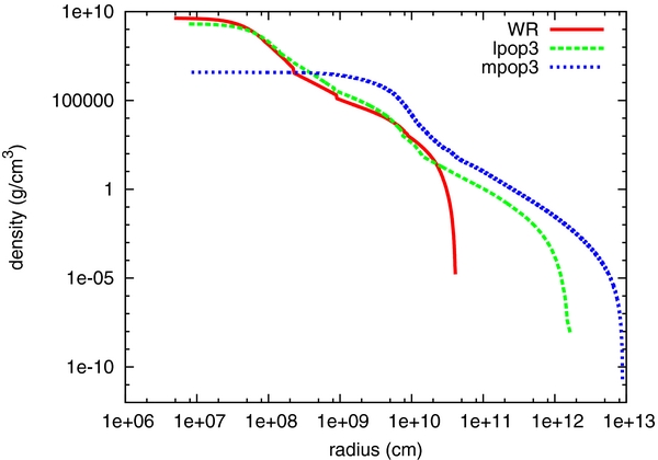
Figure 1. Density profiles of the progenitor models used in this paper (see Table 1).
Download figure:
Standard image High-resolution imageTable 1. Summary of Stellar Models
| Progenitor Model | Total Mass | Stellar Radius |
|---|---|---|
| (M☉) | (cm) | |
| W-R | 14 | 4 × 10¹⁰ |
| lpop3 | 40 | 1.5 × 10¹² |
| mpop3 | 915 | 9 × 10¹² |
Notes. (1) Wolf-Rayet star (16TI in Woosley & Heger 2006, W-R), (2) light Pop III star (Woosley et al. 2002, lpop3), (3) massive Pop III star (Ohkubo et al. 2009, mpop3).
Download table as: ASCIITypeset image
We map the spherical symmetric progenitors into two-dimensional grids in spherical coordinates. The computational domain for each stellar progenitor covers from a certain inner radius to the stellar surface. Although the inner boundary should be located in the vicinity of a black hole (around 106–107cm), this is computationally very expensive, so we set the inner boundary far from a black hole. For our reference models, the inner boundary for each progenitor is located at Rin ∼ 10−2 × Rstar, where Rstar denotes the stellar radius (see Table 2). According to this limitation, our discussions in the present paper are at the qualitative level. The outer boundary for each model is set in slightly outside from each progenitor. It is located at 4 × 1010 cm, 1.7 × 1012 cm, and 1013 cm for W-R, lpop3, and mpop3, respectively. For all models, the number of standard radial grid points is 500. The grid width is non-uniform and increasing in geometric progression (Nagakura et al. 2011). The innermost grid width is set as Δr = Rin/10, where Rin is the radius of the inner boundary from the center. Then, the rate of geometrical increase is determined so as to cover all computational regions with 500 meshes. The angular grid covers a quadrant of the meridian section (where we assume equatorial symmetry) and is uniform with 60 grid points. We employ an adaptive mesh refinement (AMR) technique in order to decrease the computational cost. We deploy two levels of meshes as in Nagakura et al. (2011), where the resolution of the second level is three times finer in each direction than the first standard mesh. Thus, the angular resolution in the AMR region corresponds to 0 5 for all models. The smallest radial grid width for the W-R model is 1.6 × 107 cm, while the ones for lpop3 and mpop3 are 3.4 × 108 cm and 3.4 × 109 cm, respectively. In order to check the dependence on the resolution, we also carry out finer AMR calculations. We check calculations with five times and seven times finer AMR meshes for the W-R models (WRreso5 and WRreso7), and seven times for the other progenitor models (lpop3reso7 and mpop3reso7). For five times finer AMR meshes, the angular resolution corresponds to 03. The smallest radial grid widths are 9.6 × 106 cm (W-R), 2.0 × 108 cm (lpop3), and 2.0 × 109 cm, respectively. For seven times finer AMR meshes, the angular resolution is (3/14)°. The smallest radial grid widths are 6.9 × 106 cm (W-R), 1.5 × 108 cm (lpop3), and 1.5 × 109 cm, respectively. As we shall see in Section 3.6, the numerical resolution is important to prevent baryon pollution by numerical diffusion (although it does not affect the macroscopic jet dynamics; see Section 3.6). Note that in Table 3, the "AMR level" denotes the multiplying factor of the fine meshes.
Table 2. Summary of Our Models
| Model | Inner Boundary | Enclosed Mass | Efficiency | Half-Opening Angle | Lorentz Factor | Specific Internal Energy | Retarded Injection Time | AMR Level |
|---|---|---|---|---|---|---|---|---|
| Rin (cm) | Min(M☉) | η | θop (°) | Γj | j |
tlate (s) | ||
| WRref | 5 × 10⁸ | 2.0 | 10−3 | 9 | 400 | 10−2 | 0 | 3 |
| WRef5-4 | 5 × 10⁸ | 2.0 | 5 × 10⁻⁴ | 9 | 400 | 10−2 | 0 | 3 |
| WRef2-4 | 5 × 10⁸ | 2.0 | 2 × 10⁻⁴ | 9 | 400 | 10−2 | 0 | 3 |
| WRef1-4 | 5 × 10⁸ | 2.0 | 10−4 | 9 | 400 | 10−2 | 0 | 3 |
| WRop3 | 5 × 10⁸ | 2.0 | 10−3 | 3 | 400 | 10−2 | 0 | 3 |
| WRop6 | 5 × 10⁸ | 2.0 | 10−3 | 6 | 400 | 10−2 | 0 | 3 |
| WRop18 | 5 × 10⁸ | 2.0 | 10−3 | 18 | 400 | 10−2 | 0 | 3 |
| WRop36 | 5 × 10⁸ | 2.0 | 10−3 | 36 | 400 | 10−2 | 0 | 3 |
| WRop45 | 5 × 10⁸ | 2.0 | 10−3 | 45 | 400 | 10−2 | 0 | 3 |
| WRM3 | 5 × 10⁸ | 3.0 | 10−3 | 9 | 400 | 10−2 | 7.47 | 3 |
| WRM6 | 5 × 10⁸ | 6.0 | 10−3 | 9 | 400 | 10−2 | 26.93 | 3 |
| WRLo5 | 5 × 10⁸ | 2.0 | 10−3 | 9 | 5 | 60 | 0 | 3 |
| WRLo50 | 5 × 10⁸ | 2.0 | 10−3 | 9 | 50 | 6 | 0 | 3 |
| WRin25e8 | 2.5 × 10⁸ | 1.7 | 10−3 | 9 | 400 | 10−2 | 0 | 3 |
| WRin1e9 | 109 | 2.5 | 10−3 | 9 | 400 | 10−2 | 0 | 3 |
| WRreso5 | 5 × 10⁸ | 2.0 | 10−3 | 9 | 400 | 10−2 | 0 | 5 |
| WRreso7 | 5 × 10⁸ | 2.0 | 10−3 | 9 | 400 | 10−2 | 0 | 7 |
| WRrepr | 5 × 10⁸ | 2.3 | 10−2 | 9 | 400 | 10−2 | 1.94 | 7 |
| WRdelay | 5 × 10⁸ | 2.0 | 10−3 | 9 | 400 | 10−2 | 0 | 3 |
| lpop3ref | 1010 | 14.9 | 10−3 | 9 | 400 | 10−2 | 0 | 3 |
| lpop3ef5e-4 | 1010 | 14.9 | 5 × 10⁻⁴ | 9 | 400 | 10−2 | 0 | 3 |
| lpop3ef2e-4 | 1010 | 14.9 | 2 × 10⁻⁴ | 9 | 400 | 10−2 | 0 | 3 |
| lpop3ef1e-4 | 1010 | 14.9 | 10−4 | 9 | 400 | 10−2 | 0 | 3 |
| lpop3op3 | 1010 | 14.9 | 10−3 | 3 | 400 | 10−2 | 0 | 3 |
| lpop3op6 | 1010 | 14.9 | 10−3 | 6 | 400 | 10−2 | 0 | 3 |
| lpop3op18 | 1010 | 14.9 | 10−3 | 18 | 400 | 10−2 | 0 | 3 |
| lpop3op36 | 1010 | 14.9 | 10−3 | 36 | 400 | 10−2 | 0 | 3 |
| lpop3op45 | 1010 | 14.9 | 10−3 | 45 | 400 | 10−2 | 0 | 3 |
| lpop3in5e9 | 5 × 10⁹ | 12.0 | 10−3 | 9 | 400 | 10−2 | 0 | 3 |
| lpop3reso7 | 1010 | 14.9 | 10−3 | 9 | 400 | 10−2 | 0 | 7 |
| lpop3repr | 1010 | 15.1 | 10−2 | 9 | 400 | 10−2 | 19.9 | 7 |
| lpop3delay | 1010 | 14.9 | 10−3 | 9 | 400 | 10−2 | 0 | 3 |
| mpop3ref | 1011 | 414.4 | 10−3 | 9 | 400 | 10−2 | 0 | 3 |
| mpop3ef5e-4 | 1011 | 414.4 | 5 × 10⁻⁴ | 9 | 400 | 10−2 | 0 | 3 |
| mpop3ef2e-4 | 1011 | 414.4 | 2 × 10⁻⁴ | 9 | 400 | 10−2 | 0 | 3 |
| mpop3ef1e-4 | 1011 | 414.4 | 10−4 | 9 | 400 | 10−2 | 0 | 3 |
| mpop3op3 | 1011 | 414.4 | 10−3 | 3 | 400 | 10−2 | 0 | 3 |
| mpop3op6 | 1011 | 414.4 | 10−3 | 6 | 400 | 10−2 | 0 | 3 |
| mpop3op18 | 1011 | 414.4 | 10−3 | 18 | 400 | 10−2 | 0 | 3 |
| mpop3op36 | 1011 | 414.4 | 10−3 | 36 | 400 | 10−2 | 0 | 3 |
| mpop3op45 | 1011 | 414.4 | 10−3 | 45 | 400 | 10−2 | 0 | 3 |
| mpop3in5e10 | 5 × 10¹⁰ | 385.1 | 10−3 | 9 | 400 | 10−2 | 0 | 3 |
| mpop3reso7 | 1011 | 414.4 | 10−3 | 9 | 400 | 10−2 | 0 | 7 |
| mpop3repr | 1011 | 431.2 | 10−2 | 9 | 400 | 10−2 | 246.6 | 7 |
| mpop3delay | 1011 | 414.4 | 10−3 | 9 | 400 | 10−2 | 0 | 3 |
Download table as: ASCIITypeset image
Table 3. Summary of Our Results
| Model | Shock Breakouta | Possibility of GRB Productionb | tbrc | Einj | Edg |
|---|---|---|---|---|---|
| (s) | (1051 erg) | (1050 erg) | |||
| WRref | ○ | ○ | 8.20 | 1.67 | 5.60 |
| WRef5-4 | ○ | ○ | 11.78 | 1.23 | 3.79 |
| WRef2-4 | ○ | ○ | 37.09 | 1.71 | 2.36 |
| WRef1-4 | × | × | ... | ... | ... |
| WRop3 | ○ | ○ | 6.75 | 1.47 | 5.72 |
| WRop6 | ○ | ○ | 7.22 | 1.54 | 5.65 |
| WRop18 | ○ | ○ | 27.54 | 2.89 | 8.10 |
| WRop36 | ○ | × | 66.87 | 7.89 | 5.93 |
| WRop45 | ○ | × | 53.31 | 19.14 | 11.54 |
| WRM3 | ○ | ○ | 7.90 | 1.80 | 6.21 |
| WRM6 | ○ | ○ | 6.18 | 1.54 | 5.60 |
| WRLo5 | ○ | ○ | 8.56 | 1.72 | 5.67 |
| WRLo50 | ○ | ○ | 8.26 | 1.68 | 5.60 |
| WRin25e8 | ○ | ○ | 6.99 | 1.72 | 5.71 |
| WRin1e9 | ○ | ○ | 11.34 | 2.05 | 6.17 |
| WRreso5 | ○ | ○ | 7.63 | 1.51 | 4.27 |
| WRreso7 | ○ | ○ | 7.24 | 1.41 | 3.84 |
| WRrepr | ○ | ○ | 3.46 | 6.49 | 27.3 |
| WRdelay | ○ | ○ | 8.60 | 1.69 | 5.62 |
| lpop3ref | ○ | ○ | 288.4 | 2.89 | 11.74 |
| lpop3ef5e-4 | ○ | ○ | 454.7 | 1.90 | 7.14 |
| lpop3ef2e-4 | ○ | ▵ | 696.1 | 1.14 | 4.01 |
| lpop3ef1e-4 | ○ | ▵ | 1581.7 | 0.794 | 1.67 |
| lpop3op3 | ○ | ○ | 244.8 | 2.90 | 13.5 |
| lpop3op6 | ○ | ○ | 257.7 | 2.91 | 12.8 |
| lpop3op18 | ○ | ○ | 614.1 | 2.52 | 8.93 |
| lpop3op36 | ○ | × | 1721 | 2.44 | 6.83 |
| lpop3op45 | ○ | × | 1530.5 | 2.25 | 4.76 |
| lpop3in5e9 | ○ | ○ | 188.9 | 5.63 | 22.57 |
| lpop3reso7 | ○ | ○ | 210.5 | 2.38 | 8.72 |
| lpop3repr | ○ | ○ | 118.9 | 11.0 | 47.6 |
| lpop3delay | ○ | ○ | 306.6 | 2.94 | 11.49 |
| mpop3ref | ○ | ○ | 1219 | 127 | 463 |
| mpop3ef5-4 | ○ | ○ | 1754 | 84 | 269 |
| mpop3ef2-4 | ○ | ▵ | 7213 | 65 | 67 |
| mpop3ef1-4 | × | × | ... | ... | ... |
| mpop3op3 | ○ | ○ | 916 | 110 | 514 |
| mpop3op6 | ○ | ○ | 1002 | 116 | 501 |
| mpop3op18 | ○ | ○ | 2620 | 129 | 378 |
| mpop3op36 | ○ | × | 13427 | 344 | 319 |
| mpop3op45 | ○ | × | 12263 | 327 | 289 |
| mpop3in5e10 | ○ | ○ | 929 | 147 | 572 |
| mpop3reso7 | ○ | ○ | 1197 | 124 | 410 |
| mpop3repr | ○ | ○ | 563 | 556 | 2437 |
| mpop3delay | ○ | ○ | 1218 | 125 | 475 |
Notes. a○: Success of shock breakout, ×: failure of shock breakout. b○: there is a possibility of GRBs, ▵: touchy to judge the possibility of GRBs, ×: there is no possibilities of GRBs. cTime at shock breakout. This time is measured from the beginning of central engine.
Download table as: ASCIITypeset image
We assume that the central engine successfully operates and the well-confined outflows are produced in the vicinity of a black hole. We inject the plasma in the radial direction through the inner boundary with an opening angle of several degrees. In this paper, we also assume that the jet luminosity depends only on the accretion rate which is estimated by the mass flows across through the inner boundary:
where rin and vr denote the location of the inner boundary and the radial velocity of flows. We inject an outflow with a luminosity

where η and c denote the accretion-to-jet conversion efficiency parameter and the speed of light, respectively. The maximum conversion efficiency as a consequence of the accretion process is 5.7% for a Schwarzschild black hole and 42% for an extreme Kerr black hole (Shapiro & Teukolsky 1983). Thus, we choose the value of η less than that. The conversion efficiency, jet opening angle, specific internal energy, and radial velocity are varied in each model. Once these parameters are fixed, the density and pressure of injected jets are determined by using the relation

where h(≡ 1 + /c2 + p/(ρ0c2)) and ΔS denotes the specific enthalpy and the area of the injection surface, respectively.
The collapse of the massive envelope is induced in the same way as in Nagakura et al. (2011). In reality, the stellar envelope begins to fall after the arrival of a rarefaction wave that is generated by the inner core collapse. We mimic this situation by setting the radial gradient of all quantities to zero at the inner boundary except for the jet injected regions. At the beginning of the simulation, the break of the force balance at the inner boundary induces the infall of matter. Subsequently, a rarefaction wave propagates outward, inducing the infall as it reaches each point. It should be noted, however, that the stellar progenitors used in this paper, especially the W-R progenitor, are not exactly in dynamical equilibrium, in contrast to Nagakura et al. (2011). Accordingly, the outer parts of the envelope begin to move and several artificial waves are observed during the simulations. We find that they induce artificial explosions in some models (but only for non-successful shock breakout models). This is because the W-R stellar model, for example, originally involves rotation (see, e.g., Woosley & Heger 2006), so that the centrifugal force works to sustain the stellar configurations. Since we artificially remove rotation, the envelope tends to infall and induce artificial compressions and bounces. We note that even the original 16TI model is not in exact dynamical equilibrium. Contrary to Nagakura et al. (2011), we do not take special treatments for the initial stellar configurations here.
We also investigate the dependence on the timing of the jet injection, since we still have a few constraints on the starting time of the central engine. If the operation of the central engine is sufficiently late, the density profile of the stellar envelope is changed by the accretion. Thus, it is expected that the jet dynamics also depends on the timing of the jet injection. In addition, we would like to investigate whether the later jet can really accomplish the shock breakout since the large mass accretion may prevent the jet propagations in this case. Motivated by these facts, we initially let the stellar envelope spherically collapse, and then inject a relativistic jet. We carry out these simulations only in W-R models because the enclosed mass at the inner boundary for our reference model is Min ∼ 2 M☉, which may be lower than the critical mass of the black hole formation (Demorest et al. 2010). As a result, it is quite likely that the central engine does not operate for a while. On the other hand, the Pop III models have so much mass enclosed at the inner boundary (see Table 2) that the central engine would begin to work soon after the collapse in our models. We prepare two models, WRM3 and WRM6, which inject the jet when the enclosed mass at the inner boundary reaches Min = 3 M☉ and 6 M☉, respectively. The corresponding retarded time of injection for each model is tlate = 7.47 s and 26.93 s, respectively. The radial density profiles just before the jet injection are displayed in Figure 2 for these models.
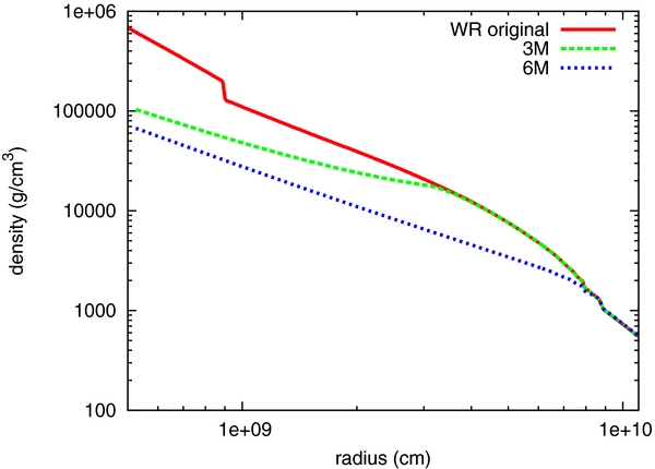
Figure 2. Radial density profile for the late time injection models. The red line is the original stellar profile of the W-R model while the green (blue) line indicates the density profile at the time when the enclosed mass at the inner boundary becomes M = 3 M☉ (M = 6 M☉) as a result of the spherical collapse. The rarefaction waves can be clearly seen in this figure.
Download figure:
Standard image High-resolution imageAll of our models used in this paper are summarized in Table 2. We prepare a reference model for each progenitor with the following parameters. The inner boundary is located at Rin ∼ 10−2 × Rstar, where Rstar denotes the stellar radius. The accretion-to-jet conversion efficiency (η), half-opening angle of outflows (θop), injected Lorentz factor (Γj), and injected specific internal energy (j) are set as η = 10−3, θop = 9°, Γj = 400, and j = 10−2, respectively. Note that these models assume that the injected jet has already reached the terminal Lorentz factor. It may not be true for W-R models since the inner boundary is located somewhat closer to the black hole than the other progenitor models. However, as we shall see, if the choice of the terminal Lorentz factor is the same, the overall profiles of jet dynamics do not depend on whether the jet injection is kinetic dominant or thermal dominant (we demonstrate Γj = 5, 50 cases in WRLo5 and WRLo50 models). In order to study the dependence on the accretion-to-jet conversion efficiency, we vary it as η = 5 × 10⁻⁴, 2 × 10⁻⁴, and 10−4 (models such as WRef..., lpop3ef..., mpop3ef...), while other parameters are identical to the reference model. We also study the dependence on the half-opening angle with θop = 3°, 6°, 18°, 36°, and 45°. The study for the injection timing is done only in W-R progenitor as WRM3 and WRM6 models. As we have already mentioned, we check the dependence on the location of the inner boundary (models such as WRin..., lpop3in..., mpop3in...) and we also conduct resolution checks (models such as WRreso..., lpop3reso..., mpop3reso...).
According to these studies, we find favorable conditions for creating GRBs. In consideration of these results, we also perform numerical simulations with representative parameters (models such as WRrepr, lpop3repr, mpop3repr). As shown in the following section, representative models succeed a powerful relativistic jet breakout and they are the most guaranteed candidates to create GRBs in our models.
3. RESULT AND ANALYSIS
In this section, we describe the numerical results obtained from our hydrodynamic simulations and analyze them in detail. We first explain overall features of the jet dynamics, and then we further analyze the dependence on each parameter and model. We also present simple analytic criteria for the possibility of GRB production at the end.
3.1. Basic Feature
We summarize numerical results in Table 3. Here, we define the shock breakout as that the forward shock wave successfully reaches the stellar surface. It should be noted, however, that shock breakout is a minimal requirement for producing GRBs. As we shall see, even if the outflow successfully accomplishes the breakout, some models are not suitable for GRBs (see the column "Possibility of GRB production" in Table 3). We assess the possibility of GRB production by the diagnostic terminal Lorentz factor Γdt ≡ h × Γ profiles on the z-axis at the time of the shock breakout. (Note that the diagnostic terminal Lorentz factor is the achievable Lorentz factor after the internal energy is converted into kinetic energy.) If there are regions where Γdt ⩾ 100 is satisfied, we determine that the model has a potential to produce GRBs. If this condition is not satisfied, the jet is not successfully injected or does not move forward. As a result, the explosion would never become relativistic enough. Note that some models are hard to judge for the possibility of GRB production because of several reasons (see the column "Possibility of GRB production" in Table 3 where we denote these models by ▵; see also the discussion in Section 3.6). The details of these models are presented in the following subsections. One of the remarkable results in this study is that many models successfully accomplish relativistic shock breakout even though the progenitor star has an extremely large envelope such as Pop III stars. These results are the numerical verification of Suwa & Ioka (2011). We will further analyze the dependencies on the efficiency η and the opening angle θop in the following section. Indeed, the jet dynamics strongly depend on these key parameters.
At the beginning of the simulations, the infall starts at the innermost regions and subsequently a rarefaction wave propagates outward. The accretion rate increases with time and then the injected energy generates the forward shock wave around the polar regions. It should be noted, however, that the forward shock wave does not propagate outward into the active computational regions for a while because of the interruption by the infalling matter. If the injected energy is not enough to push the infalling stellar mantle aside, the mantle advects inward and eventually it is swallowed into a black hole. As a result, the total amount of explosion energy becomes less than the injected energy. Furthermore, the binding energy by a black hole (and also the progenitor star itself) further reduces the explosion energy. We also calculate the diagnostic energy Edg at the time of the shock breakout in each model and show them in the fifth row of Table 3. We define the diagnostic energy Edg as the integral of lc (local energy density), which is the sum of the internal, kinetic, and gravitational energy densities, over the regions with positive lc and vr. Note that Edg is not the isotropic energy but collimation-corrected true energy. In the weak gravitational field limit, we can define lc as

where Ttt and ψ denote the time–time component of the energy momentum tensor and gravitational potential, respectively. Note that, for this definition of diagnostic energy density, gravity is treated as an external force. This estimation is valid only when the central core object takes the dominant role for gravity. If the outer envelope plays an important role for gravitational energy, we need to take into account self-gravity. So, the term of the gravitational energy should be contributed not in the form of ρ0ψ but  in Equation (4). However, since we use this value for diagnosing whether or not the outflow is relativistic in this study, the severe definition of this quantity is not necessary. Thus, we use Equation (4) in the present paper. As can be seen in Table 3, we find that the diagnostic energy for all models is less than about a third of the injected energy. Thus, it implies that the central engine has to produce a larger amount of energy than that observed as GRBs.
The total amount of explosion energy would be larger than the diagnostic energy Edg at the breakout since the central engine is able to keep operating after the shock breakout due to the continuing accretion. Indeed, as we shall see in the following subsections, some models are active at the time of the breakout. Thus, although Edg may be lower than the typical GRB energy in some models, the outflows would gain further energy from the central engine to create GRBs after the breakout.
When the injected energy is successfully launched from the inner boundary, some portions of matter bounce back and move outward. However, we cannot see a clear collimated outflow at the beginning of the simulations even if we inject dominant kinetic outflows in a small opening angle. This is due to the fact that the injected energy is thermalized by the strong reverse shock wave in the vicinity of the inner boundary. As a result, the hot matter expands and creates a quasi-spherical forward shock wave. Nevertheless, we find that the forward shock wave is not strong enough to stop the infall of matter around the equatorial region and the matter continues to accrete through the inner boundary (see, e.g., Figures 3 and 5). The jet structure emerges when the injected energy becomes enough to push away the reverse shock wave outside the computational region. Subsequent evolution is similar to the previous studies of jet propagation. The hot cocoons cause recollimation shock waves, and strong backflows also appear in the flows and they sometimes pinch the jet. The Kelvin–Helmholtz instability also works to create rich internal structures. The jet starts to propagate and the forward shock wave eventually breaks out of the stellar surface.

Figure 3. Time evolutions of inner core mass (black hole mass) for each model.
Download figure:
Standard image High-resolution image3.2. Dependence on the Accretion-to-Jet Conversion Efficiency η
As shown in Table 3, we find that the forward shock wave can break out if the accretion-to-jet conversion efficiency is η ≳ 10−4 (see more details in the Section 3.7). Figure 4 displays the time evolution of the radius for the forward shock wave on the z-axis for models with different efficiencies. As expected, the higher conversion efficiency generates a stronger shock wave, which quickly propagates into the stellar envelope. In the case of lower conversion efficiency models, however, it is harder to inject the jet. Even if the jet is successfully injected, it takes a longer time for the forward shock wave to reach the stellar surface than in the high-efficiency models.
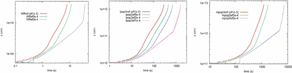
Figure 4. Time evolutions of forward shock waves on the z-axis for different accretion-to-jet conversion efficiency η models. Left: W-R models. Middle: lpop3 models. Right: mpop3 models. Note that at the beginning of simulations, the artificial oscillations arise due to the difficulty of identification of shock position. However, they do not affect our main results.
Download figure:
Standard image High-resolution imageFigure 5 shows the time evolution of the accretion rate and luminosity in these models (note that we also display the results for the failed models without breakouts). At the initial phase, the higher efficiency models have slightly smaller accretion rates than the lower efficiency models because the strong outflows interrupt the infall of matter. Still, the high-efficiency models have higher jet luminosity than the low-efficiency models. As a result, the jet successfully gains energy from the central engine and accomplishes the shock breakout. It is also interesting to note that low-efficiency models often show rapid time variability of the accretion rate (see, e.g., WRef2e-4 model in the upper left panel in Figure 5). This is attributed to the fallback of the shocked envelope, which has rich internal structures. Although the envelope initially expands due to the deposited energy, they do not have enough energy to keep moving outward and they eventually fall back through the inner boundary, leading to the central engine activity.
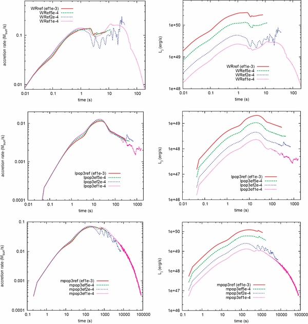
Figure 5. Time evolution of accretion rate (left) and luminosity (right) for different accretion-to-jet conversion efficiency η models. The upper, middle, and bottom panels show the W-R models, lpop3 models, and mpop3 models, respectively.
Download figure:
Standard image High-resolution imageFigure 6 shows the map of regions with positive lc and vr at the time of the shock breakout. We can see that the shape of the yellow region, which contains both positive lc and vr (see Equation (4)), does not depend on the accretion-to-jet conversion efficiency η so much. Irrespective of η, the maximum transverse radii of the yellow region from the z-axis are ∼5 × 109 cm, ∼2 × 1011 cm, and ∼1.5 × 1012 cm for the W-R, lpop3, and mpop3 models, respectively. It may imply that the outflow structure does not mainly depend on the efficiency η, as long as the shock breakout occurs (see also the next subsection). From this figure, we can also confirm that even the large efficiency jet does not expel all portions of the stellar mantle, and matter can continue to accrete onto the black hole. On the other hand, the inner parts of the envelope profiles depend on the efficiency η. As expected, a larger amount of matter is captured for the lower conversion efficiency. In addition, as discussed above, the fallback of matter causes the late time variability of the central engine.
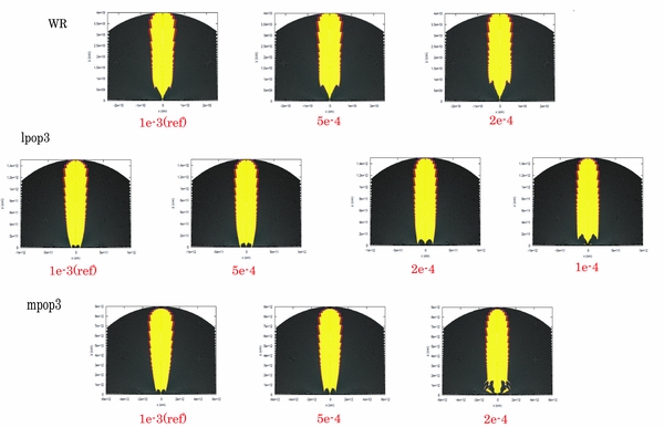
Figure 6. Regions with positive lc and vr (yellow) at the time of the shock breakout for different accretion-to-jet conversion efficiency η models (see Section 3.1 for the definition of lc and vr). The upper, middle, and bottom panels show the W-R models, lpop3 models, and mpop3 models, respectively.
Download figure:
Standard image High-resolution imageIn Figure 7, we show Γdt profiles along the z-axis at the time of the shock breakout for each model. The model has the potential to produce a GRB if Γdt ⩾ 100 is satisfied in some region. Therefore, we use this condition to assess whether or not the model can create a GRB. We note that the reality is more complex as argued in the following. In Figure 7, the outer region tends to contain lower values of Γdt, even less than ∼10. The small Γdt is caused by the baryon pollution in the jet, most likely because of the lack of numerical resolution (see in Section 3.6). However, even if the baryon pollution were the real physical phenomenon, these outflows would create GRBs for the high-efficiency models (η = 10−3) because the central engine keeps operating after the shock breakout for these models (see discussions in Section 3.6). The inner fast-moving jets would eventually catch up with the slowly moving outer ejecta. Due to this energy input from the inner jets, it is quite likely that the actual terminal Lorentz factor of the outer outflows is larger than the values of the current estimation. Thus, we expect relativistic explosions in these models. However, it is less likely that the low-efficiency models such as lpop3ef-4, lpop3ef2-4, and mpop3ef2-4 can successfully gain energy from later jets. Even if the central engine keeps operating for a long time, they may not be able to accelerate outflows because the amount of the outer slow matter is large (the profile of Γdt deviates from the high-efficiency models) in these models. As a result, the energy of the jet is dissipated in the vicinity of the injection region without transferring the energy into the outer parts of the ejecta. According to this consideration, we regard that these low-efficiency models would end up with non-relativistic explosions and may not create GRBs (thus, we mark these models with triangles (▵) in the column "Possibility of GRB" in Table 3.) We note that if the reverse shock is stalled near the injection region at the time of the shock breakout, there is no hope for this reverse shock to go ahead afterward because the accretion rate is decreasing.
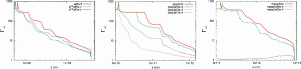
Figure 7. Diagnostic terminal Lorentz factor profile (Γdt ≡ h × Γ, i.e., the Lorentz factor which the jet can in principle attain) at the time of the shock breakout for different accretion-to-jet conversion efficiency η models. From left to right, W-R models, lpop3 models, and mpop3 models, respectively.
Download figure:
Standard image High-resolution image3.3. Dependence on Opening Angle θop
Figure 8 shows the time evolution of the forward shock wave on the z-axis for models with different opening angles of the jet at the injection site. Generally, the forward shock wave propagates fast and succeeds in breaking out if the opening angle is small. It is mainly attributed to two reasons: one reason is that the isotropic flux is increased by the small cross-sectional area of the injected jet, and the other is the increment of the accretion rate. A wide opening angle tends to interrupt the accretions and reduce the jet luminosity (see Figure 9).

Figure 8. Time evolutions of forward shock waves on the z-axis for different opening angle θop models. From left to right, we show the W-R models, lpop3 models, and mpop3 models, respectively.
Download figure:
Standard image High-resolution image
Figure 9. Time evolution of the accretion rate (left) and the luminosity (right) for different opening angle θop models. The upper, middle, and bottom panels show the W-R models, lpop3 models, and mpop3 models, respectively.
Download figure:
Standard image High-resolution imageNote that the overall dynamics for very wide opening angle jets (e.g., θop = 36 and 45°) are more complex than the collimated jets. As shown in Figure 8, the jet breakout time for θop = 45° models are (slightly) earlier than θop = 36° models in all types of progenitors. It is because the fallback process plays an important role for wider jets by enhancing the accretion rate. Indeed, for WRop45, the accretion rate reaches  at t = 45 s, and leads to the strong outflows from the inner boundary and finally to the shock breakout. Thus, the late time activity of the central engine is possible for a wide opening angle due to the strong fallback accretions, even though the mean accretion rate decreases with time in the late phase. (But these wide opening angle jets are not suitable to produce relativistic outflows; see below.)
In Figure 10, we display the time evolution of the forward shock wave for different angle radial rays from the symmetry axis. For reference models (left panels in this figure), the forward shock velocity decreases with increasing angle. Particularly, at the time of the shock breakout, we find that the forward shock waves along the off-axis radial ray are still deep inside the star, which means that the outflow is well collimated. On the other hand, for θop = 36° models, almost all models experience quasi-spherical evolutions. Although the shock wave on the z-axis is slightly faster than the off-axis shock waves, it is much more spherical than the reference model at the breakout. As a result, it is expected that the wide opening angle models never create GRBs in view of the spherical morphology of the outflows.
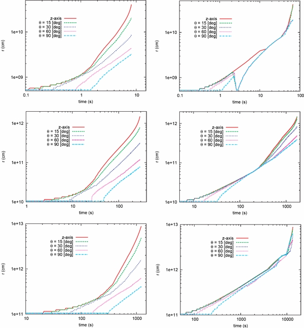
Figure 10. Forward shock evolution along each radial ray with different angles from the axisymmetric axis. We show two different opening angle jet models. Left: reference model (θop = 9°), right: (θop = 36° model). From upper to lower panels, we show the W-R, lpop3, and mpop3 models, respectively.
Download figure:
Standard image High-resolution imageFigure 11 is the same as Figure 6, but for models with different opening angles. We do not find any clear differences for narrow opening angle jet models (θop = 3° and 6°), so we do not display these models in this figure. As shown in this figure, the wider jet tends to expel a larger outer envelope, and clearly these profiles are different from each other. Also, we again see that very wide angle cases are very complicated. Interestingly, some fraction of stellar mantle around the equatorial region may never fall back to the black hole (see the θop ⩾ 36° models). From what has been discussed above, we can conclude that the outflow profile is mainly determined by the opening angle of the jet θop rather than the accretion-to-jet conversion efficiency η (see also Figure 6 and discussions in Section 3.2).

Figure 11. Same as Figure 6 but for different opening angles.
Download figure:
Standard image High-resolution imageThe diagnostic terminal Lorentz factor profiles along the z-axis for different opening angle models are shown in Figure 12. For small opening angle models (θop ⩽ 9°), the diagnostic terminal Lorentz factor is very much not different (slightly larger value for wider opening angle). However, the profile of very wide models is completely different from narrow jet cases and the terminal Lorentz factor for the wide angle models is quite low. Thus, they are no longer capable of producing GRBs. Note that, although the jet of mpop3op36 model is successfully injected around the inner boundary (see in Figure 12), this outflow may not create GRBs since the outer ejecta is completely non-relativistic, Γdt ∼ 1, and the outflow configuration is not collimated. As a result, a small opening angle θop ≲ 20° is necessary for relativistic shock breakout and GRBs with the case η ∼ 10−3. Note that if the efficiency becomes lower than η = 10−3, the opening angle needs to be smaller than the current value, because it is harder for the low-efficiency jet to push aside the infall matter than the high-efficiency jet (see Section 3.7 for the analytic estimation of the breakout criteria).

Figure 12. Same as Figure 7 but for different opening angles.
Download figure:
Standard image High-resolution image3.4. Dependence on Injection Lorentz Factor Γj and Injection Timing tlate
In this section, we discuss how the injection Lorentz factor and the jet injection timing affect the evolution of the jet. In Figure 13, we display time evolutions of some key quantities, such as the forward shock wave on the z-axis, the mass accretion rate, and the jet luminosity. As we can see, the injection Lorentz factor does not change the qualitative feature of the jet evolutions for all quantities as long as the final coasting Lorentz factor is the same (see the left panels in Figure 13).
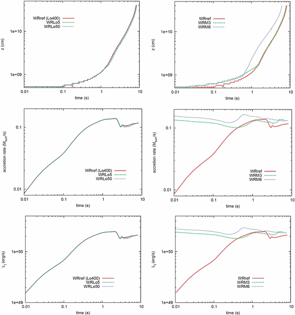
Figure 13. Dependence on the injection Lorentz factor and the timing of the jet injection. Left: different injection Lorentz factor, right: different injection timing. Upper to lower: the time evolutions for the shock evolution along the z-axis, the mass accretion rate, and the jet luminosity, respectively.
Download figure:
Standard image High-resolution imageOn the other hand, the jet dynamics depend on the timing of the jet injection (see the right panels in Figure 13). We can see that late injection leads to a slightly faster evolution than early injection, and also that the time evolution of the accretion rate and the jet luminosity are quite different in the early phase. This is because the accretion rate is already high at the time of the jet injection for the late injection. As a result, the strong jet is injected and evolves faster than the early injection case. It should be noted that although the late jet injection slightly interrupts the infall of the material (see the middle and right panels of Figure 13), it does not stop the accretion of all the infalling material. We also speculate that a wide opening angle would suppress the infall of matter more strongly, so that the collimated outflows are preferred for GRBs even in the late injection cases.
It is also interesting to investigate the diagnostic terminal Lorentz factor Γdt profile for the different timings of jet injection as displayed in Figure 14. As we can see in this figure, the late jet injection tends to have a higher diagnostic terminal Lorentz factor than the early jet injection. This is also because the jet luminosity for the later injection case is stronger than the earlier jet (see the bottom panel of Figure 13). The strong forward shock waves propagate outward and the outer envelope obtains a large amount of energy from them. Besides, we also find that the late jet injection tends to have a smaller amount of baryon mass in the jet since a portion of envelope matter has already been swallowed in the black hole. As a result, the outflow easily achieves relativistic velocity after the breakout (see Table 4 and Section 3.6 for more details). We again must caution that the artificial baryon pollution affects the distribution of the diagnostic terminal Lorentz factor and the amount of baryon mass. The detailed discussions of these issues are described in Section 3.6. Note also that too late an injection may not be suitable for GRBs, since the accretion rate becomes very low and centrifugal bounce takes place at a later time (see Nagakura et al. 2011). Although we do not know exactly the starting time of the central engine, we speculate that the most plausible starting timing for the central engine is the time when the accretion disk is formed around a black hole. It clearly depends on the angular momentum distribution of the progenitor star, so we will investigate this dependence by performing the rotational collapse of progenitor stars in a forthcoming paper (H. Nagakura et al. 2012, in preparation).

Figure 14. Same as Figure 7, but with a different timing of the jet injection.
Download figure:
Standard image High-resolution imageTable 4. The Baryon Mass and Final Lorentz Factor for Jets
| Model | Baryon Massa | Jet Energyb | Average Terminal Lorentz factorc |
|---|---|---|---|
| (M☉) | (Ej) | (Γf) | |
| WRref | 9.25 × 10⁻⁵ | 9.43 × 1051 | 57 |
| WRreso5 | 5.36 × 10⁻⁵ | 9.70 × 1051 | 101 |
| WRreso7 | 2.61 × 10⁻⁵ | 9.78 × 1051 | 209 |
| WRM3 | 7.43 × 10⁻⁵ | 8.42 × 1051 | 63 |
| WRM6 | 4.57 × 10⁻⁵ | 5.73 × 1051 | 70 |
| WRrepr | 2.52 × 10⁻⁵ | 9.17 × 1052 | 2035 |
Notes. aThe baryon mass contained in the jet at the breakout. See Equation (5) in Section 3.6 for its definition. bThe total energy of the injected jet after the breakout. cThe average terminal Lorentz factor of outflows estimated by Equation (7).
Download table as: ASCIITypeset image
3.5. Representative Models
Based on the above results, we construct representative models, which are expected to create GRBs in each progenitor. As we have seen, the favorable conditions for relativistic shock breakout are high conversion efficiency, small opening angle, and late jet injection. We summarize these parameters for representative models in Table 2. We denote these representative models as WRrepr for the W-R progenitor, lpop3repr for the light Pop III star, and mpop3repr for the massive Pop III star. The accretion-to-jet conversion efficiency is set as η = 10−2 which corresponds to nearly the maximum conversion efficiency for a Schwarzschild black hole (see Section 2). The half-opening angle is set as θop = 9°. We start to inject the jet when the mass accretion rate becomes the largest for each progenitor. We also note that we carry out simulations with higher spatial resolutions (seven-level AMR) in order to suppress the artificial baryon pollutions (see in Section 3.6 for more details).
We summarize numerical results in Table 3. As you can see in this table, the forward shock wave propagates faster than the reference model. We also find that both the total amount of injection energy and diagnostic energy at the breakout time are larger than those of reference models. Figure 15 shows the Γdt distribution along the jet axis at the shock breakout for each model. As can be seen in this figure, every model produces more relativistic breakout than the corresponding reference models. In particular, it is interesting to note that mpop3repr succeeds with highly relativistic breakout in spite of a large massive envelope. Note that the outer ejecta for WRrepr and lpop3repr is still mildly relativistic (Γdt ∼ 30). This is most likely caused by the numerical baryon contamination. However, even if the baryon pollution were real, these outflows could accelerate relativistically and create GRBs for the same reason discussed in Section 3.2 (see also Section 3.6).
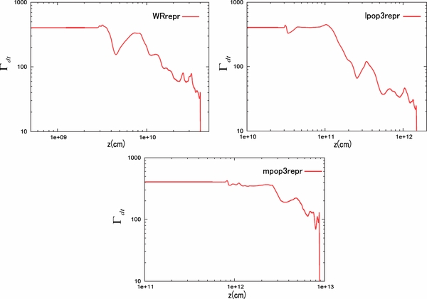
Figure 15. Same as Figure 7, but for representative models.
Download figure:
Standard image High-resolution image3.6. Limitation of the Current Study
In this subsection, we give some important cautions for the results presented in this paper. Although our simplification of numerical methods does not change the essence of our new findings, there are some technical limitations for the current numerical simulations. Here, we point out several limitations on the present work with some additional simulation results.
3.6.1. Baryon Pollution
Although our numerical code succeeds in capturing strong shock waves and complex turbulence in relativistic outflows, numerical diffusion is inevitably inherent in it. As a result, numerical diffusion potentially induces artificial baryon pollution which leads to a lower diagnostic terminal Lorentz factor in the jet. As we have already mentioned, since Γdt is important in determining whether or not the jet would eventually create a strong relativistic outflow, we need to know how the numerical resolution affects Γdt along the jet axis.
Figure 16 shows the comparison of Γdt distribution along the jet axis for models with different spatial resolutions. As you can see in this figure, models with higher resolution exhibit a larger Γdt. This confirms that higher resolution reduces the baryon pollution and shows the higher value of Γdt. In fact, the amount of baryon mass around the jet axis at the breakout time is decreasing with higher resolutions (see Table 4). The baryon mass contained in the jet is roughly estimated as

where ρz(r) denotes the density profile along the z-axis. We also estimate the average terminal Lorentz factor Γf for the jet as
where Ej denotes the total injected energy after the breakout. We estimate Ej as

where Mbound denotes the total mass of gravitationally bound matter (see also Equation (4) for the definition of bound matter). Here, we assume that all of energy from the central engine is successfully transferred to outgoing ejecta. As shown in Table 4, the outflow for WRref can accelerate Γf ∼ 60 although this model is heavily influenced by the baryon pollution. Thus, even if baryon pollution were occurring in reality, this model could create relativistic outflow. In addition, we would like to emphasize that the macroscopic jet evolution is not sensitive to the numerical resolution (see Figure 17).
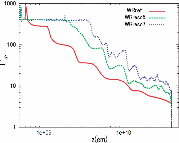
Figure 16. Same as Figure 7, but with different spatial resolutions among W-R models (WRref, WRreso5, and WRreso7).
Download figure:
Standard image High-resolution image
Figure 17. Dependence on the resolutions of our simulations. Left: the forward shock evolution along the z-axis, right: the time evolutions of the luminosity.
Download figure:
Standard image High-resolution imageWe also point out that the two-dimensional axisymmetric setup affects baryon pollution. In our simulations, the baryon pollution near the pole is mainly attributed by the numerical diffusion, since the meridian velocity near the pole is almost zero due to the axisymmetric property. However, in reality, non-axisymmetric motions and finite meridian velocity may happen in the jet region. In this case, there is a possibility that the cocoon or strong back flows thrust into jets, then a lot of baryons could mix with the jet matter. Note also that the dense "plug" at the head of the jet is an artifact of the axisymmetric property. In reality, the non-axisymmetric motions of jet would cause dispersion of the dense "plug" (Zhang et al. 2004).
3.6.2. Dependence on Inner Boundary Location
One of the other drawbacks in the present study is the choice of inner boundaries in current models. For all simulations, the inner boundary is located well outside the central core of the star. As a result, the mass accretion rate for each model would be different from the actual accretion rate in the vicinity of the black hole. In addition, the impact of feedback would also be changed. In order to remove these uncertainties, we demonstrate some numerical simulations for different positions of the inner boundary.
Figure 18 shows the dependence on the inner boundaries for the evolution of the forward shock wave on the z-axis and the jet luminosities. As shown in these panels, models with a smaller inner boundary imply that the forward shock wave propagates faster. Since the density is higher at the inner radius, the accretion rate consequently becomes larger so that the jet luminosity also becomes larger. In these panels, we find that the model lpop3in5e9 has a peak accretion rate of about 10 times that of model lpop3ref, while W-R and mpop3 simulations exhibit only a factor of two or three amplification, when the inner boundary is smaller by a factor of two. We also note that, for the mpop3 models, the initial enclosed mass at the inner boundary is 414 M☉ and it corresponds to nearly half the total mass of the star. Thus, the location of the inner boundary substantially affects the jet dynamics especially for lpop3 and mpop3. In order to obtain more quantitative arguments for the actual jet luminosity and breakout time, we need simulations with a smaller inner boundary, which are beyond the scope of this paper.
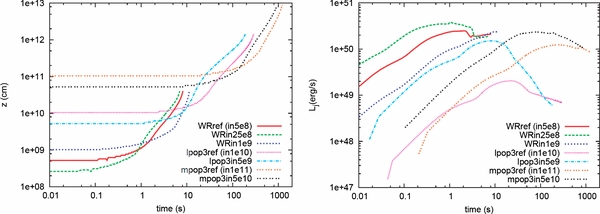
Figure 18. Dependence on the location of the inner boundary. Left: the forward shock evolution along the z-axis, right: the time evolutions of luminosity.
Download figure:
Standard image High-resolution imageIt should be noted, however, that the effect of location of the inner boundary is quite systematic: the forward shock wave becomes fast and the luminosity becomes large if we put the inner boundary on a small radius. This is probably because the density is initially higher near the boundary. Consequently the total mass accretion rate increases and therefore the jet luminosity becomes large with a strong forward shock wave. According to these results, it is a robust claim that the shock breakout is possible if the accretion-to-jet conversion efficiency satisfies the condition η ≳ 10−4 (see more details in Section 3.7).
3.6.3. The Time Delay between Infall and Injection
In the present study, we assume that the jet outflow is injected immediately after the mass inflows through the inner boundary. However, it takes a certain amount of time for the fluid to reach the vicinity of the black hole in reality. In addition, the outflow should travel up to the inner boundary. The time difference can be roughly estimated based on the assumption that the matter free falls to a black hole. At the beginning of our simulation, it takes ∼1 s for the W-R model from the inner boundary to the center of the core, while ∼20 s and ∼150 s for lpop3 and mpop3, respectively. Our immediate energy injection would be different from reality and potentially affects our findings. Here, we investigate the influence of the time delay between infall and jet injection.
We perform numerical simulations for some models, taking into account the delay time of the jet injection. In this study, we estimate the delay time as free-fall time from the location of the inner boundary to the Schwarzschild radius. Note that the Schwarzschild radius is estimated by the enclosed mass at the inner boundary. We ignore the jet propagation time from the vicinity of the black hole to the location of the inner boundary. This is because the timescale of jet propagation is much less than the free-fall time. The jet injection parameters, such as the conversion efficiency and opening angles, are the same as the reference models. Hereafter, we denote these models as WRdelay, lpop3delay, and mpop3delay for the W-R, lpop3, and mpop3 progenitors, respectively.
In Table 3, we show the summary of results for these models. In comparison with reference models, the overall dynamics are qualitatively similar to those of reference models. In addition, the variation of the breakout time, the total injection energy, and the diagnostic energy remain within 10% from those of reference models. Thus we confirm that the time delay between infall and injection is a minor effect. This seems to be attributed to the fact that the accretion rate is almost constant except for at the very early phase of collapse. As a result, the delayed time injected jet goes through comparable ram pressure to the non-delayed injection case. Therefore, the forward shock evolution is similar to the reference models.
3.6.4. Long-term Simulations
In the current study, we investigate the jet propagation inside the stellar mantle and discuss the possibility of GRBs. However, in order to know how these outflows accelerate in the interstellar medium (ISM), it is necessary to carry out simulations with longer duration and a large spatial region. Although our simulations have a limited duration and spatial extent, we perform extended numerical simulations for the W-R reference model for the purpose of qualitative understanding of the outflow properties. We extend the computational boundary to r ∼ 5Rstar and carry out the simulation until the forward shock wave reaches the outer boundary. We cover 1500 uniform radial grids in this extended spatial region, i.e., the total number of our radial grids are 2000 (500 + 1500). The grid width is the same as the outermost radial width of previous calculations. The outer boundary in this calculation is located at rout = 2.34 × 1011 cm. In this simulation, the three-level AMR technique is employed. Thus, the radial resolution in the extended region corresponds to Δr = 4.27 × 107 cm. The meridian grid width is the same as previous calculations.
Figure 19 shows some snapshots for the diagnostic terminal Lorentz factor distribution along jet axis. As we can see in this figure, the outflow propagates into this ISM and the inner ejecta with high Γdt gradually progresses outward with time. This is attributed to the continuous energy injection of the central engine. According to these results, even if baryon pollution were real, the outflows would continuously propagate into the ISM because it is being pushed by high Lorentz factor ejecta in the back. Note also that, since this simulation is contaminated by the artificial baryon pollution, the outflow is more relativistic in reality than this simulation. The encouraging tendencies increase the possibility of GRBs being produced in a wider range of scenarios, but future long-duration simulations are needed.
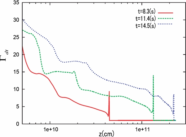
Figure 19. Same as Figure 7, but long-term simulations for WRref. The red line indicates the diagnostic terminal Lorentz factor distribution soon after the shock breakout, while the blue line indicates the same distribution but t = 14.5(s) which is the final time of this simulation. The snapshot for green line (t = 11.4(s)) corresponds to the middle time between them.
Download figure:
Standard image High-resolution imageIn summary of this subsection, in order to judge whether the outflows become relativistic or not in reality, we need to simulate them with (1) high resolution in order not to affect the baryon pollution, (2) smaller inner boundary, and (3) long duration and large spatial range. Here, we emphasize that the results of the current study give conservative claims for the possibility of relativistic jet breakout, which is the minimum requirement for producing GRBs. In fact, we show that the accretion-powered jet succeeds in breaking out relativistically from massive Pop III progenitors if the adequate conditions are satisfied.
3.7. Comparison with Analytic Estimate
In this subsection, we compare our numerical results with the analytic estimate of the shock breakout in Suwa & Ioka (2011) and Appendix A.2. Since setups are rather different between the numerical study and the analytic one, we concentrate on the parameter dependence of the successful relativistic shock breakout. They derived the shock breakout time (tb; Equation (12) in their paper) and the free-fall timescale of the envelope materials, i.e., the duration of the accretion-powered jet (tff; Equation (15)). When tb is shorter than tff, the jet successfully arrives at the stellar surface and the relativistic shock breakout takes place. Employing Equations (A10) and (A11) in Appendix A.2, we can derive the criteria for the successful relativistic shock breakout as

where n (≈2.6 for mpop3 and W-R and ≈2.1 for lpop3) is an index for the density profile of the stellar envelope,
with the stellar radius R* (Matzner & McKee 1999). The prefactor λ depends on the stellar radius, the core mass, and the envelope mass, and is found to be typically around λ ∼ 3 for mpop3 according to Suwa & Ioka (2011) and Appendix A.2. In this paper, we find that λ ≈ 2 is suitable for explaining the numerical results of mpop3. The reason of the difference in λ is that some of the assumptions in Suwa & Ioka (2011) are violated, that is, they assumed a conical jet propagation (i.e., θop is independent of the radius; see Ioka et al. 2011) and neglected the negative feedback from the cocoon on the accretion rate. The breakout condition is also not exactly the same between the analytic and numerical calculations. Nevertheless, it is encouraging that both results coincide within a numerical factor.
In Figure 20, we present η − θop diagrams to compare our numerical results with the analytic criteria in Equation (8) (black solid line). The circles, triangles, and crosses in this figure correspond to the column "Possibility of GRB production" in Table 3. We use λ = 2 for all progenitor models. As we can see from Figure 20, the analytical criteria in Equation (8) and Suwa & Ioka (2011) are useful to forecast the penetrability of the relativistic jet and the possible GRB production in massive star models. We can predict the parameter space where GRBs could occur in the η − θop plane once we calibrate λ with numerical simulations. In addition, we find that the analytical critical curve can be approximated by a much simpler form for all current progenitors (W-R, mpop3, lpop3) as

Figure 20. Score sheet of the shock breakout for W-R (top panel), lpop3 (middle panel), and mpop3 (bottom panel), respectively, in the accretion-to-jet conversion efficiency η and the opening angle θop plane. Red circles correspond to the models which have possibilities for creating GRBs in our numerical simulations, while blue crosses show the failed cases. Black triangles are marginal models (see the text for details). The analytical criteria for the shock breakout in Equation (8) are shown by the black solid lines. Below this line the shock wave can break out of the stellar surface before the mass accretion ceases. On the other hand, the jet stalls inside the massive envelope and the explosion becomes spherical above this analytical line.
Download figure:
Standard image High-resolution imageNote that a red supergiant (RSG) satisfies the breakout criteria in Equation (8) with λ ∼ 6.8. Actually a GRB jet might be associated with an RSG, which has not been observed so far. A GRB from an RSG would be very dim and long because the breakout time is long due to the expanded envelope and the accretion rate is low at the late time. Such dim GRBs might even dominate as the sensitivity is improved. Alternatively, another condition could prevent the GRB production. First, the velocity of the jet head should be faster than that of the cocoon, vh > vc (Matzner 2003; Suwa & Ioka 2011). In some parameter space, an RSG does not satisfy this second criterion because of its shallow envelope and the outflow becomes almost spherical (Suwa & Ioka 2011). Second, the central engine of an RSG might not rotate fast enough for the jet production. The detailed discussion will be presented in a forthcoming paper.
4. CONCLUSIONS
In this paper, we investigate the propagation of the accretion-powered jets in Pop III and present-day stellar progenitors (W-R stars). We perform two-dimensional relativistic hydrodynamic simulations taking into account both the envelope collapse and the jet propagations for the first time. The main findings in this paper are summarized as follows.
- 1.Although some portion of matter ceases to fall and is pushed outward by the energy injection from the polar region, a large amount of matter continues accreting into the black hole, so that the central engine can continue to inject outflows.
- 2.If the central engine satisfies a certain condition (see below), the jet can successfully propagate and create a relativistic breakout from various types of progenitors for GRBs. In particular, we show that Pop III stars could be progenitor candidates for GRBs, as pointed out by Suwa & Ioka (2011). We numerically verify that the central engine can last very long, ≳ 100 s for light Pop III stars and ≳ 1000 s for massive Pop III stars because of the accretion of the huge envelope.
- 3.
- 4.We find that the timing of jet injection does not affect our results significantly. We also observe that the diagnostic terminal Lorentz factor tends to be higher for later jets than for early jet injection because the rarefaction wave reduces the central density before the strong jet is injected.
It should be noted that our simulations are affected by numerical diffusion and the location of the inner boundary as analyzed in Section 3.6. Especially for Pop III models, we put the inner boundary far outside the central core. We intend to address these issues in a future publication.
We would like to point out that the injected energy from the central engine may contribute to the explosion energy of the supernova component, if the hot cocoon mainly contributes to the supernova, i.e., an almost spherical shock wave accompanying a large amount of nickel production (see also Ramirez-Ruiz et al. 2002 for discussions of excess energy accumulated in the cocoon). If the strong reverse shock wave is still stagnant around the root of the jet at the time of the shock breakout, the kinetic energy of the jet continues to be converted into thermal energy deep inside the stellar mantle. Although the cocoon pressure would decrease after the shock breakout and make it easy for the reverse shock wave to propagate, the jet luminosity is also reduced as the accretion rate decreases, so that the reverse shock wave may stay deep inside the star. If this is the case, the injected energy may work to expel the stellar mantle rather than contribute to the GRB component. However, at the present time, it is unclear how large an amount of nickel is created in the hot cocoon, so we do not know whether the cocoon creates the supernova or not. We will address these issues in a forthcoming paper.
It is also interesting to note that if the stellar envelope consists of multi-layered configurations (i.e., an onion-like structure), the accretion rate also changes across the different layer. The change in the accretion rate may cause time variability of the central engine. The variability timescale depends on the initial location of the shell boundaries and roughly corresponds to the free-fall timescale at this region. It should be noted that stellar rotation may play an important role in this matter in a realistic situation since the specific angular momentum is also discontinuous at the shell interface, and it may cause the accretion rate to fluctuate. The angular momentum is generally an increasing function of radius in each shell, but it discontinuously drops at the shell boundary. As a result, the centrifugal force is reduced in strength there and it may potentially increase the accretion rate.
It is interesting to note that some models in the present study may explode as choked GRBs. Although they cannot produce GRBs, they are expected to produce TeV neutrinos (Mészáros & Waxman 2001). These observational signals provide important information on jet propagation in the stellar mantle. We would like to investigate the observational consequence of the different jet injection parameters in a forthcoming paper.
Finally, we would like to emphasize that the rotation profile of the stellar progenitor also affects GRB production. This is because the angular momentum profile may determine not only the starting time of the central engine but also the disk conditions (Lee & Ramirez-Ruiz 2006; Zalamea & Beloborodov 2009; Lopez-Camara et al. 2009). The dependence on angular momentum profile of progenitor is currently being investigated (H. Nagakura et al. 2012, in preparation). Additionally, there is no guarantee that the jet luminosity is proportional to the accretion rate as assumed in this paper. Actually, if the neutrino mechanism plays a key role in producing the jet, the jet luminosity also depends on the mass of the black hole. In addition, the relation between the mass accretion rate and jet luminosity in the neutrino mechanism would be different from those used in the present paper (see, e.g., Zalamea & Beloborodov 2011). These areas present the opportunity for future inquiries and are currently being investigated.
We are grateful to the anonymous referee for beneficial comments. We would also like to thank Mr. Rhosuke Hirai for useful comments and proofreadings. This work is supported in part by Grant-in-Aid for the Scientific Research from the Ministry of Education, Culture, Sports, Science and Technology (MEXT), Japan [Nos. 24740165,21684014, 19047004, 22244019, 22244030, 23840023], and by HPCI Strategic Program of Japanese MEXT, and the Center for the Promotion of Integrated Sciences (CPIS) of Sokendai.
APPENDIX
A.1. Analytic Stellar Model
Using Equation (9) of Suwa & Ioka (2011), we can calculate the stellar radius R* as
where we calibrate the overall factor to reproduce the mpop3 radius with n = 2.6. This equation is a general form of Equation (10) of Suwa & Ioka (2011). From Equation (A1), we can estimate the stellar radii of W-R, lpop3, and RSG as 8 × 1010 cm, 7 × 1011 cm, and 2 × 1013 cm, respectively, which reproduce well the actual values within a factor of two to three. In these estimations, we employ following parameters:
- 1.W-R: n = 2.6, Mc = 11 M☉, Menv = 2 M☉, and Rc = 1010 cm.
- 2.lpop3: n = 2.1, Mc = 15 M☉, Menv = 25 M☉, and Rc = 1010 cm.
- 3.RSG: n = 1.5, Mc = 4 M☉, Menv = 8 M☉, and Rc = 1012 cm.
A.2. Stellar Dependence of Breakout Criteria
In this section, we derive an analytic expression for the breakout criteria. Note that we employ typical sets of parameters to normalize physical quantities (e.g., η, θop). In order to apply this to the individual progenitor, one should insert the values from Appendix A.1.
Here, we approximate the density profile of the envelope as
in which the term of unity in Equation (9) is neglected for simplicity. This approximation is valid for r ≪ R*. The free-fall timescale of a mass shell at radius r and the enclosed mass Mr is given by
where G is the gravitational constant. The mass accretion rate is given by
where R0 is the arbitrary characteristic radius and ρ0 = ρ1(R*/R0)n. Here we neglect the derivative of Mr with respect to r for dtff/dr. Using Equation (A4), the jet luminosity emitted from the central object is written as
where tff corresponds to the jet breakout time at R0. On the other hand, the necessary luminosity for outgoing jet propagation (Suwa & Ioka 2011) is given by
Equating Equations (A5) and (A6), we get
By deleting r from Equation (A7) using Equation (A3) (i.e., r ∼ 1011 cm(Mr/250 M☉)1/3(tff/170 s)2/3), we can estimate the jet breakout time (i.e., the jet arrival time at R0) as
On the other hand, the free-fall time in Equation (A3) is
Here, we choose R0 ≈ 0.3R*, beyond which the density profile is not a power law but decreases rapidly due to the term of unity in Equation (9). The jet head accelerates due to decreasing ram pressure of the ambient matter beyond this radius. In addition, the mass accretion rate by the mass shell at r ≳ 0.3R* decreases rapidly. Therefore, we consider the critical condition for the successful jet breakout using R0 ≈ 0.3R* in the following.
By combining Equations (A8) and (A9), we obtain the criterion for the successful jet break out, which is that the free-fall timescale should be longer than the breakout timescale, as
According to the notation of Equation (8), we define λ as
For  , we replace this term with Mc + 0.4Menv to estimate the specific values (see Suwa & Ioka 2011). Using values in Appendix A.1, we find that λ ∼ 1.5, 2.6, 2.7, and 6.8 for W-R, lpop3, mpop3, and RSG, respectively.