
Abstract
The grain boundaries (GBs) of high-temperature superconductors (HTSs) intrinsically limit the maximum achievable inter-grain current density ( ), when the misalignment between the crystallographic axes of adjacent grains exceeds a certain value. A prominent effect resulting from large-angle GBs is a hysteresis of
  between the increasing and decreasing field branches. Here, we investigate this feature for K- and Co-doped Ba-122 polycrystalline bulks with systematically varied grain size and find that the widely accepted explanation for this effect—the return field of the grains—fails. We use large-area scanning Hall-probe microscopy to distinguish
  from the intra-granular current density (
 ) in order to clarify their interactions. Measurements on Ba-122 bulks reveal that a large
  results from a small
  as well as small grains. An extended version of the model proposed by Svistunov and D'yachenko is successfully applied to quantitatively evaluate this behavior. The excellent agreement between the model and experiments suggests that the GBs limit the macroscopic current in all of the samples and that the inter-grain coupling is governed by Josephson tunneling. The predictions of the model are promising in view of realizing high-field HTS magnets. Our main result is that the field dependence of the
  of an untextured wire can be significantly reduced by reducing the grain size, which results in much higher currents at high magnetic fields. This result is not limited to the investigated iron-based materials and is therefore of interest in the context of other HTS materials.
Export citation and abstract BibTeX RIS
1. Introduction
Round multifilamentary superconducting wires are the preferred choice for building high-field magnets such as those used in particle accelerators and fusion reactors [1]. Currently classic compounds, i.e. Nb–Ti and Nb3Sn, are used for these applications since wires and tapes based on high-temperature superconductor (HTS) materials are not competitive so far. Their development is closely related to the optimization of the growth process and the grain boundary (GB) properties. Great efforts have been made to reduce the misalignment between the crystallographic axes of the grains in HTSs to prevent the weak-link character of large-angle GBs and thereby increase the maximum transport current. This has been successfully achieved for HTS tapes [2], but their geometry is less preferable than the round cross section of wires and their fabrication process is complicated and expensive.
The discovery of iron-based superconductors excited much interest because of their relatively high transition temperatures, small anisotropy, and high upper critical fields  [3]. Unfortunately, measurements of the critical current density across [001]-tilt GBs in thin-film Co-doped Ba-122 bicrystals [4, 5], as well as magnetization and critical current measurements on polycrystalline iron-based compounds [6–8], indicate weakly linked GBs in these superconductors [9, 10], but their limiting effect on
  is less pronounced compared to other HTSs [4]. Recently, results on Bi-2212 wires [11] have been promising for future HTS magnet applications. The large
  of these wires is ascribed to a local biaxial texture of the grains [12]. The iron-based HTSs also have the potential for the production of superconducting wires. In contrast to Bi-2212, the wires based on Ba-122 in [13] are untextured, nonetheless, the achieved performance is much better compared to other untextured HTS wires. Still, major improvements of the iron-based materials are needed in order to become competitive with the long established Nb–Ti and Nb3Sn wires currently used in superconducting magnets.
A feature of the weak-link character of the GBs is the hysteresis of the inter-grain critical current density  [14–18], which appears as an asymmetry in magnetization loops (see section 5 for details). The values of
  are found to be smaller when the absolute value of the external field,
  , is increased (referred to as the increasing field branch) compared to the case when
  is decreased (the decreasing field branch). The commonly accepted explanation of this effect is based on the reverse field
  at the GBs arising from the intra-grain current density
  [15, 19, 20]. The local magnetic induction B at the GBs is given by the vector sum of
  and
and  . As a result the magnetization curve is shifted by the value of
  relative to
  . Therefore,
  can be estimated from the field necessary to compensate this shift [20]. However, as shown later, the
  necessary to explain the observed shift in a K-doped Ba-122 bulk with a grain radius of approximately
  is about
  , which is far larger than the maximum current density found in K-doped Ba-122 single crystals [21]. Although
  contributes to the hysteresis of
  to some extent, another effect has to be responsible for the observed shift in the magnetization curve.
An alternative description of the critical current hysteresis was suggested by Svistunov and D'yachenko [22], which is based on the results of the Josephson current density of a single Josephson junction [23]:
Equation (1) is a different formulation for the Fraunhofer pattern, where the (normalized) flux through the junction ( with
with  the magnetic flux quantum) is replaced by
  , which explicitly considers the length of the junction:
  .
.  defines the maximum Josephson current density across the junction. Equation (1) already suggests the favorable property of a small junction length. The envelope of the Josephson current density (
 ) indicates that a small value of s (and also k) leads to higher values of
  [24].
[24].
The field dependent variable k is derived by carrying out an integration over a closed path parallel to and across the GB [23], as visualized in figure 1. It defines the variation of the phase φ of the order parameter [23–25]:
Here, B is the magnetic induction which is parallel to the z-axis while the integration path is in the xy-plane, d is half of the thickness of the junction, and λ denotes the magnetic penetration depth of the material.

Figure 1. Visualization of the geometry and the parameters used to model the Josephson current density across a weak link.
Download figure:
Standard image High-resolution imageSvistunov and D'yachenko proposed that the intra-grain current density  is composed of a reversible contribution
  , stemming from the reversible magnetization of the grain, and of an irreversible contribution
  , stemming from the pinning of the flux-lines (e.g. surface and bulk pinning)[22]:

If the local magnetic induction at the GB is smaller than the lower critical field ( ) and no flux-lines are present inside the grains (
 ), the current density at the GB is the Meissner shielding current density:
  (London model), and thus
  is equivalent to the term
  , which is a more common representation for ks in the literature [23]. Equation (2) allows the extension of the description of Josephson junctions to the mixed state (
 ), where flux-lines have penetrated the superconductor [24, 25].
  is defined by the distribution of the flux-lines when no pinning is present inside the grain. With pinning, this flux-line configuration is modified compared to the ideal case, i.e. a field gradient develops, which is described by
  . The value of
  depends on the history of the external field, while
  is determined by the external field itself (see section 2). These different dependencies are responsible for the hysteresis of
  [22].
[22].
The attempt to verify the model proposed by Svistunov and D'yachenko requires a measurement technique which is able to quantify  and
and  . Magnetization measurements probe the global magnetic response of a sample. They provide very limited insight into the spatial distribution of the local magnetic field, or the values and interactions of the inter- and intra-granular currents that are essential to test the predictions of the model. We measured the history dependence of
  and its impact on
  , i.e. the
  -hysteresis, with scanning Hall-probe microscopy (SHPM). This technique has the advantage of allowing the detection of
  and
and  simultaneously.
2. Model extensions and predictions
Svistunov and D'yachenko used the equations describing a single Josephson junction to explain the hysteresis of  [25]. However, in a polycrystal the inter-grain current has to cross multiple junctions (i.e. GBs) whose lengths vary statistically. In order to account for this, the Josephson current density of a single junction (1) has to be integrated over the distribution density of the junction lengths, i.e. the grain radii s, which is approximated by:

with  and Γ the gamma function. The parameter s0 denotes the mode of the distribution density function, i.e. the value where P has a maximum, which is referred to as characteristic grain size in the following. A large value of the dimensionless variable m corresponds to a smaller width of the distribution. Following the calculations by Gonzalez et al [26] we obtain an estimate for the inter-granular critical current density of the sample by integrating equation (1) multiplied by
  over s:
where  . Our definition of α is slightly different from that in [26], because we choose a different distribution density function (4) where the value of s0 is independent of m. In principle m can take any positive value, but it must be an integer in (5). The Fraunhofer pattern from (1) disappears in (5) and is replaced by a smooth function, which can be applied to quantitatively evaluate the current densities in polycrystalline HTS materials. Accordingly, the value of
  is larger if α is large, which means that small values of
  and s0 are preferable.
The influence of the current densities inside the grains on  is sketched in figure 2 based on (2), (3) and (5). Plots A and B show the simplified behavior of
  and
and  when the external field is ramped from positive to negative values. The sign of
  is always negative because the pinning force preserves the field gradient inside the grains, while the sign of
  changes from positive to negative when passing through zero field. The superposition of the two current densities is illustrated by the insets of plot C for the respective field branches. They can be pictured as flowing in opposite directions in the decreasing field branch so that the magnitude of
  is smaller than in the increasing field branch where they flow in the same direction. In the increasing field branch B,
  and
and  are all negative so that
  is larger than in the decreasing field branch where
  is positive. Hence,
  is smaller in the increasing field branch than in the decreasing field branch.
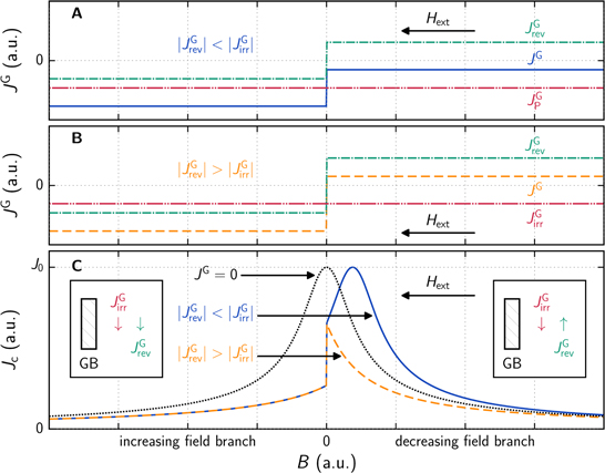
Figure 2. Simplified dependence of  ,
,  , and
, and  on an external field which is ramped from positive to negative values (A and B), and the impact on
  predicted by (5) (C).
Download figure:
Standard image High-resolution imageAccording to the model, the shift of the inter-grain magnetization peak near zero field is determined by the values of  and
and  . This is seen in figure 2C, where
  is calculated from (5) from which we know that the maximum current density J0 occurs at k = 0. The dotted curve shows the case
  , where the peak is located at B = 0. If
  (see figure 2A), the maximum of
  occurs in the decreasing field branch, because
  is negative in the decreasing field branch and thus
  subtracts from
  in (2). The larger
  is, compared to
  , the further the peak (i.e. k = 0) is shifted to higher fields of the decreasing field branch. If the absolute values of
  and
and  are exchanged (see figure 2B), the maximum of
  is located at B = 0 but is smaller than J0 because
  is positive in the decreasing field branch and therefore:
  . The behavior is unchanged in the increasing field branch because
  and
and  flow in the same direction, thus the value of
  is the same although the values of
  and
and  are exchanged.
The return field effect [15, 20] and the effect just described always occur together because both originate from  . Nonetheless, for small grains with a moderate aspect ratio, the latter is far more important.
3. Samples and experiments
We investigated three optimally K-doped and three optimally Co-doped polycrystalline Ba-122 bulk samples. The K-doped samples were synthesized using a mechano-chemical reaction path described in [27]. The grain size was controlled by applying different temperatures during the final heat treatment. The samples were sintered for 10 hours in a hot isostatic press at  ,
,  , and
, and  , where lower temperatures result in a smaller grain size.
The Co-doped Ba-122 polycrystalline bulk samples were synthesized using different starting powders and processing techniques [28]. For the large- and medium-grained samples, the starting materials were Ba, FeAs, and CoAs, while elemental powders were used for the small-grained sample. The powder of the large-grained sample was mixed and ground in an agate mortar and the other two samples were mixed by high-energy ball-milling. All samples were heat treated for 48 hours at  for the large- and medium-grained sample and at
  for the small-grained sample.
The magnetization of all samples was measured in a  SQUID magnetometer and a
  vibrating sample magnetometer. The field profiles of the samples were recorded using a SHPM set-up with a spatial resolution of approximately
  , and a scan range of
  , which is located in an
  cryostat with an operable temperature range of approximately 3−300 K. The size of the active area of the Hall-probes is
  .
.
The size of the grains is statistically distributed, which is described by the distribution density function  (4). The value s0 defines the grain size where the distribution density function has a maximum, which is approximately 0.1, 1, and
  for the different K- and Co-doped samples. These characteristic grain radii are referred to as small, medium, and large. As an example, figure 3 shows the grain radii distribution density and its fit for the medium-grained K-doped sample, which was evaluated from polarized light images of the sample surface by choosing multiple lines of the image and measuring the distance from one GB to another. The grain size distribution of the large-grained sample was evaluated in the same way while s0 of the small-grained sample was roughly estimated from transmission electron microscopy images utilizing the intercept technique [13].

Figure 3. Grain size distribution density of the K-doped sample with medium-sized grains and the fit with equation (4), where m = 3. The bars represent the normalized number of grains with a radius in the interval  , which is given by the width of the bars.
Download figure:
Standard image High-resolution image4. Field profile evaluation
The inter- ( ) and intra-grain current density (
 ) are extracted from SHPM data, i.e. the field profiles above the samples. We evaluate
  by fitting an analytical function derived in [29] to the global field profile, where the spatially constant parameter
  is the only free parameter. Figure 4A shows an example for a field profile generated by
  .
.  crosses the GBs as illustrated in figure 4C, leading to the global field profile shown in figure 4A.

Figure 4. Illustration of global field profiles generated by inter- and intra-grain currents (A and B) and a sketch of the current flow in the sample (C and D). The rectangles in C and D represent the grains. The arrows in C and D are illustrative, i.e. their lengths are not proportional to the actual values.
Download figure:
Standard image High-resolution imageThe intra-grain current density  is confined to the individual grains as indicated in figure 4D by the small arrows. If the distance between the Hall-probe and sample surface is larger than the dimensions of the grains, the fields, which are generated by the intra-grain current densities of neighboring grains, cancel each other in a first order approximation (hatched area), except for a narrow region at the sample edge. Thus, the intra-granular field profile can be approximated by a field profile resulting from a current density,
  , flowing in a thin surface layer of thickness s0 (large dashed arrows). The resulting field profile for this case is plotted in figure 4B. To fit the field profile originating from
  we again utilize the equation from reference [29]. With this technique we are able to evaluate
  from SHPM data quantitatively.
Figure 5 shows examples of field profiles obtained from the medium-grained K-doped sample and fits of the aforementioned analytical function. The field profiles were recorded along a field run from 3 to  . First the profile was measured in the decreasing field branch at
  and then in the increasing field branch at
  .
.  can be identified as the slopes at the sample edges in SHPM measurements, while
  is proportional to the slopes in the remaining sample space, as indicated in figure 5A.
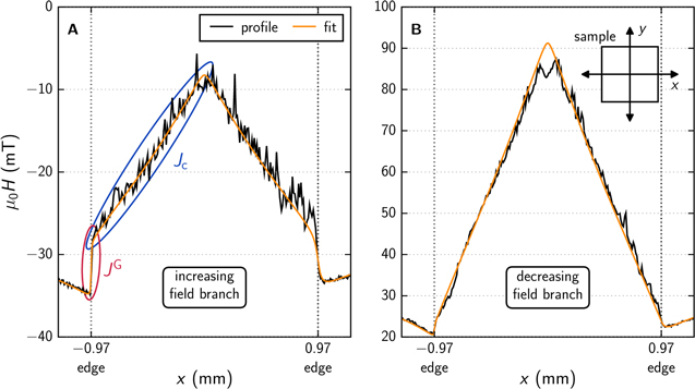
Figure 5. Examples of fits to the field profiles of the medium-grained K-doped sample. The dotted vertical lines indicate the sample edges. The scans were performed across the sample center (y = 0) as defined by the inset in the upper right corner of panel B. Note the much larger trapped field in the decreasing field branch.
Download figure:
Standard image High-resolution imageIn order to make the SHPM results comparable to the magnetometry data, the obtained values for  and
and  are converted to a magnetization M using the standard formula for cubic samples [30] (compare to section 5.2, e.g. figure 8).
5. Results and discussion
5.1. Qualitative discussion
Figure 6A shows the hysteresis of the transport current density ( ) of a K-doped Ba-122 wire. The radius of the grains is approximately
  . This hysteresis corresponds to an asymmetry in the magnetization M of a bulk sample with a similar grain size, which is highlighted in figure 6B by the shaded areas. The asymmetry is given by the difference between the decreasing field branch (
 ramped to smaller values) and the increasing field branch (
 ramped to larger values) after mirroring the latter about the reversible magnetization
  , as defined in [31] with
  and
and  . The comparison between
  in figure 6A and the
  evaluated from magnetization measurements shows good agreement [13].
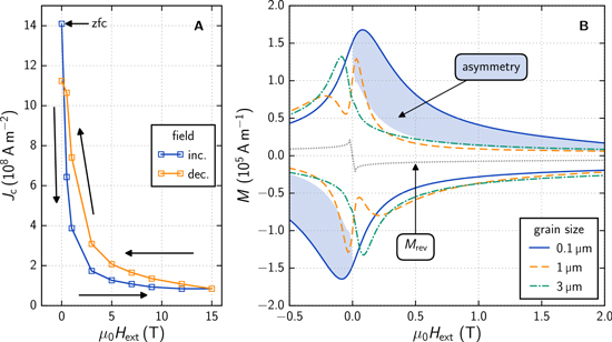
Figure 6. Hysteresis of the critical current density between the increasing and decreasing field branches of a K-doped Ba-122 wire with a modal grain radius (s0) of approximately  measured by transport current (panel A) at
  . Magnetization loops of polycrystals with different grain sizes measured in a vibrating sample magnetometer (panel B) at
  .
.
Download figure:
Standard image High-resolution imageAnother distinct feature is the different behavior of the samples in figure 6B. The curve of the large-grained sample (dash-dotted curve) is very similar to the magnetization curve of single crystals with the maximum value of M in the increasing field branch and its asymmetry is small. The asymmetry increases with decreasing grain size and another peak near  emerges for a grain radius of
  (dashed line). This peak is located in the decreasing field branch and becomes larger and wider when the grain radius is decreased to
  (solid line), while the peak located in the increasing field branch disappears.
The Co-doped samples exhibit a similar behavior with a smaller magnitude of the magnetization curves. We observe the largest asymmetry in the sample with the smallest grain size, the two peaks in the magnetization curve of the medium-grained sample, and only one peak in the increasing field branch for the large-grained sample. This indicates that the asymmetry effects are governed by the grain size of the individual polycrystals and not by the dopant, therefore we concentrate on the results obtained from the K-doped samples.
Figure 7 displays the field profiles of the K-doped samples measured at various constant external fields along a run from 3 to  . In the small-grained sample (figure 7A), the field profiles in the decreasing field branch are shaped roughly in accordance with Bean's critical state model, i.e. a constant slope of the field profile corresponding to a spatially uniform
  . Hardly any contribution of the intra-grain currents is observed when looking at the sample edges, which indicates that the peak in the decreasing field branch in figure 6B originates from the inter-grain currents. When the field is ramped through zero, the field profile starts to 'collapse' from the sample edges towards the center. The difference in the magnitude of the slopes at comparable positive and negative fields is striking. For instance, the slope at
  (decreasing field branch) is 3 times larger than at
  (increasing field branch).

Figure 7. SHPM measurements on the K-doped samples along a field run from 3 to  . The spatial extent of the samples is indicated by the vertical dotted lines. The Hall-probe was kept at a constant z-position, and the distance to the sample surface was approximately
  in the scans of the small-grained sample, and approximately
  for the medium-grained sample. In the case of the large-grained sample the sample surface was tilted relative to the scanning plane, i.e. at the left edge
  and at the right edge
  .
.
Download figure:
Standard image High-resolution imageNo Bean-like field profile is observed for the large-grained sample (figure 7C). Instead, a rather flat field distribution across the sample is present, except for a large field gradient at the sample edges. This is characteristic of a field profile dominated by the contribution of the individual grains and thus the peak in the increasing field branch in figure 6B is caused by the intra-granular current of the grains.
The measured field profiles of the sample with the medium-sized grains show an intermediate behavior between the large- and small-grained samples (figure 7B). When the field is ramped from the maximum applied field to zero, an inter-granular field profile builds up, while hardly any contribution of the intra-grain currents is observed. When the field passes through zero, the sample behaves like the small-grained sample, i.e. the slope of the inter-granular field profile becomes smaller. Simultaneously, the intra-grain currents emerge and start to dominate, leading to a flat field distribution across the sample. The hysteresis of  is clearly visible when a field profile of the increasing field branch is compared to one recorded in the decreasing field branch at the same
  . In the decreasing field branch the profiles exhibit a much steeper slope, whereas
  is noticeably larger in the increasing field branch.
The SHPM data in figure 7 reveal that the magnetization peak in the decreasing field branch in figure 6B originates from the inter-granular current density  , and the peak in the increasing field branch originates from the intra-granular current density
  . Accordingly, the peak of the small-grained sample is determined by
  . The position of this peak on the field axis is generally explained in the context of the return field of the grains,
  , which results from
  . Following [20], the peak occurs when the local magnetic induction at the GBs is zero, i.e. when
  , and therefore
  coincides with the field at which the peak is found:
  . The value of
  necessary to generate this field is:
  , for a moderate aspect ratio of the grains (which is true for the investigated small-grained sample). If we compare this value to the maximum current density found in K-doped Ba-122 single crystals[21]:
  , the return field on its own appears to be a highly questionable explanation for the observed behavior.
Clear evidence that  alone cannot be responsible for the
  -hysteresis is observable in figure 7A. Simply put, the return field has to be of the order of the trapped field inside the grains which corresponds to the height of the field step at the sample edges (compare figures 4B and 5A). Since the step height barely depends on the actual geometry of the intra-granular current flow, this argument includes scenarios where the magnetic grain size differs from the crystallographic grain size (s0), i.e. the formation of grain-clusters, characterized by a number of connected grains with low-angle GBs that do not hinder the current transport from one grain to another and therefore behave like a single grain. However, such a field step is not present in the SHPM measurements in figure 7A. Consequently, another effect has to contribute to the hysteresis of
  .
.
The model presented in this paper can account for this behavior using much smaller values of  . As discussed in section 2, the peak position of
  is determined by
  and
and  (
( ). To shift the peak of the small-grained sample to the experimentally determined
  ,
,  has to attain a value of approximately
  in the decreasing field branch—a much more realistic current density. Our SHPM data directly confirm the predictions of the presented model. We will show this below for the medium-grained sample, which allows the simultaneous detection of inter- and intra-grain currents.
5.2. Quantitative evaluation
The magnetizations predicted from the SHPM measurements on the medium-grained sample, i.e.  stemming from the inter-grain current density (
 ), and
  stemming from the intra-grain current density (
 ), are shown in figure 8. The values are extracted from the data shown in figure 7B as described in section 4. The sum of the two contributions agrees well with the SQUID data, which supports the reliability of our evaluation procedure. The equally evaluated data of the small- and the large-grained samples (figure 7A and B) also show good agreement between the magnetometry and SHPM measurements.
At  , the applied field where the maximum magnetization is observed, the slope of the global field profile corresponds to a
  of approximately
  . The value of
  at the intra-grain peak position (
 ) is approximately
  .
.
The  values, obtained from the SHPM data, together with equation (5) are used to calculate a value of
  and consequently
  , the magnetization corresponding to the predicted
  . The grain radius distribution parameters m = 3 and
  are evaluated from images of the sample surface (see section 3). The self-field of the sample is taken into account by substituting
  in (2), where
  is the difference between the maximum and minimum field values of the (measured) field profile. The thickness of the GBs, d, the penetration depth λ, and the maximum current density, J0, are the fitted parameters. The obtained values of
  are plotted in figure 8 for comparison with
  .
.
Figure 8 shows the advantage of large-area SHPM scans. The sum of  and
and  clearly reproduced the unconventional double-peak in the magnetization curve
  , and
, and  closely follows
  . The fitted value of
  corresponds to the maximum inter-grain current density extracted from the field profiles in figure 7B (
 ). The penetration depth
  is comparable to the results obtained in [32], where the authors found a value of
  at
at  . In [33] the authors investigated identically synthesized samples by atom-probe tomography. Their data show that the length scale of the composition variation of Ba, K, Fe, As, and O across the GBs is about 5–
 . This length is comparable to the fitted total thickness of the GBs:
  .
.
6. Implications
We discussed the hysteresis of  in dependence of
  in figure 2. In the increasing field branch
  and
and  flow in the same direction and
  is large while
  is small. According to the presented model,
  in the increasing field branch should decrease further if
  becomes larger. To validate this prediction, a bulk sample with an approximate grain radius of
  was exposed to fast neutron irradiation. This procedure induces defects in the crystallographic structure of the grains which are capable of pinning flux-lines, thus increasing
  [34]. Magnetization measurements performed after neutron irradiation confirm the decrease of
  in the increasing field branch. This implies that a smaller value of
  would increase
  , i.e. the pinning in polycrystalline HTS with large-angle GBs should be minimized.
The impact of the modal grain radius, s0, on the inter-grain critical current density,  , is most interesting in view of the production of technical superconductors. In contrast to k, s0 is independent of the field and allows a more precise interpretation. Figure 9 visualizes the dependence of
  of a Josephson junction network with different s0 in the decreasing (A) and increasing (B) field branches. A small s0 in equation (5) entails a diminished field dependence of
  . The dashed arrows in the graphs highlight the corresponding increase of
  .
.

Figure 8. Magnetization values calculated from SHPM measurements on the medium-grained K-doped sample (figure 7B). The inter- ( ) and intra-grain contributions (
 ) are plotted separately.
  denotes the fit of (5) to
  , and
, and  is the magnetization measured in a SQUID magnetometer (inter- and intra-grain contributions). Errors correspond to one standard deviation of the respective fit parameter,
  or
or  .
.
Download figure:
Standard image High-resolution image
Figure 9. Dependence of  on the modal grain radius s0 in the decreasing (A) and increasing (B) field branches. The value of
  is arbitrary.
Download figure:
Standard image High-resolution image
In the framework of the presented model the most advantageous grain size of a weak-linked superconductor is as small as possible. For the examined iron-based superconductors the grain size can be changed by milling the starting materials and by varying the heat treatment of the bulks. The model neglects the influence of the grain size on other superconducting properties, such as the transition temperature, the upper critical field, or the anisotropy. In reality the optimal/minimal grain size will be determined by the deterioration of the superconducting properties of the grains.
Neglecting this deterioration, a magnetic induction  can be extracted from figure 9B up to which a wire with a certain grain size can be used in typical applications. The value of
  is defined by the point where
  drops below a minimum value
  , which is determined by the required critical current density of a certain application (see figure 9B).
  can be derived from (5). For typical values of λ (
 ), d (
 ), and
  (
( ) the field dependence of k is mainly determined by the term
  for
for  , which is true for high-field applications. In this case
  is smaller than 1 and (5) can be expanded into a Taylor series at
  , yielding the first order approximation:
The value  typically lies in the range of 108–
 , depending on the filling factor of the wire and the envisioned application. Equation (6) indicates that
  , which defines the operable field range of a wire, can be increased by one order of magnitude by reducing the grain size by one order of magnitude.
7. Conclusions
We presented a model describing the history dependence of  found in polycrystalline HTSs. The irreversible currents in the grains reduce
  in the increasing field branch, while they enhance it in the decreasing field branch. We investigated K- and Co-doped Ba-122 polycrystals of three different grain sizes via magnetization and SHPM measurements. With SHPM, both the inter- and intra-granular current density are accessible, which makes SHPM measurements superior to magnetization and transport measurements in order to understand the current flow in granular materials. The model is able to describe the obtained inter-granular current densities based on the intra-granular current densities both qualitatively and quantitatively. It allows the estimation of the field range in which a wire can be operated from the size of the grains inside the wire. This field range increases significantly as the grain size is reduced, a feature which is confirmed experimentally. Our results show that the grain size is a key parameter for increasing the maximum operable field range of polycrystalline HTS materials that are governed by Josephson tunneling. In its essence the model is independent of the material, and therefore our findings are also relevant to other HTS materials.
Acknowledgments
We are grateful to F Sauerzopf and H W Weber from TU Wien for helpful discussions and wish to thank W L Starch and R B Richardson for technical contributions at the National High Magnetic Field Laboratory. The authors gratefully acknowledge Y Hayashi, J Shimoyama, and K Kishio from The University of Tokyo for experimental assistance and discussions. This work was supported by the Austrian Science Fund (FWF): P22837-N20 and by the European-Japanese collaborative project SUPER-IRON (No. 283204) and was partially supported by JST PRESTO and by Grant-in-Aid for Scientific Research from the JSPS (Grant No. 15H05519). The work at the National High Magnetic Field Laboratory was supported by NSF (No. DMR-1306785) to E E Hellstrom, and the facilities of the NHMFL are supported by the State of Florida and by the NSF through a facility grant (No. DMR-1157490).