

Abstract
In experimental fluid mechanics, measuring spatially and temporally resolved wall shear-stress (WSS) has proved a challenging problem. The micro-pillar shear-stress sensor (MPS3) has been developed with the goal of filling this gap in measurement techniques. The MPS3 comprises an array of flexible micro-pillars flush mounted on the wall of a wall-bounded flow field. The deflection of these micro-pillars in the presence of a shear field is a direct measure of the WSS. This paper presents the MPS3 development work carried out by RWTH Aachen University and Purdue University. The sensor concept, static and dynamic characterization and data reduction issues are discussed. Also presented are demonstrative experiments where the MPS3 was used to measure the WSS in both water and air. The salient features of the measurement technique, sensor development issues, current capabilities and areas for improvement are highlighted.
Export citation and abstract BibTeX RIS
1. Introduction
In fluid mechanics, one of the most common flow fields encountered is the flow of a fluid over solid boundaries. This is a complex flow field where momentum and energy are transferred between the wall and the flow. One of the engineering measures of this transfer is the drag experienced by the wall. The skin friction or viscous contribution to this drag is calculated by integrating the shear-stress τw, or skin friction over the entire wall. This skin friction drag has significant physical and financial implications. For example about 40–50% of the drag on a long-haul aircraft is attributed to skin friction drag [1]. Similarly, a significant portion of the power used to pump oil across continents is used to overcome skin friction drag. Also, health conditions, such as atherosclerosis, have been related to the magnitude of the shear-stress within biological systems [2]. Hence, the wall shear-stress (WSS) has compelling economical importance in a wide variety of flow fields over different flow regimes and disciplines.
In wall-bounded turbulent flows this momentum transfer occurs within the boundary layer adjacent to the wall. Embedded within the turbulent boundary layer is a rich cascade of flow structures which form the transfer mechanism of this momentum. The instantaneous WSS is a footprint or signature of these individual unsteady flow structures [3–5]. The growth of the field of flow control over the last decade has necessitated an increased understanding of the interaction between the structures within the boundary layer and its footprint on the wall. Recently, Hutchins et al [6] have quantified this interaction by showing that the wall footprint is actively modulated by the large-scale structures in the logarithmic layer. The WSS is thus a key piece of information in further understanding the interaction between the near-wall cycle and the outer layer cycles. Therefore, beyond the financial implication, there is a need for WSS measurements to advance the understanding of wall turbulence, especially with the goal of controlling it.
Excellent reviews of the advances made in the measurement of WSS have been presented by Naughton and Sheplak [7], Plesniak and Peterson [8], Löfdahl and Gad-el-Hak [5], and Haritonidis [9]. Readers are referred to these reviews for information on existing WSS measurement techniques. Most current techniques can provide accurate mean, spatially distributed WSS measurements (oil-film based techniques) or unsteady measurements at a point (hot-film sensors). Sensors enabling the measurement of unsteady WSS mostly measure one-dimensional WSS or the magnitude of the WSS. In turbulence research, however, it is desirable to be able to detect spatially resolved two-dimensional, i.e. span-wise and stream-wise, temporal distribution of WSS. This task has proven historically challenging in experimental fluid mechanics. Naughton and Sheplak [7] aptly concluded their review by stating that 'the development and calibration of a reliable shear-stress sensor that can provide fluctuating shear-stress for flow control applications is particularly desirable'.
The challenges in measuring the unsteady, distributed WSS are many. The level of the WSS, at most Reynolds numbers relevant to engineering flows, is extremely small (≈1 mPa to several Pa). However, in spite of the overall stresses measured being small, the relative magnitude can vary substantially between flow fields. For example, consider flow over a flat plate in air and water. When the stream-wise location, skin friction coefficient and Reynolds numbers are identical, the magnitude of the mean WSS measured in water is several orders of magnitude higher than that in air. Hence, in most circumstances a sensor has to be designed specifically for a given flow field.
Also, the smallest turbulent fluctuations that need to be resolved are about 10–20% of the mean WSS. These fluctuations can occur abruptly and rather violently, which results in sharp spatial and temporal gradients. For example, in a flow field with Reynolds number (based on stream-wise distance and free-stream velocity) of ≈106 the smallest characteristic length scale (Kolmogrov scale) is of the order of a hundred µm. The largest length scales that are present in the flow field are of the order of the size of the boundary layer, which is of the order of tens of cm.
While the lowest frequencies present in the flow field are of the order of 10 Hz, the maximum frequencies present in the flow field are of the order of the Kolomogrov scale, which is of the order of hundreds to thousands of Hz. This variety in scales requires a sensor with large enough bandwidth that can resolve all the scales present within the turbulent boundary layer. This problem becomes exacerbated when the Reynolds number is increased as the scale separation between the largest and the smallest scales becomes more pronounced.
A flexible polymer WSS measurement technique initially presented by Tarasov et al [10, 11] (cited by Fonov et al [12]) and subsequently used by Amili and Soria [13] has shown promise in performing unsteady, distributed WSS measurements. This technique uses a flexible polymer that deforms elastically under the influence of fluid pressure and WSS, whose deformation is measured optically. Thereafter, an inversion is carried out yielding the surface pressure and WSS distribution. Using this technique several measurements of the distributed mean WSS, in which the working fluid was air [12, 14–16] and water [17], have been carried out. Amili and Soria [13] used the flexible polymer WSS measurement technique to present instantaneous snapshots of the fluctuating WSS distribution in a turbulent channel flow. These preliminary results show promise in measuring unsteady, distributed, spatially resolved WSS resolving frequencies up to 120 Hz.
The sensor discussed during the course of this report is inspired by some commonplace visualization of the WSS in the atmospheric turbulent boundary layer—such as the motion of corn heads on a windy day or streaks on the water surface of a lake. Small micro-pillar type appendages have also been observed in biological cilia, in insects, to detect precisely the motion of prey [18]. Horridge describes the localization of prey by non-motile cilia with the aid of small displacements in the surrounding water [19, 20]. It has been shown that the WSS in the cardiovascular system drives the gene expression in endothelial cells and is considered to play a role in its development [2, 21, 22]. Van der Heiden et al [21] postulate that micro-pillar like immotile cilia in chicken embryonic endocardium acts as biological WSS sensors of endothelial cells aiding in changes to the gene expression.
This research work presents the combined, modest progress made by separate research groups at RWTH Aachen University and Purdue University in the development of a WSS sensor inspired by these naturally occurring phenomena. The WSS measurement technique discussed is the micro-pillar shear-stress sensor (MPS3) which was initially presented by Brücker et al [23]. It has been demonstrated that the MPS3 has the ability to measure unsteady, distributed WSS in fluid flows. As part of this report, WSS sensor requirements are presented, followed by descriptions of the current sensor concept. General description of the manufacturing techniques along with recent advances in the manufacturing technique such as the use of aluminum molds and reusable molds are discussed. Static and dynamic characterization of the MPS3 is discussed. A MPS3 with resonance frequency >5 kHz as well as phase characterization of a typical MPS3 are presented for the first time. The recent challenges encountered in the measurement of WSS in air using MPS3, namely the useful frequency range of the MPS3 and data reduction challenges, are discussed. Finally, demonstrative measurements of WSS in flow fields where the working fluid is water and air are presented.
2. Sensor concept
The micro-pillar shear-stress sensor MPS3 is based on cylindrical micro-structures which are positioned on the wall. A schematic of the concept is presented in figure 1. The micro-pillars are exposed to the fluid forces which cause them to bend depending on the prevailing WSS. Hence, the measurement technique belongs to the indirect group of measurement techniques [9], since the WSS is derived from the relation between the detected velocity profile and the local surface friction. Due to its cylindrical geometry, the sensor is equally sensitive to both wall-parallel WSS components and does not suffer from cross-axis sensitivity. Consequently, the micro-pillar deflection can be considered to be representative of the exerted forces, both in magnitude and angular orientation.
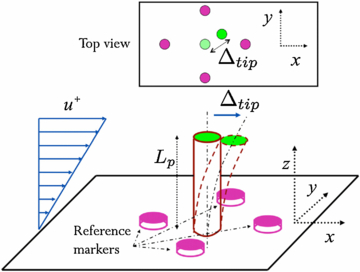
Figure 1. Schematic of the micro-pillar WSS sensor concept [24].
Download figure:
Standard image High-resolution imageEquation (1) shows the relation between the WSS τw and the deflection Δtip of the sensor.
where E is Young's modulus, Lp the length and Dp the diameter of the pillar and τw the local shear-stress. Formula (1) has been derived assuming linear bending theory for a circular beam with plain shear flow exerting on it. The shear forces have been estimated using Oseen's approximation for the drag load per unit length of the cylinder. Note, the deflection Δtip depends on the fourth power of the aspect ratio, i.e., length to diameter ratio Lp/Dp. Since the micro-pillars possess a high aspect ratio of the order of 7 to 15 and are made of an elastomer, they are extremely flexible, which ensures their high sensitivity.
Nevertheless, a static calibration is necessary to correlate the deflection of the micro-pillars with the local WSS. The sensor is placed in a Couette flow where the sensor is exposed to a linear velocity profile. Consequently, the sensor length is limited to the thickness of the viscous sub-layer since the sensor has to be exposed to the same load in the measurement as in the calibration case. Typical calibration curves for different sensor lengths are shown in figure 2. For lower shear rates (Δtip/Lp ⩽ 20%), the deflection Δtip is proportional to the shear rate τw (cf figure 2(a)). At higher shear rates—as shown for the micro-pillar with Lp = 100 µm in figure 2(b)—there is a nonlinear relation between Δtip and τw.

Figure 2. Calibration curves for different pillar geometries (green: Lp = 100 µm, red: 200 µm, blue: 300 µm and black: 400 µm).
Download figure:
Standard image High-resolution imageFor most turbulent flows of low to moderate Reynolds numbers the height of the viscous sub-layer is between 60 and 1000 µm. Thus, this height is a manufacturing constraint. According to formula (1) the sensitivity is dependent on the length of the micro-pillar, as the shear force at the tip of the micro-pillar contributes minimally to its deflection. The micro-pillar deflects predominantly due to the drag force experienced as a result of the flow past its length. The requirement that the sensor lies within the sub-layer ensures that the sensor does not influence the flow, while providing maximum sensitivity. If the height Lp of the micro-pillar is such that it is within the sub-layer, it is generally accepted that any disturbance caused is damped out by the viscous forces [25]. Große et al [26] show using their experiments employing micro particle image velocimetry (µPIV) that the flow is not disturbed by the sensor. The flow field around a micro-pillar lies in the Stokes flow regime as the Reynolds number ReDp based on the local velocity and the pillar tip diameter is well below 1. It ranges from 8.76 × 10⁻³ to 8.76 × 10⁻² [26]. Figure 3 shows the streaklines around the micro-pillar when the Reynolds number based on the micro-pillar diameter is 5.26 × 10⁻⁴. It is seen that the streaklines possess a symmetric curvature and no separation zone in the wake of the structure is identified. The presence of the micro-pillar affects the flow field to about three pillar diameters downstream of the micro-pillar. Thus, a minimum spacing of ≈5Dp between two neighboring micro-pillars is required to minimize interference between micro-pillars.
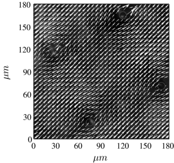
Figure 3. µPIV measurement of the flow around pillars. Local Reynolds number based on pillar diameter 5.26 × 10⁻⁴ [26].
Download figure:
Standard image High-resolution imageThe deflection of the micro-pillars is detected by a highly magnifying optical system which is positioned perpendicular to the surface measured. Additionally, the micro-pillar tips are spotted with a reflective coat, tipped with reflective spheres or marked with fluorescent dye to provide high contrast images. This enables high accuracy tracking by the optical system. The minimal resolvable WSS depends on the optical resolution of the system. The WSS corresponding to about ≈1/10th of a pixel, which is the typical resolution of particle tracking schemes [27], is the nominal minimal resolvable WSS. Adapting the optical resolution to the sensor and flow field, shear-stresses as small as 10 mPa could be successfully measured, although by increasing optical magnification, even smaller ranges are potentially possible.
The use of an optical system to detect the deflection of the micro-pillars reduces the complexity of the measurement system and it allows the simultaneous measurement of the two wall-parallel components of the WSS. Furthermore, using a two-dimensional array of micro-pillars, the measurement of the WSS distribution of a turbulent flow at high spatial resolution is possible. Spatial resolutions as small as 5 l+, where l+ defines a viscous unit, are possible since the MPS3 system does not require further equipment at the wall which would restrict its spatial resolution. However, the setup requires optical access and limits the temporal resolution to the sampling rate of the camera system. Nevertheless, optical access can be provided in the majority of the cases and high-speed camera systems allow sampling at several kHz, which enables the detection of the complete turbulent frequency spectrum. The micro-pillar tip deflection is measured from images of the micro-pillar tip motion obtained using a high-speed camera system using standard particle tracking techniques [27]. Thus, the MPS3 offers the means to measure the instantaneous WSS over an area with the acquisition of a single image.
The micro-pillar protruding into the flow field deflects due to the integration of the near-wall velocity field along its length. As stated, the micro-pillars are submerged within the viscous sub-layer. However, the velocity field in this region is known to have large fluctuations around its mean values and there is currently only a vague idea on the validity of the linearity of the instantaneous velocity distribution. Higher-order moments of the velocity fluctuations for example, i.e., skewness and flatness distribution, indicate a dependence on the wall distance [28–32], indicating the nonlinearity of the instantaneous velocity field. But due to the integration of the viscous forces on the sensor structure along the pillar length, any nonlinearity of the instantaneous velocity gradient within the viscous sub-layer will be damped.
Furthermore, the MPS3 tip deflection does not solely originate from the WSS but is rather the consequence of several contributing effects. Two different kinds of sensitivity-related issues arise. On the one hand, the direct impact of forces other than the viscous drag force, such as forces resulting from local pressure gradients, lateral lift forces resulting from non-uniform flow and influences from external accelerations, to name only a few effects, need to be addressed. On the other hand, changes in the sensor sensitivity itself might have a negative effect on the sensor function. These sensitivity aspects have been elucidated in great detail in [33].
A cylinder [34] placed in a shear flow experiences lift forces perpendicular to the mean velocity direction and to its axis. The integrative effect of this induced lift could add to a deflection of the sensor due to the applying drag forces. However, due to the small lateral dimension of the sensor structure of  (
( being the diameter of the sensor in viscous units), and the lateral velocity gradients the lift-induced deflections of the sensor structure can be considered negligible.
Contribution due to accelerations on the micro-pillar (e.g., vibrations of the experimental setup) should be accounted for especially if very small WSS is to be detected (cf section 5). However, in non-accelerating flow facilities inertial effects can be neglected. While considering changes in the sensor sensitivity, only temperature-related effects have a relevant influence. Chemical and load-related changes of the sensor material and its mechanical properties have negligible effects on the sensor sensitivity [33]. By carefully arranging experimental conditions ensuring constant fluid temperature, temperature effects can be neglected.
3. Manufacturing technique
As described in section 2, the sensitivity of the sensor primarily depends on the aspect ratio and Young's modulus of the sensor material (equation (1)). Consequently, the primary goal in the manufacturing of the micro-sensors is to manufacture micro-pillars with an aspect ratio of at least 7 while the length of the micro-pillars should not exceed Lp = 80–1000 µm. Achieving such a high aspect ratio is a major manufacturing challenge making many traditional micro-manufacturing techniques such as lithography not suitable. Furthermore, large sensor fields are required to measure the two-dimensional WSS distribution while simultaneously maintaining high accuracy of the sensor geometry. The production of filigree structures by casting the sensor from a master mold was found to be the most suitable approach to meet these requirements with high reproducibility.
3.1. Wax mold fabrication technique
Wax molds allow the fabrication of micro-pillars in a lost-mold process. While manufacturing high aspect ratio structures the wax mold can be washed off instead of peeling the sensor off the mold. This has the advantage of reducing the risk of tearing off the micro-pillars. On the other hand, the casting mold is fabricated economically.
Two different techniques were used by the research groups at RWTH Aachen University and Purdue University to perforate the wax. At Purdue University holes were micro-drilled into wax using a tool manufactured by an electric discharge machine. The elastomer is then cast into the wax molds and allowed to cure. The wax mold is then removed and the micro-pillar tips marked if desired. Further details of the manufacturing process are discussed in Gnanamanickam and Sullivan [24]. Figure 4(a) shows a micro-pillar fabricated using this technique.
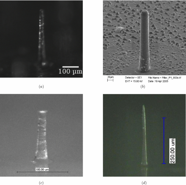
Figure 4. Different micro-pillars fabricated. Sensors cast in (a) wax, using an electric discharge machine, (b) in a laser perforated wax-sheet (Lp = 200 µm) [33], (c) cast in a metal sheet (Lp = 100 µm), and (d) in a polycarbonate casting mold (Lp = 300 µm) [37].
Download figure:
Standard image High-resolution imageThe wax can also be perforated by locally sublimating the wax using laser irradiation [23] as done at RWTH Aachen University. A pulsed excimer laser is used to micro-drill into machinable wax, which is chosen because of its small grain size resulting in good surface quality of the sensors. The diameter of the pillar can be varied depending on the aperture of the laser. In addition, the number of laser pulses determines the depth of the holes and thus the length of the micro-pillar Lp, if blind holes are drilled. In the case of through holes, the thickness of the wax foil sets the length of the micro-pillars. Milling and polishing the wax before the perforation manufacturing step ensures an evenness of the order of 5 µm and thus of the sensor length. But only minimal wax-foil thicknesses of 0.3 mm are feasible. Apart from this limitation, both techniques proved similarly preferable if drilling and curing were carefully performed. A problem where silicon was pouring out of trough-holes forming umbrella-shaped artifacts at the sensor tops could be avoided when properly placing the wax mask, e.g. on a glass surface and locally melting it on it prior to laser drilling.
In general, aspect ratios of the order of 15 can be achieved. Figure 4(b) shows a micro-pillar cast in a through hole. The curvature at the pillar root is due to local surface melting during the ablation process. Its effect on the sensitivity of the sensor is accounted for by the calibration.
3.2. Reusable molds
Not only dissolvable casting molds but also laser perforated metal sheets and polycarbonate substrates were investigated at RWTH Aachen University [35]. Unlike the former manufacturing methods, no a priori treatment is necessary and the mold can be reused nearly infinitely. Figure 4(c) shows a micro-pillar cast in a metal sheet with through holes. The sensor has a length of Lp = 100 µm and an aspect ratio of 7. Since the holes are drilled using laser ablation, the diameter is also adjustable by the aperture of the optical system. The length is determined by the thickness of the high precision metal foils and can be guaranteed within ±4 µm. Higher aspect ratios of about 20 have also been achieved at greater sensor lengths.
Using polycarbonate as mold material enables the manufacture of micro-pillars with comparable high aspect ratios while allowing a further reduction of the sensor length [36]. This makes measurements at higher Reynolds numbers possible. Pillars with a length in the range of Lp = 100 µm have been successfully cast. Figure 4(d) shows a micro-pillar cast in a polycarbonate mold at an aspect ratio of 15. Note the high surface quality of the sensor.
3.3. Cast
In a subsequent step, the elastomer is cast into the mold, degassed and cured under vacuum. Various silicone rubbers have been used depending on the wax type [24] since the combination of silicone and wax strongly influences the quality of the curing. The most appropriate elastomers for the manufacture of micro-pillars are Dow Corning Sylgard 184, Momentive RTV615 and Smooth-On Inc. Solaris which are polydimethylsiloxanes (PDMS). PDMS has a favorably low Young's modulus which improves the sensitivity of the micro-pillars. The sensor is cured for at least 24 h either at room temperature, if cast in wax, or at temperatures of T = 40–180 °C, if a reusable casting mold is used. Subsequently, the sensor is peeled off from the mold using an ultrasonic bath with isopropyl alcohol. The vibrations allow for the detachment of the silicone sensor from the master mold. Though peeling off from a reusable mold is comparable to the wax mold process, using metal sheets can be advantageous because tools like microtome blades can be used for facilitating the peel-off process. However, great care has to be applied. The peeling-off is mainly done by the vibrations and the solvent rather than by any exerted force. However, wax molds for sensors at higher aspect ratios have to be washed off [24, 33] to obtain the sensor.
4. Dynamic calibration
4.1. Mechanical properties
The smallest scales in turbulent flows reduce at higher Reynolds numbers. Especially in air flows, the highest turbulent frequencies can reach several kHz. Therefore, the dynamic behavior, i.e., the frequency response, of the sensor system has to be determined to ensure that these frequencies are within the allowable frequency range of the sensor.
The micro-pillars can be regarded as one-sided clamped cantilevers which experience a linearly increasing load along their length. Furthermore, the micro-pillar can be regarded as a Euler–Bernoulli beam due to the high aspect ratio of a pillar, average deflections below 10% of the structure length Lp and the use of isotropic material PDMS [37–39]. Therefore, the micro-pillars possess a low-pass behavior with a damping coefficient depending on the surrounding fluid. In flows of higher viscosity, e.g., water, the system is overdamped. In air, the system possesses a strong resonance behavior. The dynamic behavior of a micro-pillar can be described by equation (2) where EI denotes the stiffness, w is the lateral displacement at a distinct height y and at a time t.  and
and  are the reduced mass and the reduced damping coefficient of the system, both depending on the local Strouhal number Sr and including the added mass [38, 39].
Große et al [39] assumed Stokes flow around the micro-structure (cf figure 3). That is, they accounted for a frequency-dependent added mass  term. The left-hand side of equation (2) represents the reaction of the sensor to the excitation F(y, t).
However, geometric or mechanical deviations of the micro-pillar dimensions cannot be ruled out during manufacture, thus requiring a dynamic calibration. Therefore, it is necessary to study the characteristic solution of equation (2). Two dynamic calibration techniques were developed to characterize the sensor since Stokes layer excitation [38] is not suitable. Accounting for the various velocity profiles acting on a micro-pillar in an oscillating flow requires an exact analytical determination of the static pillar response to each of the different load cases occurring during a dynamic calibration. This is not feasible, yet. In contrast, Große et al [39] and Nottebrock et al [37] used calibration techniques measuring the impulse response of the system or the frequency response using magnetic excitation of the sensor.
The dynamic calibration by magnetically exciting the sensor structure is described in detail by Große et al [39] with only a brief description presented here. The MPS3 itself is not magnetic, hence a permanent magnet is attached to the pillar tip in addition to the reflective hollow sphere. An electromagnetic coil with a ferrite core is used to harmonically excite the pillars. The coil is sliced and the micro-pillar sensor is installed in the homogeneous magnetic field in the gap thus formed. The response of the pillar to the excitation is recorded at sufficient temporal resolution by a high magnification optical system to ensure a high signal-to-noise ratio. The input function, which is necessary to determine the pillar behavior, is determined by measuring the magnetic field strength simultaneously with the pillar reaction [37].
Figure 5 shows the frequency response of a micro-pillar with Lp = 300 µm and Dp = 20 µm in air. The measured micro-pillar gain fits an analytic second-order model very well. For frequencies beyond the resonance, the gain decreases at a slope of −20 dB, which is characteristic of a second-order low-pass filter. Furthermore, the phase shift is −90° at the resonance frequency f0 identical to the characteristics of a second-order low-pass filter. These results indicate that the micro-pillar possesses a very constant transfer function amplitude at frequencies reasonably below the resonance [39]. The sensor gain can be assumed to be approximately constant at frequencies lower than 0.3–0.4 f0.

Figure 5. Bode diagram for the frequency response of a micro-pillar with Lp = 300 µm: (a) measured gain as a function of excitation frequency (○) compared to the analytical solution of a low-pass filter (dashed line), (b) phase shift for the measured pillar response (○) and the low-pass filter (dashed line) [37].
Download figure:
Standard image High-resolution imageHowever, the magnetic excitation procedure is inconvenient for large sensor arrays. As an alternative to obtaining the eigenfrequency and damping from the frequency response of a micro-pillar, the response of the micro-pillar to an impulse is measured. The frequency response of the system is obtained by a Fourier transformation of its impulse response [40].
The micro-pillar is initially deflected using a small needle that bends the pillar. The needle is abruptly removed and the micro-pillar undergoes damped oscillation as depicted in figure 6. Once the pillar is released, the micro-pillar movement is recorded using a high-speed camera at a recording frequency up to 27 kHz. The sampling frequency ensures a high enough resolution of the temporal response. The magnetic excitation method presented above showed that the micro-pillar dynamic behavior can be approximated well by a linear second-order system. Thus, an impulse response test can be used to determine the eigenfrequency and damping coefficient of the micro-pillar.
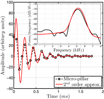
Figure 6. Response of the micro-pillar tip to an impulse. Also shown is the response of a matched second-order dynamic system. The inset shows the power spectrum corresponding to the response of the micro-pillar tip and the second-order dynamic system.
Download figure:
Standard image High-resolution imageResults from a typical experiment are shown in figure 6 (note—the characterization of a different micro-pillar than that presented in figure 5 is shown here). The shown tip displacement is recorded using a high-speed camera (16 000 Hz) in conjunction with a high magnification lens system. Also shown is a second-order system approximating the oscillatory motion of the micro-pillar. A damping coefficient of 0.11 [39] is used in the second-order estimate. The second-order system is seen to match closely the motion of the micro-pillar tip especially past the initially large amplitude motion. Also shown in figure 6 is the power density spectrum corresponding to both the MPS3 and the matched second-order system. The damped resonance frequency of the particular micro-pillar estimated using the eigenfrequency test is ≈5.19 kHz, while the undamped resonance frequency is ≈5.22 kHz. It is noted that there was no added mass used while carrying out this particular eigenfrequency test.
Both methods show very good agreement while estimating the eigenfrequency and the damping coefficient. For the investigated micro-structures, eigenfrequency results from the step response agreed with the results from the magnetic excitation method within an error of a few Hz.
4.2. Aeroelasticity
WSS measurements in turbulent boundary layers in air showed that this model to describe the dynamics of the MPS3 does not agree well with the observed dynamic behavior [37]. The resonance frequency is not at the expected frequency but at lower values. Furthermore, the damping coefficient is higher than the value obtained by dynamic calibration since the peak in the frequency spectrum is not as pronounced. This can be explained by the added mass due to the displaced fluid. The original assumption that the influence of the surrounding fluid is taken into account during the dynamic calibration cannot be confirmed while carrying out measurements in air. The fluid adjacent to the micro-pillar is suspected to be influenced by the movement of the pillar itself such that the micro-pillar can no longer be regarded as only reacting to the surrounding flow field. It becomes an aeroelastic system where the mass and damping of the system in equation (2) depend on the flow conditions. This implies a dependence on the actual deflection of the micro-pillars. As a consequence, the resonance frequency of the micro-pillars is altered and thus the allowable frequency bandwidth. Note, however, that the local Reynolds number is unchanged (cf section 2) such that Stokes flow can still be assumed around the micro-pillars.
This has to be considered during WSS measurements where flow around the micro-pillar has finite velocity in contrast to the dynamic calibration where the fluid around the micro-pillar is at rest. Thus, the assumptions of Brücker et al [38] and Große et al [39] are insufficient. They postulated that the measured values of the eigenfrequency and the damping from the dynamic calibration include the added mass. Consequently, their linearization of the differential equation (equation (2)) has been oversimplified. The results of the turbulent boundary layer experiments emphasize the nonlinearity of the relevant differential equation [37]. Note, however, that while using the unamplified spectrum of the measurement signal, i.e. 30–40% of the resonance frequency, reliable measurements in air can still be performed [37].
5. Background motion
The measurement of WSS has the challenge of measuring very small levels of shear. In large experimental facilities, the ambient facility vibrations add a component of error to the system in the form of relative motion between the optical system and the MPS3. This appears as background vibration while acquiring images. Facility vibrations Δback of the order of several tens of pixels were noticed while the micro-pillar tip deflection Δtip was of the order of a few pixels. Hence, the removal of background vibrations becomes critical in the accurate measurement of not only the WSS magnitude but its frequency content.
The MPS3 concept as presented in figure 1 shows a grid around the micro-pillars. This grid, referred to as reference markers, serves to establish the background motion. These reference markers are also manufactured during the manufacturing process. The micro-pillar tip deflection is then measured with respect to this grid. Alternatively, other surface features are used to accurately establish the background motion. The high-pass filtered (dc removed) background motion magnitude |Δback| from an experiment is shown in figure 7. Also shown is the magnitude of the tip displacement of a single micro-pillar with and without background motion subtraction. The displacements have been axis shifted and only a portion of the entire time record sampled is shown for visualization purposes. The background motion correction was carried out separately in both the wall-parallel directions though only the magnitudes are shown for visualization purposes. The frequency content of the entire time record is shown in figure 8. The removal of the spurious low frequency content of the background motion from the tip displacement Δtip is clearly visible. While carrying out the background motion removal, care is taken to use reference markers or surface features in the vicinity of a given micro-pillar. This is necessary to account for image rotations. In the case of the background motion removal shown in figures 7 and 8, about 25 local reference markers or surface features were tracked. It is noted that the data set presented in figures 7 and 8 is part of the experimental wall jet study presented in section 6.2 below, where the background motion was considerably smaller than that which is noticed in larger facilities.

Figure 7. High-pass filtered magnitude of the background motion along with tip displacement of a single micro-pillar with and without background subtraction. For visualization purposes, only a short period of the entire temporal record is shown and the three different records have been axis shifted with respect to the ordinate.
Download figure:
Standard image High-resolution image
Figure 8. Frequency content of high-pass filtered magnitude of the background motion along with that of the tip displacement of a single micro-pillar with and without background subtraction.
Download figure:
Standard image High-resolution image6. Results
The application of the MPS3 to capture the WSS has been demonstrated in several publications [23, 26, 33, 35, 37, 38, 41–43]. Besides the two flow cases which will be presented in the following sections, experiments in a pipe flow [44, 45] and in a flat plate turbulent boundary layer [37, 43] have been carried out, proving the capabilities of the sensor in accurately measuring the WSS. In the present report, demonstrative results of the WSS measurements in a duct flow (section 6.1) and in a wall jet (section 6.2) are presented.
6.1. Visualization of turbulent structures in a duct flow
6.1.1. Experimental setup
Measurements in a turbulent duct flow have been performed to visualize turbulent structures [41, 42]. The determination of the spatially and temporally varying WSS distributions is of vital importance in turbulence research, since it offers a detailed insight into the dynamic turbulent processes in the vicinity of the wall [35]. A duct flow facility with a square cross section and a hydraulic diameter of H = 42 mm was used (figure 9(a)) to study spatially and temporally varying WSS. The fluid used was deionized water at 20 ± 0.1 °C. The Reynolds number ReH based on the bulk velocity Ub and the duct height H was ReH = 15 000 where the velocity has been calculated from the volume flux, which can be estimated with an accuracy of 0.3%. The resulting Reynolds number based on the friction velocity was Reτ = 900. The friction velocity was determined from the pressure gradient in the measurement section.
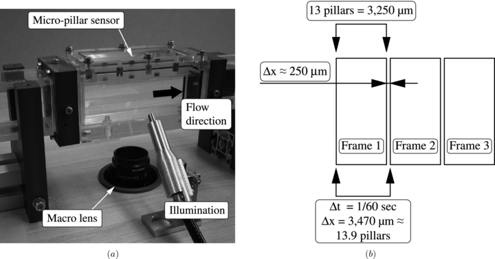
Figure 9. (a) Experimental setup for the measurement of the WSS distribution in turbulent duct flow. (b) Schematic of the sequential recombination of frames in the present study [41].
Download figure:
Standard image High-resolution imageA tripping device with a contraction ratio of 0.85 was used to trigger turbulence. It has a rectangular cross section similar to the duct. The measurement section was located 50 H downstream of the tripping device such that the flow can be considered to be fully developed [46]. However, a secondary flow field evolves in the case of turbulent duct flow resulting in a three-dimensional flow field. Studies of the flow field using particle image velocimetry (PIV) showed that the flow nearly resembles fully developed two-dimensional channel flow in the measurement section [41]. The results from PIV were in good agreement with the findings of a fully developed two-dimensional channel flow at comparable Reynolds numbers [47].
Two different sensor arrays were used to carry out WSS measurements. To visualize the large-scale turbulent structures, an array of 17 × 25 micro-pillars in the stream-wise and span-wise direction, respectively, were used. These micro-pillars had a sensor length of Lp ≈ 160 µm [41]. Thus, the sensor length in wall units was 3.4  and hence the sensor remained fully immersed within the viscous sub-layer. The lateral spacing between the micro-pillars was 250 µm which corresponds to about 5.3 viscous units. The camera was operated at fs = 60 Hz and at full frame. Although the recording frequency was not high enough to detect the highest frequency content, which was estimated to be approximately 250 Hz, the large-scale structures could be well resolved. The total recording period was 8.5 s. During this time span a particle with bulk velocity Ub travels a distance of 75 H. Thus, the data do not allow a complete investigation of the characteristics of turbulent WSS due to the insufficient recording time span [41]. The results presented here rather demonstrate the general ability of the MPS3 technique to detect the two-dimensional WSS distribution in turbulent flows.
Therefore, a sensor with 12 micro-pillars placed along the span-wise direction was used to detect higher frequencies in the flow [42]. However, the sensor length was slightly higher but well within the viscous sub-layer. The lateral spacing was 0.5 mm (10.2 l+) resulting in a field of view of ≈120 l+. The sampling frequency was fs = 1000 Hz, which was sufficient to capture the entire frequency spectrum of the flow. The recording time trec corresponded to about 2250 characteristic bulk time scales T+ = trec/(H/Ub).
Furthermore, Taylor's hypothesis of frozen turbulence was applied to capture the stream-wise extent of the turbulent structures. The convection velocity uc of the second sensor was determined from the temporal two-point correlation of the WSS in the stream-wise direction with the sensor aligned in that direction. For the measurements with the two-dimensional array, a constant convection velocity uc = 10 uτ was used [48]. At a sampling frequency fs = 60 Hz, the structures convect l = uc/fs = 3.5 mm in one time step, which coincides with the spatial distance between 14 micro-pillars (figure 9(b)). Hence, the measurements from 14 pillars in the stream-wise direction were evaluated.
6.1.2. Duct flow results
First, the results of the two-dimensional sensor array are presented. The measured WSS fluctuations were  and
and  , which is in good agreement with the literature [32, 49, 47]. Note,
  is the mean WSS. Alfredsson et al [32] state a WSS intensity of 0.4 from their hot-wire experiments and conclude that lower values are due to inadequate sensor length. However, direct numerical simulations of Hu et al [50] or experiments of Keirsbulck et al [51] show a dependence on Reτ. Nevertheless,
  can be confirmed for the studied Reynolds number. Figure 10 shows the probability density function (PDF) of the WSS fluctuations in both the wall-parallel directions. The WSS components are normalized by the corresponding WSS intensity. These results show good agreement with the experimental data of Miyagi et al [52] and Obi et al [53]. Note their experiments were conducted at Recl = 17 600 and Recl = 6600, respectively, where the Reynolds number Recl was calculated based on the centerline velocity. However, the PDF of the normalized WSS fluctuations is reported to be independent of the Reynolds number [41]. The skewness Sτ, x = 0.95 and Sτ, z = 0.07 as well as the flatness Fτ, x = 4.47 and Fτ, z = 5.46 are in good agreement with the literature [32]. The skewness factor in the span-wise direction indicates the symmetry of the flow.
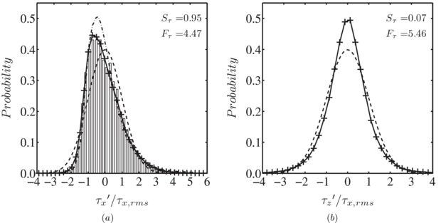
Figure 10. PDF of the (a) stream-wise and (b) span-wise WSS (-+-: present experiments, -·-: Miyagi et al [52] at Recl = 17 600; bars: Obi et al [53] at Recl = 6600, - -: Gaussian distribution) [41].
Download figure:
Standard image High-resolution imageFigure 11 shows a snapshot of the instantaneous WSS distribution of the stream-wise component  obtained applying Taylor's hypothesis. The field shown has dimensions of 2500 × 125 l+. Figure 11 clearly shows that regions of lower and higher WSS coexist and the low-shear regions are locally interrupted by high-shear regions. The dominance of regions of low shear underlines the positive skewness of the WSS fluctuations' PDF (cf figure 10(a)). The positive skewness is indicative of the inherent nonlinearity of the near-wall cycle. The presence of the wall alters the turbulence, causing large but rare high-shear events.
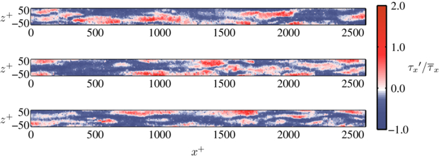
Figure 11. Typical results of an instantaneous WSS distribution in stream-wise direction  using Taylor's hypothesis. Each image possesses a field of view of 2500 × 125 l+ [41].
Download figure:
Standard image High-resolution imageThe sensor detects the footprints of coherent structures present within the boundary layer further away from the wall [41]. These structures have been reported by Kim et al [47] or Moser et al [54], for instance. The streaks seem to meander in the stream-wise direction and their extent near the wall is approximately 40–50z+. This corroborates the findings from the span-wise two-point correlations of the WSS fluctuations in the stream-wise direction ( ) [41]. It corresponds to the mean spacing between neighboring high- and low-shear streaks. Hence, the lateral spacing between two low-shear or two high-shear streaks is about 80–100z+ [41].
Measurements with the line sensor in the span-wise direction underline the general idea of meandering low- and high-shear regions. Furthermore, the MPS3 has been used to identify nearly stream-wise orientated vortices near the wall. These structures go along with wall-normal velocities confirming the three-dimensional character of the near-wall flow [42]. Thus, the MPS3 can be used to detect a footprint of the momentum transfer, which is located in the buffer region of the shear layer. For a more detailed discussion the reader is referred to Große and Schröder [42].
6.2. WSS measurements in a wall jet
The turbulent wall jet is a unique flow field, in that it is a combination of two canonical shear flow fields—a boundary layer and a free jet [55]. A three-dimensional wall jet has the added complexity of a flow field that spreads at a much higher rate in the wall-lateral direction than the wall-normal direction. The wall jet has many engineering applications especially in heating and cooling systems. For example, wall jets are used in the film cooling of jet engine turbine blades and combustion chambers [55]. Launder and Rodi [55] state in their review that wall jets are traditionally used in heating, cooling and ventilating where the 'design has proceeded unfettered by a deep concern about the turbulence structure of the flows in question'. Thus, there is an engineering need to study wall jets. They also provide a framework to study the coupling between the outer and inner structure in three-dimensional flows. It serves as a model three-dimensional flow field with several advantages with regard to experimental instrumentation—it is a three-dimensional flow field with no three-dimensional surfaces. As the free jet and the boundary layer of the wall jet have different inherent scales, they provide the opportunity to modify the wall region independent of the free jet region (far-wall flow) which has interesting implications for flow control [56]. For these reasons the three-dimensional turbulent wall jet was used to evaluate the MPS3. Some demonstrative measurements are presented highlighting the ability of the MPS3 to measure unsteady distributed WSS in a flow field where the working fluid is air.
6.2.1. Experimental setup
A picture of the entire wall jet facility along with labeled salient components is shown in figure 12. Also shown is a schematic of the wall jet exit geometry and the location of the MPS3 with respect to it. Air is regulated into a settling chamber of circular cross section using a needle valve and pressure regulator combination. Prior to flowing into the settling chamber, the air passes through a heat exchanger which brings the air to room temperature. The settling chamber leads into a nozzle with a rectangular cross section, which again ends in the wall jet exit. The nozzle has a honeycomb section within it which acts as a flow straightener. One wall of the nozzle, downstream of the honeycomb section, is a Perspex plate which is also the wall of the wall jet.
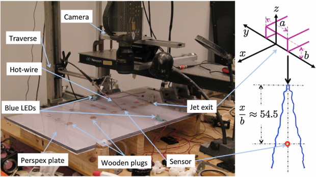
Figure 12. Salient features of the wall jet experimental setup.
Download figure:
Standard image High-resolution imageThe nominal width a and height b of the wall jet exit are 9.55 and 3.5 mm, respectively. The portion of the Perspex plate which comprises the wall jet (portion of the Perspex plate downstream of the nozzle exit) has a length of 662 mm and a width of 512 mm. The overall length of the Perspex plate is 920 mm. The exit of the wall jet was centered to be approximately along the centerline of the Perspex plate. Several holes of diameter 25.4 mm were drilled on the wall portion of the Perspex plate to mount the MPS3. Micro-pillars were cast in an aluminum tube (plug) of outer diameter 25.4 mm and the MPS3 thus formed were flush mounted using the holes on the Perspex plate. During a given experimental run, blank wooden plugs were flush mounted in unused plug holes on the Perspex plate as seen in figure 12.
The stagnation pressure was monitored inside the nozzle, downstream of the honeycomb section, using a pressure transducer. This stagnation pressure was used to set the wall jet exit velocity Vj. The MPS3 was illuminated using blue light-emitting diodes (LED) and the micro-pillar tip motion was tracked using a high-speed camera. The LED were mounted on the Perspex plate, well outside the flow field as seen in figure 12. A three-dimensional traverse and a hot-wire system were used to measure the velocity in the flow field as seen in figure 12. Two types of hot-wires were used to carry out velocity measurements. A straight hot-wire was used to carry out simultaneous hot-wire and WSS measurements. A boundary layer type probe was used to carry out the velocity surveys presented. The hot-wire was calibrated at the wall jet nozzle exit. A single trigger in the form of a TTL pulse from a pulse generator was used to synchronize the camera trigger with the rest of the data acquisition system. A high-speed data acquisition system controlled by a computer was used to sample the pressure transducer and the hot-wire signal along with the TTL pulse of the trigger. The ambient room temperature and pressure were recorded and monitored to get accurate measures of the air coefficient of viscosity and density. The measurements of the wall jet were carried out with a single MPS3 array mounted approximately along the jet centerline as shown in figure 12, at a downstream location of x/b ≈ 54.5. The wall jet exit velocities nominally ranged from 25 to 40 m s−1 in increments of 5 m s−1. The jet exit Reynolds numbers based on the jet exit velocity and the hydraulic diameter ranged from 8.2 × 10³ to 1.3 × 10⁴.
6.2.2. Wall jet characteristics
A boundary layer type probe was used to measure the velocity profile at the rear end of the MPS3. The measured velocity profiles corresponding to varying nominal jet exit velocity, Vj, are shown in figure 13. Figure 13(a) shows the dimensional velocity profile with the inset showing a zoomed-in view of the very near-wall region. As the inset shows, care was taken to make several measurements in the near-wall region to capture the linear portion of the velocity profile. This linear region was used to establish the wall position (z = 0) by extrapolation. This linear velocity profile in the near-wall region also provides an in-situ measure of the mean WSS. Figure 13(b) shows the velocity profile in wall units using the mean WSS calculated. Also shown is a linear profile (u+ = y+) in the near-wall region corresponding to that of a sub-layer. The wall jet clearly has a sub-layer much like a conventional boundary layer which then transitions into the free jet portion of the wall jet without much of a logarithmic region. Estimates of the height of the micro-pillar in terms of wall units range from 5 to 7 depending on the jet exit velocity. The presence of the micro-pillars, the MPS3 mounting and surface imperfections does not appear to break up the viscous linear region, suggesting that the presence of the MPS3 affects the flow minimally. It is noted that there was some span-wise asymmetry especially in the higher order statistics, while carrying out span-wise velocity surveys.
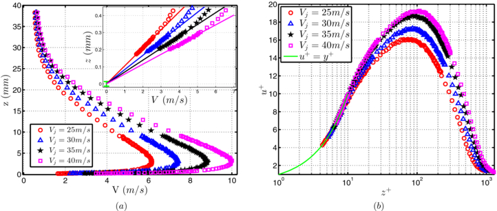
Figure 13. Velocity profiles at the rear of the MPS3 array. (a) The dimensional velocity profiles with the inset showing a detailed view of the near-wall region; (b) the velocity profile non-dimensionalized by wall units.
Download figure:
Standard image High-resolution image6.2.3. Wall jet WSS measurements
The MPS3 is positioned on the wall as shown in figure 12 with a hot-wire at the rear end. The mean WSS vectors, in measured pixel units, when the jet exit velocity is 40 m s−1, overlaid over an actual image of the MPS3 are shown in figure 14. The flow is entering the imaging area from the bottom of the image in the vertical direction. The mean WSS vectors were averaged over three sets of 8900 images—two of the sets were sampled at 3000 Hz and one at 200 Hz. Also seen in figure 14 are the ends of the hot-wire prongs highlighted by green circles. The hot-wire lies within the linear region of the velocity profile shown in figure 13. Figure 14 shows the WSS vectors over a region around the hot-wire being possibly affected by the presence of the hot-wire. Otherwise, over most of the sampled region the WSS is two-dimensional.

Figure 14. Mean WSS vectors over the measurement domain when Vj = 40 m s−1. Also shown are the position of the hot-wire prongs (green circles) and the micro-pillar (cyan circle) whose WSS signal is presented in figure 15.
Download figure:
Standard image High-resolution imageThe hot-wire signal can be directly compared with the WSS signal from the micro-pillar. The fluctuating WSS signal from a single micro-pillar, between the prongs of the hot-wire, as highlighted in cyan in figure 14 is shown in figure 15. Both the stream-wise and span-wise fluctuating components are shown along with the fluctuating raw hot-wire signal. The MPS3 WSS signal and the hot-wire signal have been arbitrarily scaled to aid in comparison. Figure 15 shows that the MPS3 captures almost identically the flow features sampled by the hot-wire. This is evident when comparing the hot-wire signal with the stream-wise WSS fluctuations  . The mean WSS, as measured by the hot-wire survey, is 0.32 Pa and the friction velocity is uτ = 0.52 m s−1. A linear calibration for the MPS3 was assumed across the entire array. The diameter of the micro-pillar is such that the MPS3 measures the WSS averaging over an area of about one viscous length. However, the hot-wire averages over a length of about 30 viscous scales. The spacing between two micro-pillars is about 17 viscous length scales in the stream-wise direction. The camera framing rate is 3000 Hz. The resonance frequency of a single micro-pillar within the array was measured to be ≈5.2 kHz (shown in figure 6). The maximum frequency resolved at this camera frame rate is 1.5 kHz, which is about 35% of the resonance frequency. Hence, the MPS3 measures the WSS at high spatial and temporal resolution with minimal spatial averaging capturing identical flow features to the hot-wire.
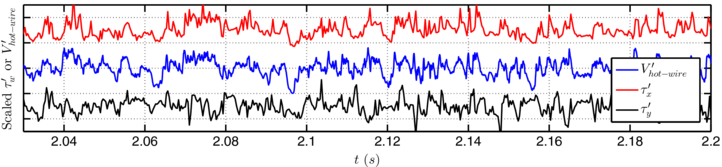
Figure 15. Comparison of micro-pillar tip displacement with the raw hot-wire signal. Note, for visualization purposes the three records have been arbitrarily scaled.
Download figure:
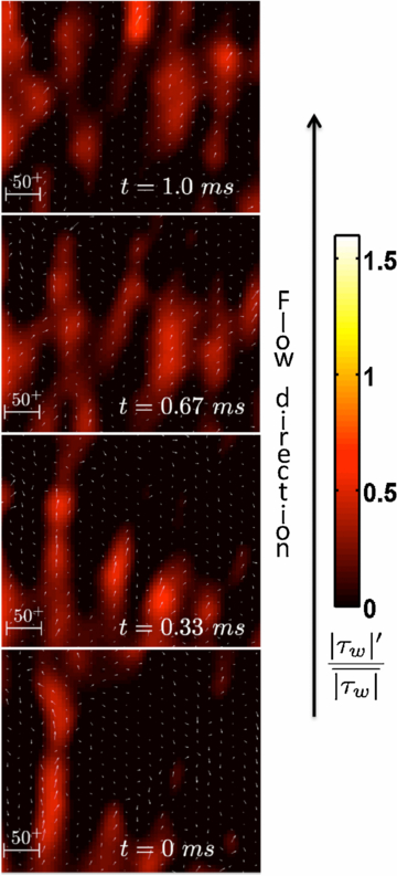
Standard image High-resolution imageUsing an array of micro-pillars allows for the ability to measure the WSS in a distributed manner. The two-dimensional footprint on the wall can be visualized in a spatially and temporally resolved manner. As a demonstration, the evolution of a flow structure is shown in figure 16. The evolution shown in the form of four snapshots forms part of the data set, the results of which are presented in figures 14 and 15. The color contours represent the scaled magnitude of the WSS fluctuations  while the vectors show the instantaneous fluctuating WSS vectors. The four snapshots are separated by 333 µs each. Seen clearly are several streaky structures as they convect across the imaging window. Two of these streaky structures appear to combine and reduce in magnitude as they convect across the imaging area. These streaky structures are high-shear events which are large positive fluctuations in the stream-wise direction. These high-speed streaks are separated by regions of low shear with the fluctuations predominantly being negative.
Figure 16. Time evolution of a flow structure over the measurement window.
Download figure:
Standard image High-resolution image
These preliminary results presented are some of the first distributed, two-dimensional instantaneous WSS measurements that have been carried out in air. The ability of the MPS3 to measure the WSS in an engineering flow field, its comparison with a hot-wire and demonstrative snapshots presented indicate the promise the MPS3 has shown toward carrying out further WSS measurements.
7. Summary and conclusions
The measurement of the temporally and spatially resolved, distributed, wall shear-stress (WSS) in turbulent flows is still a major challenge in experimental fluid mechanics. This report discusses the MPS3 concept to fill this gap in measurement techniques. The sensor is based on flexible micro-pillars which protrude into the viscous sub-layer of a turbulent flow. Since a linear velocity profile can be assumed in the viscous sub-layer, the sensor is calibrated in a Couette flow so that the measured deflection can be correlated with the prevailing WSS. This limits the sensor length to Lp = 100–1000 µm, i.e., the thickness of the viscous sub-layer.
The dimensions of the MPS3 ensure that the sensor does not influence the flow. Visualizations using µPIV confirm that the flow around a micro-pillar is well within the Stokes flow regime such that measurements of the two-dimensional WSS distribution are feasible at a high spatial resolution. Furthermore, the cylindrical shape guarantees that the sensor does not suffer from any cross-axis sensitivity such that both components of the WSS are detected simultaneously. To realize such measurements, large arrays have to be manufactured at high reproducibility. The presented manufacturing techniques enable the fabrication of sensor length down to Lp = 100 µm with aspect ratio varying from 7 to 15.
A high aspect ratio enhances the sensitivity of the sensor. On the other hand, it limits the usable frequency bandwidth of the sensor by decreasing the resonance frequency. This becomes critical in high Reynolds number flows where the time scales decrease. Therefore, the dynamic behavior of the measuring system has to be determined. This has been carried out by measuring the impulse response and the frequency response, respectively. MPS3 with resonance frequencies up to 5.2 kHz have been manufactured. However, great care has to be taken when measuring in air since aeroelastic effects become significant.
Measurements in a turbulent duct flow have been presented. Sensors well within the viscous sub-layer have been used to visualize the two-dimensional WSS distribution. The results, applying Taylor's hypothesis, clearly show broad low-shear regions interrupted by singular regions with higher WSS. These structures extend 40–50z+ in the span-wise direction and meander in the stream-wise direction. These findings could be confirmed by two-point correlations and corroborate the three-dimensional character of the near-wall flow. Measurements of the unsteady distributed WSS in a turbulent three-dimensional wall jet further show the capability of the MPS3. The WSS measured using the MPS3 compared well with the signal from a hot-wire. Snapshots showing the evolution of a turbulent structure as measured by the MPS3 were also presented.
However, the challenges still faced are many. The magnitude of the WSS becomes small, in air flows, requiring the sensor to have a very high sensitivity and thus a high aspect ratio. Furthermore, the thickness of the viscous sub-layer is between 50 and 200 µm which places restrictions on the micro-pillar height. The frequencies present in the flow field become much higher, which requires a much stiffer micro-pillar—lower aspect ratio or stiffer material. These are all conflicting requirements.
Currently, attempts are being made to carry out WSS measurements in a canonical flow field—fully developed channel flow and flat plate boundary layer, in which the working fluid is air. This will provide WSS measurements in well studied flow fields where the behavior of the MPS3 in air can be studied more systematically by comparing with both direct numerical simulations and other measurements. Of particular interest is the aeroelastic behavior of the MPS3 when carrying out measurements in flow fields where the frequencies present exceed 0.4f0.