

Abstract
Taylor's hypothesis is often applied in turbulent flow analysis to map temporal information into spatial information. Recent efforts in deriving pressure from particle image velocimetry (PIV) have proposed multiple approaches, each with its own weakness and strength. Application of Taylor's hypothesis allows us to counter the weakness of an Eulerian approach that is described by de Kat and van Oudheusden (2012 Exp. Fluids 52 1089–106). Two different approaches of using Taylor's hypothesis in determining planar pressure are investigated: one where pressure is determined from volumetric PIV data and one where pressure is determined from time-resolved stereoscopic PIV data. A performance assessment on synthetic data shows that application of Taylor's hypothesis can improve determination of pressure from PIV data significantly compared with a time-resolved volumetric approach. The technique is then applied to time-resolved PIV data taken in a cross-flow plane of a turbulent jet (Ganapathisubramani et al 2007 Exp. Fluids 42 923–39). Results appear to indicate that pressure can indeed be obtained from PIV data in turbulent convective flows using the Taylor's hypothesis approach, where there are no other methods to determine pressure. The role of convection velocity in determination of pressure is also discussed.
Export citation and abstract BibTeX RIS
1. Introduction
Interest in deriving instantaneous pressure from particle image velocimetry (PIV) is increasing. Several studies have covered a variety of approaches to accomplish this. Liu and Katz (2006) applied four-exposure PIV together with a Lagrangian approach to determine the material acceleration and pressure fields. Charonko et al (2010) investigated various Eulerian approaches and showed results for a diverging channel. Violato et al (2011) applied Lagrangian and Eulerian approaches to a rod-airfoil configuration. de Kat and van Oudheusden (2012) tested Lagrangian and Eulerian approaches on synthetic data and compared pressure from PIV with pressure transducer signals in a square cylinder flow.
For turbulent convective flows there are some issues that trouble the determination of pressure from PIV. Eulerian approaches, due to their sensitivity to measurement noise, are not very well suited to capture convective flow (de Kat and van Oudheusden 2012). Lagrangian approaches, while less sensitive to measurement noise, are hampered by the need for measurement volumes of sufficient size to reconstruct fluid/particle trajectories (de Kat and van Oudheusden 2012) and, therefore, sacrifice spatial resolution or domain size (the number of particles that can be captured by sensors is limited) in favour of trajectory reconstruction.
Taylor's hypothesis is often applied in turbulent flow analysis to map temporal information into spatial information using a convection velocity. The accurate determination of this convection velocity has been studied over an extensive period and has proven valuable in some flows, whereas it is not straightforward in other flows (see Wills 1964, Krogstad et al 1998, van Doorne and Westerweel 2006, del Álamo and Jiménez 2009, LeHew et al 2011).
In this paper, we aim to address the limitations of obtaining pressure from PIV for convective flows by using Taylor's hypothesis in combination with an Eulerian method. This paper is structured into four sections. First, the methodology that is used to derive pressure from PIV is introduced and the uncertainties associated with the method are considered. Second, the performance of the newly proposed method in obtaining pressure using synthetic data is examined. Third, the method is applied to experimental data obtained in a cross-flow plane in the far field of a turbulent jet (Ganapathisubramani et al 2007, 2008) and finally the implications and limitations of employing this new method in deriving pressure are discussed.
2. Pressure determination from PIV
The determination of pressure in a plane that is used in this work is described in detail by de Kat and van Oudheusden (2012). In short, the momentum equation is rewritten to obtain the pressure gradient:
For fully developed convective turbulent flow (high Reynolds numbers) the acceleration and convective terms dominate and the viscous term can be neglected. The terms in the pressure gradients are evaluated with central differences (Eulerian approach). The pressure gradient is spatially integrated using a Poisson formulation, which involves taking the in-plane divergence of the pressure gradient and subsequently integrating that result with a Poisson solver.
The in-plane divergence of a vector function,  , is
, is  , where gy and gz are the components in the y-direction and z-direction, respectively.
de Kat and van Oudheusden (2012) show that with time-resolved volumetric PIV (TR-Volume, in their case the volumetric method was tomographic-PIV, see Elsinga et al (2006)) measurements good results can be obtained when the flow is dominated by strong vortices that do not convect at large velocities. They found that for convective flows with relatively weak vortices (small induced velocity with respect to the convection velocity) an Eulerian approach will struggle.
In order to overcome the difficulties encountered by the Eulerian approach in convective flows, we propose a new method where either cross-flow plane time-resolved PIV data or volumetric PIV data (not time resolved) can be used in liaison with Taylor's hypothesis to calculate planar or volumetric pressure fields.
2.1. Application of Taylor's hypothesis
First, the velocity,  (with u as streamwise velocity component and v and w as cross-flow velocity components), is decomposed into its mean,
  , and its fluctuation around the temporal mean,
  :
:

A fluctuation (or perturbation) is convected by the flow at a certain convection velocity,  . If the fluctuation is 'frozen', the temporal and spatial gradients are linked by
When this relation is substituted in (1), it follows that

As can be seen from (5), the determination of the pressure gradient can be done without any temporal information, provided that the convection velocity is known. This would mean that Taylor's hypothesis combined with instantaneous volumetric velocity measurement (TH-Volume, where the volumetric measurement can be tomographic-PIV, holographic-PIV or scanning-PIV) would suffice to determine the pressure gradient, which can then be integrated to get volumetric or planar pressure, provided the mean velocity and convection velocity are known.
In most convective flows (e.g. boundary layers, jets, channels, etc), there is one dominant direction of flow. For these flows, V and W are negligible compared to U, the mean velocity in the streamwise direction. Therefore, we expect the convection velocity to follow a similar trend (i.e. Vc = Wc ≈ 0). In this case, a different approach can be used: Taylor's hypothesis combined with time-resolved stereoscopic PIV in a cross-flow plane (TH-TR-Stereo), where Taylor's hypothesis is also used to map the temporal information into space with
and as such to obtain the out-of-plane (x-direction) velocity gradients. In this way, TH-TR-Stereo can be used to determine the pressure in the cross-flow plane (y–z plane). In some cases, scanning or dual-plane PIV can also be employed.
This technique seems promising in simplifying the determination of pressure in convective flows. However, the technique should also have equal or better accuracy than other techniques (i.e. TR-Volume), which means that uncertainties/errors should also be on a par with or better than these techniques.
2.2. Error estimates
To explore the accuracy of the techniques, a linear error propagation (following the work of Kline and McClintock 1953) can be carried out to obtain error/uncertainty estimates for pressure determination. For TR-Volume, de Kat and van Oudheusden (2012) performed this analysis and found that the root-mean-square (RMS) uncertainty is
where h is the grid spacing, Δt is the time separation between the velocity fields (not to be mistaken for the laser pulse time separation δt),  is the velocity magnitude, |∇v|2 + |∇w|2 is the magnitude of the gradient of the in-plane velocity and
  u is the RMS error on velocity.
For TH-Volume the uncertainty now becomes
where  is the velocity fluctuation magnitude and U is the RMS error on the mean velocity.
  needs to be taken into account when the convection velocity differs from the mean velocity, and can be estimated as
where |∇v'|2 + |∇w'|2 is the magnitude of the gradient of the in-plane velocity fluctuation and  is the RMS error on the convection velocity.
Finally, for TH-TR-Stereo in a cross-flow plane (with  and
and  ), the uncertainty estimate becomes
where  is the in-plane velocity fluctuation magnitude,
  is the in-plane acceleration magnitude and
  is the magnitude of the in-plane gradient of the in-plane velocity fluctuation.
The major differences between TR-Volume and TH-Volume are that the dependence on time disappears, the velocity magnitude is replaced by the magnitude of the velocity fluctuation, an additional error due to determination of the mean velocity is introduced, and an additional term needs to be added if the convection velocity is not the mean velocity. This means that if the errors on convection velocity and the mean velocity are very small, the uncertainty on the pressure is greatly reduced.
The uncertainty estimate for TH-TR-Stereo shows that there are a lot of different terms to take into account. These new terms can either improve the uncertainty estimates or diminish them and it is difficult to make a statement about the role of these new terms at this stage.
To investigate the potential gain of the different approaches a careful assessment of the actual errors due to different influences is needed.
3. Performance assessment on a synthetic flow field
To quantify differences between the different approaches, a performance assessment on synthetic data is performed for determining planar pressure in a cross-flow plane. The synthetic flow field used for this performance assessment is similar to the one used by de Kat and van Oudheusden(2012).
3.1. Synthetic flow field
The synthetic flow field consists of a linear combination of a Gaussian vortex and a uniform velocity field in the x-direction, Uc (corresponding to the convection velocity of the vortex). The flow field relative to the vortex centre is described by the tangential velocity, Vθ, in a cylindrical polar coordinate system aligned with the vortex axis and moving with the vortex. The radius where Vθ reaches its maximum, Vp, is defined as the core radius, rc. The velocity distribution and corresponding pressure distribution (relative to p∞ = 0) are given by
where Γ is the circulation, cθ = r2c/γ, and γ = 1.256 431 is a constant to have Vp at rc. The minimum pressure is limr → 0p = −ρΓ2ln 2/(4π2cθ). E1 is the exponential integral and is defined as
The vortex axis is tilted at various angles with the measurement plane (y–z plane), α, and the x-direction, β. The orientation of the vortex axis is depicted in figure 1.
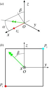
Figure 1. Orientation of the vortex and pressure determination domain information. (a) Vortex orientation and definition of axis. (b) Pressure determination domain. Location of Dirichlet condition indicated by p1. ΔpFOV = p2 − p1.
Download figure:
Standard imageTo simulate the effect that PIV has on the velocity field, noise is added to the velocity field and the resulting velocity field is low-pass filtered such that the noise has the target RMS value around a filtered velocity field without noise. The resulting field of view (FOV) spans a domain of 65 × 65 independent interrogation window sizes (WS) and is captured by a vector field of 257 × 257 vectors, simulating an overlap factor (OF) of 75%. Three different noise field sets are created and are used for all different approaches. By using three different noise field sets and using the same sets for each approach, the likelihood of extreme noise responses is reduced and the relative differences between the approaches are correctly captured.
The pressure gradient is determined by central differences and subsequently integrated with the Poisson solver. A Dirichlet condition (prescribed pressure) is enforced in the lower-left corner (indicated by p1 in figure 1) and Neumann condition (prescribed pressure gradient) is enforced for the rest of the domain boundary.
An extensive parameter space is covered in order to capture the behaviour of the different approaches for likely flow scenarios. An overview of the parameter space covered is shown in table 1.
Table 1. Synthetic assessment parameters.
| Parameter | Values | Unit |
|---|---|---|
| Uc | 0.125, 0.25, 0.5, 1, 2, 4 | WS/Δt |
| Vp | 1, 0.5, 0.25, 0.125 | Uc |
| rc | 1, 2, 4, 8, 16 | WS |
| α | 0°, 30°, 60°, 90° | |
| β | 0°, 45°, 90° | |
| OF | 0, 0.5, 0.75 | |
| u |
0, 0.5, 1, 2, 4 | %Umax |
 |
−5, −1, 0, 1, 5 | %Uc |
An example of synthetic velocity fields is shown in figure 2. The corresponding pressure fields, figure 3, give an indication on how the different approaches perform. The pressure from TR-Volume performs worst, having the largest noise and an asymmetry around the vortex axis. The pressure from TH-Volume shows an improvement having less noise and no asymmetry around the vortex axis. Finally, the result from TH-TR- Stereo seems to give the best results, having the smoothest result and no asymmetry around the vortex axis.

Figure 2. Example of synthetic velocity and vorticity fields. Uc = 2 WS/Δt, Vp/Uc = 0.5, rc = 8 WS, α = 90°, β = 45°, OF = 75%, u = 1% Umax. (a) Streamwise velocity, u. Overlaid are lines of the theoretical pressure starting at 1 WS/Δt with 0.5 WS/Δt steps. (b) Cross-flow velocity, v. (c) Cross-flow velocity, w. (d) Vorticity magnitude,  . Overlaid are lines of theoretical vorticity starting at 0.1 Δt−1 with 0.1 Δt−1 steps.
Download figure:
Standard image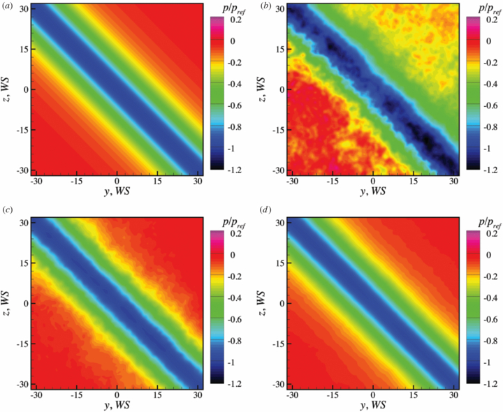
Figure 3. Example of pressure results corresponding to the flow field shown in figure 2. (a) Theoretical pressure. (b) Pressure from TR-Volume. (c) Pressure from TH-Volume. (d) Pressure from TH-TR-Stereo.
Download figure:
Standard imageAt first glance the results confirm the estimates for the noise response found earlier. To quantify the differences and to investigate the asymmetry in the pressure result, which was not expected, the differences between the techniques need to be examined in greater detail.
3.2. Results
For the quantification of the differences between the approaches, three different measures are used. First, to evaluate the amplitude modulation that is introduced by the approach, the peak response, pp/pref, is determined, which is the ratio of the calculated pressure at the vortex centre and the theoretical value. Next, to determine the receptivity to measurement noise, the noise response, p/pref, is determined, which is the RMS of the difference introduced by adding noise to the velocity field. Finally, the difference in pressure estimate across the FOV, ΔpFOV = p2 − p1 (where p1 is the location of the reference pressure, and p2 is the opposite corner of the FOV as shown in figure 1), is determined using the pressure results for the clean velocity fields (without added noise). This difference is calculated in order to quantify the asymmetry in the pressure estimate across the vortex axis (observed in figure 3(b) for a pressure result including velocity noise).
To show the effect of each parameter independently, a non-critical baseline case is taken, around which the parameters are varied. The largest differences were found for the vortex being parallel to the measurement plane. The effect of small angles with respect to the plane normal was investigated by de Kat and van Oudheusden (2012) (albeit for an in-plane convection velocity), and even results from a 2D approach will be sufficient, as can be seen figure 4. The results of the current analysis show no significant changes in their results for these small angles. Therefore, the results of α = 90° will be used to compare the different approaches. Figure 5 shows the results for different spatial resolutions (i.e. WS/rc). As expected, the peak response, figure 5(a), decreases with decreasing resolution (larger WS). TR-Volume and TH-Volume have the same response for OF 75%, and TH-TR-Stereo performs better across most resolutions. For high spatial resolutions (small WS), the performances of all methods are similar. The noise response, figure 5(b), for TR-Volume remains nearly constant over the entire range of spatial resolutions examined. However, the noise response for TH-Volume and TH-TR-Stereo shows a decrease with decreasing spatial resolution. For TR- and TH-Volume, noise increases with increasing OF from 50% to 75%. The asymmetry response, figure 5(c), shows that only the TR-Volume approach is affected for OF 0% and 50%. TR-Volume at OF 75%, all OF for TH-Volume, and all OF for TH-TR-Stereo do not show any asymmetry. The asymmetry for TR-Volume with OF 0% and 50% is due to an additional error introduced by insufficient sampling (for OF 0% Nyquist criterion to resolve spatial structures in velocity is not satisfied; for OF 50% Nyquist criterion to resolve spatial structures in velocity gradient—obtained by central differences—is not satisfied). This additional error results in an imbalance between the temporal and the convective parts of the material acceleration, which manifests itself as an asymmetry in the resulting pressure field. The results in figure 5 indicate that TR-Volume introduces higher levels of uncertainty in both peak and noise responses. This is consistent with our observations based on uncertainty estimates obtained in the previous section.

Figure 4. Peak response with angle to the plane normal, α. Uc = 0.25 WS/Δt, Vp/Uc = 1, rc = 8 WS, β = 45°, OF = 75%,  % Uc.
% Uc.
Download figure:
Standard image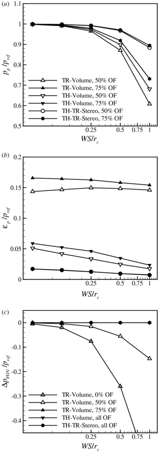
Figure 5. Peak, noise and asymmetry responses with spatial resolution. Unless indicated otherwise: Uc = 0.25 WS/Δt, Vp/Uc = 1, rc = 8 WS, α = 90°, β = 45°, OF = 75%, u = 1% Umax,  % Uc. (a) Peak response. (b) Noise response. (c) Asymmetry response.
Download figure:
Standard imageThe results for different convection velocities are shown in figure 6. The peak response of an Eulerian approach is expected to depend on the temporal resolution with respect to the flow features (see de Kat and van Oudheusden (2012), equation 13). Therefore, the peak response is plotted against UcΔt/rc in figure 6(a). The peak responses for TR-Volume and TH-TR-Stereo show deviations for UcΔt/rc > 0.2. This indicates that both approaches are limited to work only for acquisition frequencies that are sufficiently higher than the Eulerian time scales in the flow (facq > 10 Uc/(2rc) ≈ 10 × fflow). The peak response of the TH-Volume approach is unaffected by changes in convection velocity. The noise response, shown in figure 6(b), scales with the velocity magnitude and is therefore plotted with UcΔt/WS. All approaches show that the noise response decreases with increasing values of UcΔt/WS. The asymmetry response, plotted with UcΔt/rc, shows that for UcΔt/rc > 0.2 only the TR-Volume approach is affected. This is caused by under-resolving the temporal part in the material acceleration, which results in an imbalance between the temporal and the convective parts of the material acceleration, leading to the asymmetry in the pressure field. Figure 7 shows the results for different tangential velocity strengths (i.e. different Vp). Different values of Vp can be interpreted as different turbulence intensity levels. Figures 7(a) and (c) show that there is no influence of the tangential velocity strength on the peak or asymmetry response. However, figure 7(b) shows that the noise response decreases with increasing tangential velocity. This is consistent with the observation of de Kat and van Oudheusden (2012). TR-Volume has the worst performance of the three techniques and shows a larger increase in noise with decreasing tangential velocity than the other two approaches. This means that for low turbulence intensities (small Vp) TH-Volume and TH-TR-Stereo perform even better than TR-Volume than for higher turbulence intensities.

Figure 6. Peak, noise and asymmetry responses with convection velocity. Unless indicated otherwise: Uc = 0.25 WS/Δt, Vp/Uc = 1, rc = 8 WS, α = 90°, β = 45°, OF = 75%, u = 1% Umax,  % Uc. (a) Peak response. (b) Noise response. (c) Asymmetry response.
Download figure:
Standard image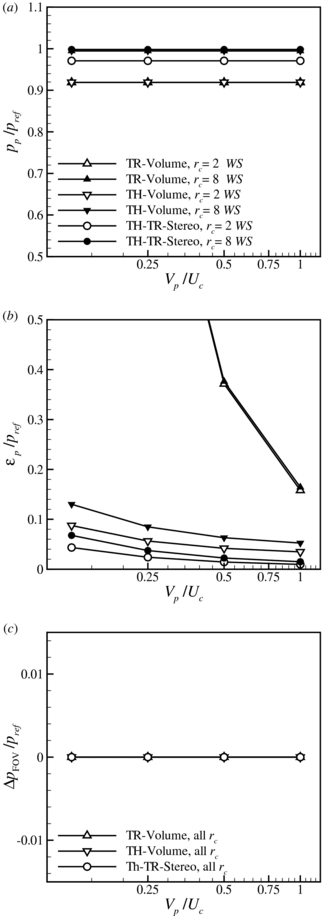
Figure 7. Peak, noise and asymmetry responses with tangential velocity. Unless indicated otherwise: Uc = 0.25 WS/Δt, Vp/Uc = 1, rc = 8 WS, α = 90°, β = 45°, OF = 75%, u = 1% Umax,  % Uc. (a) Peak response. (b) Noise response. (c) Asymmetry response.
Download figure:
Standard imageThe noise response as a function of noise on the velocity field is shown in figure 8 and shows that pressure noise is increasing linearly with increasing velocity noise. For all cases it was found that the noise levels for TR-Volume are the highest, TH-Volume performs better with lower noise levels and TH-TR-Stereo always shows the lowest noise levels.
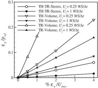
Figure 8. Influence of velocity error, u, on the noise response. Uc = 0.25 WS/Δt, Vp/Uc = 1, rc = 8 WS, α = 90°, β = 45°, OF = 75% and  % Uc.
% Uc.
Download figure:
Standard imageThus far, we have examined the performance of Taylor's hypothesis approaches assuming that the convection velocity is already known. However, in most applications, this is not necessarily true. Therefore, we examine the effect of uncertainty in convection velocity on pressure estimation. Figure 9 shows the influence of an error in the convection velocity on the peak and asymmetry response. Both peak and asymmetry response are affected. For TH-Volume, the change in peak response is affected to a lesser extent than the asymmetry response, whereas for TH-TR-Stereo both the peak and asymmetry response are similar.

Figure 9. Influence of convection velocity error,  , on the peak and asymmetry response. Uc = 0.25 WS/Δt, Vp/Uc = 1, rc = 8 WS, α = 90°, and β = 45°, OF = 75%.
Download figure:
Standard imageThe results from the synthetic data performance assessment show that if the convection velocity is known, the determination of pressure in convective flows can be significantly improved by using this information for a modified Eulerian approach.
Even if the convection velocity is not exactly known, the new approach can outperform TR-Volume, provided the combined error due to convection velocity and velocity noise is small. This is likely for turbulent flows with low turbulence intensities. For these flows, the convection velocity is likely to be close to the mean velocity, and, therefore, the error due to the convection velocity is small.
Assuming a flow with a turbulence intensity of  , i.e.
  , that is properly sampled (no peak response issues) with a velocity error of 1%Umax, the error on the pressure field would be around 20% with TH-Volume and slightly better with TH-TR-Stereo. However, if TR-Volume were to be used, the error on the pressure field would be in excess of 100%.
It must be noted that in all the comparisons made here, we did not take differences in velocity measurement accuracy into account between the different techniques. Volumetric techniques generally have a larger uncertainty on the velocity measurement than planar techniques, e.g. tomographic PIV has typically 0.2–0.4 voxels/pixels error in the correlation (Elsinga 2008, Worth et al 2010, Atkinson et al 2010), whereas planar PIV has typically 0.1 pixels error in the correlation (Nobach and Bodenschatz 2009). This means that TH-TR-Stereo will be more accurate than is depicted by this analysis on synthetic data.
This gives us confidence that the new approach can provide useful and accurate pressure estimates if the convection velocity is known within reasonable accuracy. Therefore, we apply this method to experimental data obtained in a turbulent jet flow.
4. Pressure fluctuations in a turbulent jet
To illustrate the capabilities of this technique, it is applied to the far field of a turbulent jet, as measured by Ganapathisubramani et al (2007), who applied cinematographic stereo PIV (i.e. time-resolved stereo PIV). A brief summary of important experimental details and flow characteristics is given in table 2.
Table 2. Experimental characteristics (Ganapathisubramani et al 2007, 2008).
| Flow characteristics | |
|---|---|
| Jet Reynolds number, ReD | 5,100 |
| Turbulence intensity at measurement location | ≈30% |
| Jet half-width, δ1/2 | 126 mm |
| Taylor microscale, λ, at measurement location | 13.8 mm |
| Kolmogorov scale, η | 0.52 mm |
| Typical vortex diameter, dv | 10η |
| Typical vortex radius, rv = dv/2 | 5η |
| PIV details | |
| Field of view, FOV | 76 × 76 mm2 |
| Acquisition frequency (image pairs), facq | 1 kHz |
| Velocity field time separation, Δt = 1/facq | 1 ms |
| Final interrogation window | 16 × 16 pixels |
| 1.35 × 1.35 mm2 | |
| Overlap factor, OF | 50% |
Using the TH-TR-Stereo approach, pressure is determined using the mean velocity as the convection velocity, Uc = U. This convection velocity varies in the cross-flow direction as shown in figure 10, ranging from approximately 0.4 to 0.8 m s−1. For this experiment, the spatial resolution with respect to the typical vortices in the flow is 0.6 WS/rv, where rv is the radius of a typical vortex (see table 2). The convection velocity range is Uc ≈ 0.3–0.6 WS/Δt = 0.2–0.3 rv/Δt, and the tangential velocity can be estimated as three times the turbulence intensity, Vp/Uc ≈ 0.9. Based on the synthetic data analysis these values should give good pressure results, provided that the mean velocity is the right convection velocity. Figure 11 shows an example of the result. Figure 11(a) shows the instantaneous velocity field, figure 11(b) shows the instantaneous vorticity magnitude field. When comparing the two figures, different vortex orientations can be observed. Two sets of vortices are indicated: one set with vortices that have primarily in-plane vorticity, indicated by A, and one set with vortices that have primarily out-of-plane vorticity, indicated by B. The pressure is determined with respect to the top-right corner, indicated by the red dot. Figure 11(c) shows the corresponding pressure field. The pressure across the in-plane vortices, indicated by A, shows an asymmetry, having a significantly lower pressure away from the reference point. The pressure around the out-of-plane vortices, indicated by B, does not show this behaviour. Similar asymmetry in the pressure field for an in-plane vortex travelling through the measurement plane was observed for TR-Volume in figure 3; however, from a single pressure field it is hard to see whether this is flow or technique related. The time evolution of the pressure at the reference location was determined by directly integrating the pressure in the axial direction, and is shown in figure 11(d). This point was chosen for its relative low mean axial velocity (i.e. best temporal resolution with respect to the flow) and for the low levels of vorticity at this point. The time evolution of the pressure at this reference point is now used to create a space–time volume to visualize the relation between the pressure and the flow structures, see figure 12.
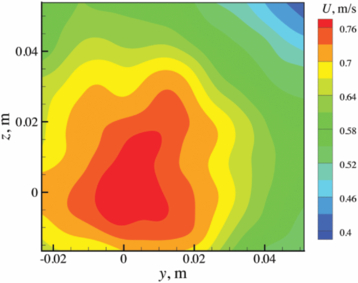
Figure 10. Mean axial velocity distribution in the measurement plane (data reproduced from Ganapathisubramani et al 2007).
Download figure:
Standard image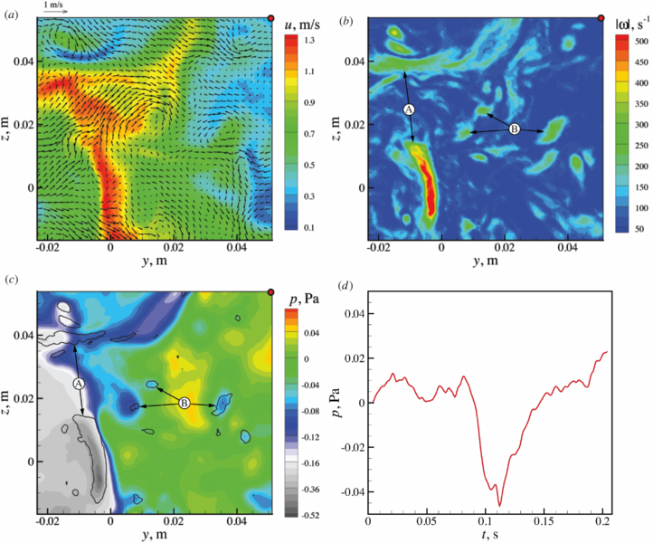
Figure 11. Instantaneous velocity and pressure fields at t = 0.022 s for Uc = U. The red dot indicates the location of the reference pressure point. (a) Velocity field. Colour isocontours of u. Vectors show in-plane velocity, v and w. Each third vector is shown in the y- and z-directions. (b) Vorticity magnitude field,  . (c) Pressure field (below −0.16 Pa, the colour scale step size changes). Overlaid black lines indicate
  s−1. (d) Time evolution of the pressure at the reference point.
Download figure:
Standard image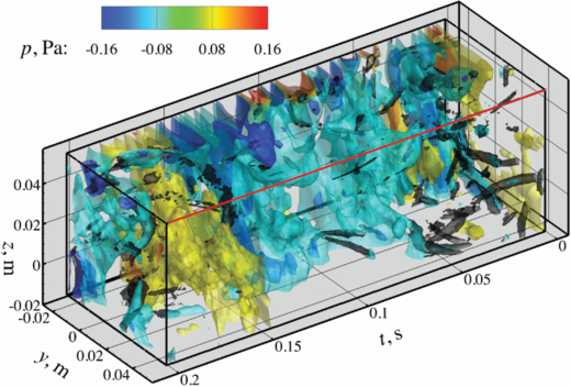
Figure 12. Space–time volume of pressure, Uc = U. The location of the reference pressure, see figure 11(d), is depicted by the red edge. Isocontours of vorticity magnitude ( s−1) are shown in black. Isosurfaces of pressure are shown for −0.16 , −0.08, 0.08 and 0.16 Pa.
Download figure:
Standard imageThe space–time pressure volume in figure 12 shows strong oscillations on the far side(s) of the reference pressure. They are clearly visible along the top edge opposite to the reference point. The oscillations are related to in-plane vortices passing through the measurement plane, see figure 11(c), and can be explained as asymmetries that are introduced by using an incorrect convection velocity as also seen and quantified in figure 9 in section 3.
The uncertainty on the convection velocity can be estimated using the RMS pressure fluctuations in the corner away from the reference point with respect to a typical pressure inside a vortex. Figure 9 shows that ΔpFOV and Δpp are similar for TH-TR-Stereo. Using this information, we can estimate the peak pressure difference that the lower in-plane vortex (marked A) will introduce into the pressure field by pv ≈ |pA − pcorner| = 24 mPa, where pA is the peak pressure measured within the vortex and pcorner is the pressure measured in the lower-left corner. This vortex was the strongest in-plane vortex found to pass the measurement plane. If we consider this to be the maximum pressure perturbation, the RMS value of the pressure fluctuations in the corners should be lower. Taking the RMS fluctuation of the three corners with respect to the reference point we find (pcorners)RMS = 131 mPa, which is significantly larger than what is expected. Estimating the asymmetry error to be the surplus of (pcorners)RMS with respect to pv, it follows that (ΔpFOV)RMS/pv ≈ 4.5. For this value of asymmetry error, the estimate for the RMS error in convection velocity is 150%, which is obtained by extrapolating the straight line in figure 9. It should be noted that this estimate for the error in convection velocity is a worst-case estimate, as it is estimated from the signal without knowledge of what is signal and what is error. Moreover, the error includes random error as well as convection velocity error. Therefore, the real error in convection velocity is likely to be smaller. However, given the current dataset there is no better way to estimate it. Nevertheless, the estimate of the error on the convection velocity supports the idea that using the mean as the convection velocity for pressure determination may not be correct.
In order to try to overcome this problem, a different way of estimating the convection velocity is to be used. The instantaneous axial velocity is filtered in-plane by a moving average over a kernel with sides lf to obtain the estimate for the convection velocity, [u]. It should be noted that this approach to estimate the convection velocity may seem arbitrary; however, similar (more elaborate) methods have been successfully applied, e.g., by Davoust and Jacquin (2011). Moreover, Elsinga et al (2012) found, by tracking hairpin structures in a turbulent boundary layer, that the difference between the local flow velocity and the convection velocity is smaller than the difference between the mean velocity and the convection velocity. To examine how different filter sizes affect the input to the pressure solver, the relative change of the divergence of the velocity field and the relative change of the curl of the in-plane pressure gradient are determined. Ideally, both of these values are zero; however, due to measurement errors they will have a certain spread. Figure 13 shows the result of this analysis. The positive change in divergence indicates that there is less agreement in terms of continuity. This amount of change decreases with increasing lf. Even though the result is worse in terms of continuity, the change in curl of the in-plane pressure gradient is negative, which means the resulting pressure gradient is better. The error in curl is 23% lower up to lf = 10 mm. Near the smallest value (smallest value means no filter, which is equal to a 2D approach) the change is slightly smaller. Similar results were found for a moving average in time and for a moving average in space and time.
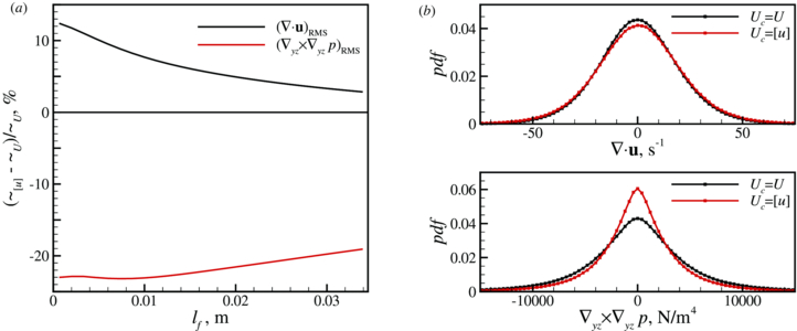
Figure 13. Filter length determination. (a) Influence of filter length on  and ∇yz × ∇yzp; (b) pdfs of
  and ∇yz × ∇yzp for lf = 10 mm.
Download figure:
Standard imageTo obtain the largest improvement for the curl with the smallest deterioration in the divergence, lf = 10 mm is used, which corresponds to twice the typical vortex tube diameter (Ganapathisubramani et al 2008). Probability density functions (pdfs) for this filter length, figure 13(b), show that there is a large improvement in curl and a (relatively) smaller deterioration in divergence. Even though this approach to estimate convection velocity deteriorates continuity, the reduction in error for the pressure gradient is evident. As the goal is to get a better estimate for the pressure field, this deterioration of continuity is of less importance than the improvement of the pressure gradient input.
For this convection velocity, the spatial resolution and the estimated peak tangential velocity remain the same; however, the convection velocity now has a range of Uc ≈ 0.1–0.9 WS/Δt = 0.05–0.5 rv/Δt. These values should still give good pressure results based on the synthetic data analysis, provided the new estimates for convection velocity are better. Figure 14 shows the results for Uc = [u]. The velocity field in figure 14(a) is identical to the field in figure 11(a). The vorticity field in figure 14(b), however, used the streamwise velocity gradients calculated using the new convection velocity. The figure shows that there is very little change compared to figure 11(b). However, the pressure field in figure 14(c) shows substantial differences compared to figure 11(c). The pressure on the right-hand side of the FOV is very similar between these figures (regions around vortices marked as B); however, the pressure on the left-hand side is substantially different, especially the notable absence of asymmetry across the vortices marked A. This supports the idea that the asymmetry that was obtained by using the mean velocity as the convection velocity in figure 11(c) is an artefact of a mismatch in convection velocity of this vortex A. However, the use of a local convection velocity (obtained through in-plane filtering of the instantaneous streamwise velocity) provides a 'better' estimate of the convection velocity of the vortex A, thereby minimizing the asymmetry. Figure 14(d) shows the time evolution of the reference pressure compared to the results of Uc = [u]. The general trends of the reference are similar, but there are differences in magnitude. Again, this difference in magnitude can be attributed to a 'better' estimate of the local convection velocity. Figure 15 shows the resulting space–time pressure volume. The strong oscillations have disappeared and collocated low pressure and high vorticity can be seen at the top of the volume, whereas in figure 12 there was no clear link between the vorticity and pressure. The volume shows large regions of high and low pressure with strong vortices piercing through these regions creating locally lower pressure.
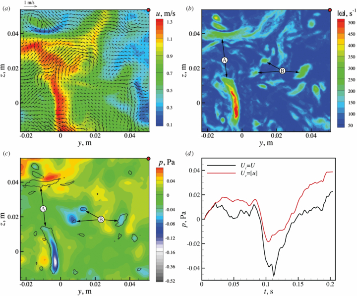
Figure 14. Instantaneous velocity and pressure fields at t = 0.022 s for Uc = [u]. The red dot indicates the location of the reference pressure point. (a) Velocity field. Colour isocontours of u. Vectors show in-plane velocity, v and w. Each third vector is shown in the y- and z-directions. (b) Vorticity magnitude field,  . (c) Pressure field (below −0.16 Pa, the colour scale step size changes). Overlaid black lines indicate
  s−1. (d) Time evolution of the pressure at the reference point.
Download figure:
Standard image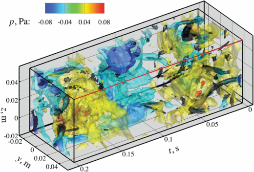
Figure 15. Space–time volume of pressure for Uc = [u]. The location of the reference pressure, see figure 14(d), is depicted by the red edge. Isocontours of vorticity magnitude ( s−1) are shown in black. Isosurfaces of pressure are shown for −0.08, −0.04, 0.04 and 0.08 Pa.
Download figure:
Standard imageUsing the same method to estimate the error on the convection velocity as before, we find pv ≈ pA − pcorner = 22 mPa, which is in good agreement with the estimate found for Uc = U, and supports the idea that this is a good estimate for the pressure perturbation introduced by the lower in-plane vortex marked by A. Taking the RMS fluctuation of the three corners with respect to the reference point, we find  mPa, which is close to what is expected. From this it follows that (ΔpFOV)RMS/pv ≈ 1.6. The estimate of the RMS error in the convection velocity now becomes approximately 20%. Again, it should be noted that this estimate for the error in convection velocity is a worst-case estimate, as it is estimated from the signal without knowledge of what is signal and what is error. Moreover, the error includes random error as well as convection velocity error. Therefore, the real error in convection velocity is likely to be smaller. This error estimate confirms that in this flow the new estimate for convection velocity is better than using the mean velocity as convection velocity for pressure determination.
The results show that the mean velocity is not the correct convection velocity for this flow, as evidenced by the oscillations/asymmetries and estimated error on the convection velocity. This is not unexpected, since Taylor's hypothesis only holds for flows where the turbulent fluctuations are small. In the jet, the turbulent fluctuations are significant (≈30%). In this situation, there is most likely a range of convection velocities. The improvement when using a filtered instantaneous velocity as convection velocity (even though this still is not the correct convection velocity) suggests that if the convection velocity can be determined within reasonable accuracy, the pressure can be determined using the Taylor's hypothesis pressure determination approach.
In any case, it is not possible to validate the pressure estimates in this flow. The levels of pressure fluctuations (< 0.2 Pa) are too small to be captured with pressure transducers. To our knowledge, the uncertainty of a specialized commercially available pressure transducer after specific calibration is approximately ±0.3 Pa (e.g. Endevco 8507C-1, see de Kat and van Oudheusden 2012) and will therefore be unable to capture the instantaneous fluctuations observed in this study. Microphones are more sensitive and could be able to capture these small levels of fluctuation. However, the microphones that are able to capture the frequency range and levels of pressure fluctuations accurately are at least 1/2 inch in diameter (e.g. Brüel and Kjaer microphone type 4188), which means that they would only be able to capture spatial fluctuations larger than 50 mm. In the current flow, this corresponds to a spatial resolution of about 4λ (where λ is the Taylor microscale).
Furthermore, application of a TR-Volume technique for the current problem would result in larger errors than estimated for the TH-TR-Stereo, ranging from 210% to 40% (based on the synthetic data analysis for WS = 2rv, Uc = 0.125–1 WS/Δt, Vp/Uc = 1 and u = 4%). Applying a Lagrangian approach combined with time-resolved volumetric PIV will improve the random noise response at best by a factor of 2 (optimistic estimate for the improvement based on the region where Uc < 1 WS/Δt in figure 4(e) from de Kat and van Oudheusden (2012)). Apart from difficulties that are associated with implementing this technique (e.g. large volumes needed at high spatial resolution), the improvement of applying a Lagrangian technique would at best make it on a par with the error from TH-TR-Stereo in its current implementation.
This suggests that TH-TR-Stereo is the only way to accurately determine pressure fluctuations for turbulent convective flows, provided that an appropriate estimate for the convection velocity can be obtained.
5. Conclusions
In this paper, a new approach for pressure estimation in convective flows is proposed. The approach combines volumetric or time-resolved cross-plane measurements with Taylor's hypothesis to calculate pressure.
Based on theoretical estimates and performance assessment on synthetic data it is found that, if the convection velocity is known, this new method is easier to apply and less prone to errors than previous available techniques. The TH-TR-Stereo approach typically outperforms a TR-Volume approach by an order of magnitude in noise response.
Application of the new approach on time-resolved data in the cross-flow plane of a turbulent jet shows that, in this case, the mean velocity is the incorrect convection velocity for pressure determination and that a local convection velocity estimate (in-plane filtered axial velocity) reduces the error on the pressure gradient significantly and gives more realistic pressure results.
All the results appear to indicate that, when applied appropriately, the new approach can be used to determine pressure fluctuations in turbulent convective flows, where, due to their small amplitude and spatial extent, there are no other means to determine pressure fluctuations.
Acknowledgment
We gratefully acknowledge the support from UK Engineering and Physical Sciences Research Council (EPSRC) through grant EP/I004785/1.