

Abstract
We discuss the challenges and limitations associated with the development of a large field of view particle image velocimetry (LF-PIV) diagnostic, capable of resolving large-scale motions (>1 m per camera) in gas phase laboratory and field experiments. While this diagnostic is developed for the measurement of wakes and local inflow conditions around research wind turbines, the design considerations provided here are also relevant for the application of LF-PIV to atmospheric boundary layer, rotorcraft dynamics and large-scale wind tunnel flows. Measurements over an area of 0.75 m × 1.0 m on a confined vortex were obtained using a standard 2MP camera, with the potential for increasing this area significantly using 11MP cameras. The cameras in this case were oriented orthogonal to the measurement plane receiving only the side-scattered component of light from the particles. Scaling laws associated with LF-PIV systems are also presented along with the performance analysis of low-density, large diameter Expancel particles, that appear to be promising candidates for LF-PIV seeding.
Export citation and abstract BibTeX RIS
Symbols
| ρp | Density of a flow tracking particle ( ) ) |
| dr | Pixel pitch of recording medium (m) |
| dτ | Image diameter as recorded by the recording medium (m) |
| Lx | Linear dimension of the recording medium (m), e.g. CCD chip size |
| Nx | Number of pixels in recording medium in the x-direction |
| Mo | Magnification of the imaging system |
| ΔXp, max | Maximum displacement of particle on the recording medium (m) |
| Δx | Variable displacement vector |
| p | Overlap ratio of interrogation region |
| ΔXpixI | Size of interrogation region (pixels) |
| ΔXI | Size of interrogation region (m) |
| wo | Laser light beam waist (minimum thickness) (mm) |
| w | Laser light beam diameter (mm) |
| δw | Laser light beam divergence (mrad) |
| Rao | Rayleigh length of light sheet (m) |
| Ω | Solid angle subtended by the lens aperture at a particle at the center of the measurement plane |
| Da | Diameter of lens aperture (m) |
| f | Focal length of lens (mm) |
 |
f number (aperture size) |
| Jo | Total energy in light pulse (J) |
| dp | Diameter of particle (m) |
| zo | Object distance (m) |
| Zo | Image distance (m) |
| λ | Wavelength of light (m) |
| Δyo | Height of the light sheet (m) |
| Δzo | Thickness of the light sheet (mm) |
| q | Scattering exponent power (2 < q < 4) |
| τo | Time constant (μs) |
| g | Acceleration ( ) )
|
| C | Particle density (per  ) )
|
| N | Number of particles |
| V | Given volume ( ) )
|
| ξ | Number of particle-image pairs available for a PIV estimate |
| Δt | Inter-frame time delay (μs) |
| F, G | Unknown functions |
| σw | Out-of-plane fluctuations in velocity (m s−1) |
1. Introduction
Particle-image velocimetry (PIV) measurements thus far have generally been constrained to the study of small-scale flows or small regions in large-scale flows due to field of view (FoV) limitations (Raffel et al 2007, Adrian and Westerweel 2010). And yet, several problems of practical interest such as flows around wind turbines and planetary boundary layers (PBL) involve large flow fields. Currently, these flow fields are measured using either single point diagnostics (e.g. sonic anemometry) or scanning techniques with low spatial resolution and accuracy (e.g. Lidar, Sodar). As a consequence, important dynamics of the turbulent flow field is not completely understood. In wind turbine research, measurements of the statistics and spatial structure of inflow turbulence are lacking due to the absence of a non-intrusive measurement method, such as PIV. In PBLs, the correlations of the near-wall turbulence, the organization of coherent structures and spatial structure of the turbulence can all be studied using a non-intrusive and accurate multi-point measurement diagnostic. The measurement of large-scale flow fields also become important in light of recent findings about the energetic contents of large-scale motions (Kim and Adrian 1999, Guala et al 2006, Balakumar and Adrian 2007, Hutchins and Marusic 2007, Monty et al 2007).
In this work, we discuss the design of a large field of view particle image velocimetry (LF-PIV) system that is capable of resolutions of less than 1 mm/pixel. The performance and flow tracking fidelity of LF-PIV is analyzed by testing this system on a laboratory-scale tank with a 1.2 m × 1.2 m cross-section capable of generating and sustaining a turbulent confined vortex. Recently, PIV measurements with a large FoV have been performed in the wind tunnel to study rotorcraft aerodynamics (Silva et al 2004b, 2004a, Yamauchi et al 2011) and spread of fires inside enclosures (Bryant 2009). These two projects used different seed particles (olive oil versus Expancel particles) and demonstrated PIV FoVs of up to 1.1 m × 4.3 m (using overlapping fields of view) and 1.7 m × 2.3 m (using stereo-PIV), respectively. LF-PIV has also been performed by padding images from several cameras to obtain detailed flow measurement over a large area as shown in Carmer et al (2008). Usage of novel tracers such as helium filled soap bubbles as tracer particles has permitted to expand FoVs in orders of several meters (Bosbach et al 2009). Despite the gradual proliferation of LF-PIV, several aspects regarding the accuracy and performance of these systems remain unresolved. In this paper, we will address some of these issues (including flow tracking fidelity, light-sheet design, scaling of light scattering from particles) by performing experiments on a laboratory-scale apparatus. In the future, the diagnostic is expected to be fielded to study wind turbine inflow and wake on 4.5 m turbines at the Los Alamos National Laboratory's wind turbine field station.
2. Experimental setup
A large 1.2 m × 1.2 m × 0.6 m tank with transparent glass walls was constructed to test the performance of the LF-PIV diagnostic. A cylindrical cross-flow blower was installed at a bottom corner of the tank to generate a large vortex inside the tank (figure 1). Speed-control on the blower allowed the tuning of the tangential velocity of the vortex. There were four drivers for the selection of this apparatus for the development of LF-PIV: (a) the apparatus allowed the control of the tangential velocity and hence the centrifugal accelerations that the particles are subjected to, (b) the vortex tank replicates the turbulent tip vortices shed by wind turbine blades and offers a laboratory-scale test bed prior to their application in wind energy (our current interest), (c) the ability to test different particles within a confined space in the laboratory and (d) scalability of the apparatus. Based on the size of the apparatus, a maximum FoV of 1.2 m × 1.2 m can be achieved. However, the apparatus itself could be moved across the laser light-sheet using a hydraulic lift table. This allowed the transport of the flow itself to a particular region of the camera's FoV while keeping the light sheet fixed.

Figure 1. Schematic of the large field of view particle image velocimetry setup on a laboratory scale vortex generated inside a tank filled with air.
Download figure:
Standard imageLight-weight (ρp = 30 kg m−3) acrylic copolymer particles of mean diameter 80 μm (Expancel microspheres from AkzoNobel) were used to seed the flow. The particles were introduced through an opening near the top of the tank, and were vacuumed out after the completion of the experiment. Since the particles are unpleasant to inhale in large concentrations, several HEPA filters were located near the apparatus to keep the ambient air clean. It is important to note that the large particles significantly improve the scattered light signal from the particles recorded by the LF-PIV camera. However, the low density of the particles ensures that they track the flow significantly better than solid particles of the same diameter. Thus, Expancel particles present a good alternative to olive oil droplets for LF-PIV measurements (Adrian 2011, Bryant 2009), although olive oil has also been used successfully for LF-PIV measurements in large wind tunnel experiments (Silva et al 2004b).
The flow field was illuminated using a dual-head Nd:YAG laser (Quantel USA) with a measured output power of 200 mJ/pulse. The near field beam thickness was  , the duration of each laser pulse
  and beam divergence
  . The output beam was shaped into a wide sheet using a conventional optical arrangement. The optical arrangement included a spherical lens of focal length
  to reduce the beam thickness and hence the light sheet thickness at the measurement plane. A plano-concave cylindrical lens of focal length
  to shape the beam into a sheet. This simple arrangement was found to be adequate to illuminate the current flow field; however, a more complex arrangement with telescopic lenses or beam expanders could be used to contain the beam thickness at larger distances of the measurement plane from the head of the laser.
The light scattered from the particles was recorded using standard 2MP PIV cameras (TSI Inc., Powerview Plus) with a CCD size of 1192 × 1600 pixels, a pixel pitch of 7.4 μm and a 12-bit output used in side-scatter mode. Different focal length lenses (Nikon Nikkor  and
and  ) were used depending on the desired FoVs. For LF-PIV measurements, large depths of field were achieved due to the small magnifications involved. This allowed the operation of the camera at large apertures (
 ) resulting in maximum light collection. For small FoV PIV (referred to as SF-PIV in this paper), the aperture size was reduced (
 ) to ensure that particles illuminated by the light sheet are in focus.
In order to determine the performance differences between LF-PIV and conventional SF-PIV, experiments were performed using two different FoVs of  and
and  (SF-PIV1), respectively. The LF-PIV camera was placed at a stand-off distance of 5 m and the SF-PIV camera was placed 0.9 m away from the measurement region. The PIV images were obtained at 5 Hz, and all triggering signals were generated using Stanford Research Systems digital delay generators. The inter-frame interval was selected to be 1500 μs for LF-PIV and 250 μs for the SF-PIV measurements. The statistics presented for this comparison were obtained from 1000 image pairs. A convergence study showed this ensemble to be sufficient for the measurement of converged mean (difference less than 1%) and standard deviation (difference less than 2.5%). The particle Stokes number varied between 10−4 and 10−3 for a range of dissipation values within the turbulent flow in the tank. This is less than the recommended maximum value of 10−2 for particle tracking fidelity (Salazar and Collins 2009).
Further, to test the flow tracking ability of the Expancel particles a comparison study was performed between the measurements obtained using Expancel particles and typically used theatrical fog droplets (henceforth referred to as fog particles). To avoid uncertainty in the measurements due to increasing FoV, this comparison was performed for an FoV size of  (SF-PIV2 and SF-PIV3). The statistics presented for this comparison were obtained from 2500 image pairs with inter-frame interval of 150 μs.
3. LF-PIV design considerations
The large stand-off distances between the measurement plane and the recording device (CCD camera) along with small particle sizes required for the measurement of gaseous flows pose several challenges for the successful design of an LF-PIV experiment. In this section, we will discuss the various design parameters that must be considered for optimizing the quality of LF-PIV measurements. We will begin by considering the three approaches that can be used for increasing the FoV of a standard PIV setup.
3.1. Dynamic measurement range
The FoV of a camera (defined as the size of the measurement plane recorded by the imaging system) is given by
Thus, the FoV can be increased by increasing the number of pixels on a CCD chip (Nx), by increasing the size of the pixels in a given CCD (dr) or by reducing the magnification (Mo). In turn, the magnification can be reduced by the use of a wide-angle lens or by increasing the stand-off distance between the camera and the measurement plane.
The effect of each of these approaches on the quality of the measurements can be understood by considering the ratio of the scales of the velocity spatial spectra as measured by a PIV system and the dynamic velocity range (DVR). The former parameter is used here instead of the standard dynamic spatial range (DSR) (Adrian 1997) as we are not using super-resolution PIV. In our case, the smallest spatial velocity fluctuation that can be measured is between adjacent vectors. This parameter (henceforth called the dynamic length scale ratio, DLSR) is defined as the ratio of the largest to the smallest spatial scale in the velocity spectrum that can be measuring using LF-PIV. The largest measurable wavelength of the velocity variation is given by the projection of the format of the imager (linear dimension of the CCD) on the measurement plane. This is approximately the farthest distance between the vectors in a PIV vector field. The smallest wavelength is given by the distance between adjacent vectors in the same field. The ratio of these scales (DLSR) is given by
Thus, increasing the number of pixels in a CCD increases the DLSR and allows the measurement of a wider range of scales while simultaneously increasing the FoV. On the other hand, increasing FoV by reducing the magnification or increasing the pixel pitch has no effect on the measured range of scales. It is often more practical and cost-effective to use a wide angle lens to increase the FoV than to increase the CCD size. In these cases, we sacrifice some of the information contained in the smaller scales of motion to measure the larger scales. The effect of this compromise is discussed in a subsequent section by considering a confined turbulent vortex flow experiment.
The ratio of the largest to the smallest velocity that can be measured by a PIV system is called the DVR and is given by (Adrian 1997)
Typical LF-PIV systems are diffraction limited due to the small magnifications involved, and the diameter of the particle image on the imager is smaller than the pixel pitch (i.e. the recorded images of the small particles on a CCD are one pixel in size). This conclusion can also be obtained by formally calculating the diffraction limited spot size and following the equations in Adrian (1997). Thus, for a given interrogation scheme and a fixed maximum inter-frame displacement of the particles on the imager (ΔXp, max), the DVR remains fixed. Thus, increasing FoV by increasing the pixel pitch, increasing the total number of pixels or reducing the magnification has no effect on the DVR.
In summary, the most optimal method of recording LF-PIV images is by increasing the number of pixels in the imager. This results in a gain in both the FoV and the DLSR. An inferior (but often more practical and cost-effective) alternative is to reduce the magnification of the PIV system. In this case, the largest scales are measured at the expense of the smaller scales. In all three cases, the dynamic velocity range remains fixed.
3.2. Laser light sheet properties for LF-PIV
It is well known that coherent beams from Nd:YAG lasers do not follow conventional ray optics. Instead, they are designed to follow Gaussian beam optics (Adrian and Westerweel 2010), and form a waist region of minimum thickness after passing through a converging optic. As a consequence, the laser light sheets used in PIV are non-uniform over the measurement region. While this non-uniformity is usually not a concern in conventional PIV systems due to the small FoVs, it is useful to understand the design rules necessary in LF-PIV systems to create light sheets that are not excessively non-uniform. The total length over which the width of a coherent beam remains within  times the minimum waist of the beam (2wo) is given by twice the Rayleigh length (also called the beam depth of focus) (Adrian and Westerweel 2010):
The dependence of the Rayleigh length on the square of the waist thickness is important, as a ninefold increase in the Rayleigh length can be obtained by merely tripling the waist thickness (corresponding to a three-fold reduction in scattered light). However, typical high power laser beams that may be required for LF-PIV do not have a perfect Gaussian intensity profile. In this case, the Rayleigh length is reduced significantly. To ensure that laser beam thickness remains reasonably small, beam divergence reducing optics such as beam expanders may be used. This will lead to thicker light sheet as compared to a typical PIV arrangement; however, this may be beneficial for LF-PIV systems to avoid out-of-plane bias errors.
Further, the divergence angle corresponding to the expansion of the beam to a sheet (not the laser beam divergence δw) will eventually reduce the intensity of the laser sheet, thereby affecting the ability of the camera to image particles. It is possible to reduce the expansion angle by using a larger diameter lens or a Fresnel lens (placed at appropriate distance and focal length) so that the sheet width can be held nearly constant. Further, by having PIV cameras side by side, a linear increase in the FoV can be obtained (under the condition that the beam divergence does not increase the diameter of the beam that significantly reduces the intensity of the light sheet).
3.3. Effective particle exposure
We showed earlier that reducing the magnification of an optical system by increasing the stand-off distance of the camera from the measurement plane is a practical method of increasing FoV. However, increasing the stand-off comes at the expense of reducing the solid-angle subtended by each particle that is imaged by the camera, causing a reduction in the scatter signal recoded from the particles. For a particle located at the center of the measurement plane, this reduction is given by
For small magnifications (typical in LF-PIV), the fraction of scattered light reaching the lens is proportional to the square of the magnification. The effective exposure of a particle image for diffraction limited imaging systems is given by (Adrian 1991, Adrian and Westerweel 2010)
As an illustration, figure 2 shows images of the same area in the object plane having different FoVs. These images were obtained using two different cameras; however, they were synchronized with the laser light to allow for in situ imaging. Further, both the cameras were pointing to the same location in the object plane. The image on the left was obtained using the camera that had lens f = 120 mm and Zo = 0.38 m leading to an FoV:  . The image at the right was obtained using the camera that had lens f = 105 mm and Zo = 0.8 m leading to an FoV:
  . The image obtained at a smaller FoV is brighter as compared to the image at a larger FoV. The enlarged image with a smaller FoV clearly shows bright particle image spots; however, such spots cannot be seen in the enlarged image having the larger FoV.

Figure 2. Particle images obtained at different FoVs. The particle image intensity is much higher for the image with smaller image FoV (image to the left).
Download figure:
Standard imageFor a given aperture diameter (Da) and a given light-sheet thickness, let us consider the effect of increasing the scale of the experiment by a factor m. It was argued in Adrian and Westerweel (2010) that the effective exposure would reduce by a factor of m5 if the particle diameter is kept constant. However, as discussed earlier, LF-PIV systems increase the stand-off distance to lower the magnification and gain FoV. The image and object distances are given by
Therefore, the product Z2ozo2 in the denominator of equation (6) scales as
For LF-PIV, the laser light sheet must increase in scale by a factor of m. Therefore, for a fixed focal length lens, increasing the stand-off distance to reduce Mo by a factor of m results in a reduction in the effective exposure by a factor of m3. It is quite impractical to increase the laser energy to offset this reduction. For example, increasing the FoV by a factor of m = 6 would require a 43 J/pulse laser instead of a 200 mJ/pulse laser! Two other promising avenues also exist to increase exposure. The first is the imaging of particles in forward scatter (Yamauchi et al 2011, Adrian 2011). This would require distortion corrections on the recorded images. Another possibility is the use of larger diameter, low-density seed particles. For the same gain in the FoV, this would require the use of 15 μm particles to maintain the effective exposure.
3.4. Flow tracking fidelity
The use of larger particles invariably results in greater slip between the fluid and the particle. For small particle slip Reynolds numbers, the slip velocity is calculated as (Adrian and Westerweel 2010)
where τo is a time constant denoting the ratio of inertial and viscous forces. The finite particle slip Reynolds number correction, ϕ, is calculated using empirical relationships as detailed in Adrian and Westerweel (2010). The particle slip for a given flow field velocity and acceleration is then calculated using an iterative procedure. It is instructive to examine the performance of Expancel particles in contrast to conventional olive oil particles. Table 1 presents the particle time constants and slip velocities for Expancel and olive oil particles.
Table 1. Performance comparison of Expancel versus olive oil droplet particles for two representative LF-PIV cases.
| Particle type | Time constant (τo in μs) | % slip for g ∼ 20 m s−2 Vortex diameter = 0.4 m Tangential speed = 2 m s−1 | % slip for g ∼ 1000 m s−2 Vortex diameter = 2 m Tangential speed = 32 m s−1 |
|---|---|---|---|
| Expancel | |||
| dp = 80 μm | 472.4 | 0.450% | 1.15% |
| dp = 15 μm | 16.6 | 0.016% | 0.04% |
| Olive oil particle | |||
| dp = 1 μm | 2.4 | 0.002% | 0.01% |
It is clear that even in the case of a moderately intense vortex (with accelerations reaching  ), the maximum slip of an Expancel particle is less than 1.15%. This is promising as it allows the use of very large diameter particles to maximize particle image signal-to-noise ratio, although it must be mentioned that the performance of the Expancel particles as flow tracers definitely lags behind those of olive oil droplets.
3.5. Particle-image pairs
It is well known that at least four particle-image pairs are required per interrogation spot (ξ) to find a reliable PIV measurement (Coupland and Pickering 1988). However, Adrian (1991) also points out that having ξ > 15 does not significantly improve the accuracy of the measurements. Nevertheless, having an appropriate amount of seeding is required to obtain a sufficient ξ to perform an image correlation and obtaining a reasonable data yield for LF-PIV measurements. For LF-PIV measurements, ξ available is altered by the larger size of the interrogation spot sizes (in object plane) and change in optimal inter-frame interval (Δt) between two subsequent PIV images. The following analysis compares ξ availability between LF-PIV and regular PIV for similar flow conditions and PIV analysis methods. Consider particle density C given by
where N is the number of particles in a given volume V. While performing PIV measurements, the out-of-plane fluctuations in velocity, σw, result in a loss of ξ available from the total number of particles N, which can be quantified for every interrogation spot as,
where ΔXI are the dimensions of the interrogation spot size in object plane and Δzo can be regarded as the thickness of the laser light sheet. Mo is the magnification of the imaging system and  are the dimensions of the interrogation spot on the image plane of the CCD in pixels. The magnitude of function F is inversely proportional to ΔT and σw since the available number of particle-image pairs reduces with increase in any of these parameters. Although the exact nature of F is unknown, it can be assumed that F < 1 and can be simplified as
where G is also an unknown function. The product, Δtσw, is a measure of the nominal out-of-plane displacement (Δz) of particles. Substituting equation (12) in equation (11) yields
For LF-PIV and regular PIV (SF-PIV) performed on the same velocity field (σw), using a similar laser light sheet thickness (Δzo) , PIV measurement analysis method (same ΔXpixI) and same particle density C, equation (13) can be rewritten for LF-PIV and SF-PIV as follows,
where superscripts lf and sf symbolize LF-PIV and SF-PIV measurements, respectively. To compare the number of image pairs available in both fields, the ratio of equations (14a) to (14b) leads to
Although σw and hence Δz vary spatially, if it is assumed that the spatial average of Δz over an interrogation area is the same for LF-PIV and SF-PIV, then for given flow field Glf = Gsf = G. This is also equivalent to stating that the same fraction of particle-image pairs is lost from the interrogation area of both LF-PIV and SF-PIV for the same Δt and σw leading to
For PIV measurements to be accurate, Δt is optimized such that the displacement of the particles is approximately equal to 1/4 of the interrogation spot size (Adrian 1991). Since Δtlf > Δtsf, the ratio
Based on equation (16), LF-PIV will have a greater number of particle-image pairs for measurements as compared to SF-PIV for the same image density C due to increase in the size of interrogation area (Msfo > Molf). However, any gain in value μ due to larger dimensions of the interrogation spot size is reduced by Δz due to the requirement of large values of Δt optimum for LF-PIV measurements (equation (17)).
From the perspective of achieving a high data yield for a PIV system, several parameters can be altered based on equation (11). However, LF-PIV, by nature will be used to study large-scale flows (field experiments, large wind tunnels etc) making it often difficult to maintain certain particle density magnitude C due to inherently larger size of the apparatus. Thus, the only practical approaches to achieve required number of particle-image pairs for LF-PIV are by either changing the interrogation spot size (e.g. from 32 × 32 pixels to 64 × 64 pixels) or by reducing Δt less than the optimal value. However, it should be noted that both the above approaches may adversely affect the quality of data produced by LF-PIV. Altering the interrogation spot size changes the DLSR or DVR based on equations (2) and (3) as explained in section 3.1. This may preclude characterizing of flow features in the field below a certain threshold dimension. Further, reducing Δt increases the percentage of uncertainty in the measurement since the magnitude of estimated displacement (e.g. 8 pixels to 4 pixels) is reduced for the given uncertainty (e.g. 0.1 pixels) that remains constant for a particular interrogation method.
4. Results: measurements and comparisons
4.1. Measurements
LF-PIV measurements (FoV: 0.75 m × 1.0 m) were obtained on the vortex flow created in the test box using Expancel particles as flow tracers. As described in the previous section 3.5, various parameters such as Δt,  etc were adjusted to obtain a reasonable data yield and accurate measurements. Velocity vector data were obtained by analyzing the image pairs using Insight (TSI Inc.). The interrogation spot size for LF-PIV was chosen to be 64 × 64 pixels with 50% overlap yielding a vector-to-vector spacing of ∼20 mm for image resolution of 625 μm per pixel. The vector fields shown here do not contain interpolations. The estimate for the maximum displacement was restricted to 1/4 of the interrogation spot size leading to ΔXp, max equal to 16 pixels for LF-PIV. The default settings of the Insight program allow for estimating displacements by using a Gaussian fit over nearest-neighbors of the correlation peak. According to Huang et al (1997), this method of estimating displacements leads to an uncertainty in displacement measurement of about 0.1 pixel for PIV measurements in general. Effectively, cτdτ in equation (3) is equivalent to 0.1 pixels leading to DVR of 160 for LF PIV, since the image resolution for LF-PIV measurements is about 625 μm per pixel and interframe time delay, Δt, is equal to 1500 μs. This leads to uncertainty in LF-PIV velocity measurements of about 0.04 m s−1.
Flow statistics of the confined vortex generated inside the measurement tank were obtained using the LF-PIV measurements which characterized the mean flow field and the turbulence present in the flow. It was found that the core of the vortex generated in the tank wandered off a mean location, generating a strongly turbulent flow. Figure 3 shows velocity magnitude contour overlaid with vectors obtained by averaging about 1000 instantaneous LF-PIV measurements. The fan directs air near the floor of the enclosure upwards in the form of a jet of rectangular cross-section. The momentum from this jet drives the flow with a significant shear layer. Owing to the nature of cross-flow fans, the jet was expected to be uniform along the width of the test box reducing the extent of out of plane movements. The velocity of the fluid flow measured varies between 7.33 m s−1 at the jet to as low as 0.18 m s−1. Figure 4 plots the contour of the magnitude of normalized standard deviation by local mean overlaid with mean velocity vectors. The fluctuations in velocity are highest near the jet shear layer, and show another maximum near the regions where the jet impinges on the wall. The normalized standard deviation averaged over the entire volume is about 50%.
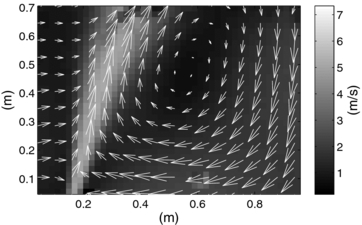
Figure 3. Ensemble averaged mean flow field (FoV: 0.9 m × 0.7 m) obtained from 1000 instantaneous LF-PIV realizations. Color contours represent velocity magnitude. Velocity vectors represent local mean velocity vector. Note: for the above measurements, velocity vectors are obtained every 20 mm within the measurement plane, however, to enable visualization vectors spaced every 60 mm are shown.
Download figure:
Standard image
Figure 4. Normalized standard deviation of velocity measured with respect to local mean measured using LF-PIV. Contours represent normalized standard deviation while vectors present local mean velocity. It is clear that the shear layers at the edge of the jet from the blower generate a significant amount of turbulence. Note: for the above measurements, velocity vectors are obtained every 20 mm within the measurement plane, however, to enable visualization vectors spaced every 60 mm are shown.
Download figure:
Standard imageSF-PIV measurements were also obtained on the same flow to allow for comparison studies. Three distinct sets of SF-PIV measurements were obtained. The measurements SF-PIV1 were obtained using Expancel particles at the region close to the edge of the jet having a measurement FoV: 0.07 m × 0.095 m. For SF-PIV1, an interrogation spot size of 128 × 128 pixels was selected with 50% overlap to yield a velocity vector spacing of ∼4 mm. Comparison between LF-PIV and SF-PIV1 measurements allowed for investigating the effect of increase in the FoV on the accuracy of measurements. The measurements SF-PIV2 and SF-PIV3 were obtained at a randomly chosen area (different from SF-PIV1) using Expancel and fog particles, respectively. The FoV for these measurements was restricted to 1.8 cm × 2.4 cm to avoid uncertainties due to a large FoV and exclusively compare the effect of using different particles on measurement accuracy. Table 2 summarizes the uncertainty and dynamic ratios of LF-PIV, SF-PIV1, SF-PIV2 and SF-PIV3. The estimates are for a 2 MP camera. The DLSR is estimated from equation (2) for Nx equal to 1600 pixels.
Table 2. Measurement uncertainty and dynamic ratios of LF PIV and SF PIV measurements obtained using a 2 MP camera.
| Measurement type | Image resolution (μm/pixel) | Time delay Δt (μs) | Uncertainty (m s−1) | DLSR | DVR |
|---|---|---|---|---|---|
| LF-PIV | 625 | 1500 | 0.04 | 50 | 160 |
| SF-PIV1 | 59 | 250 | 0.02 | 25 | 320 |
| SF-PIV2 | 15 | 150 | 0.01 | 25 | 320 |
| SF-PIV3 | 15 | 150 | 0.01 | 25 | 320 |
4.2. Comparison between SF-PIV2 and SF-PIV3
It was discussed in section 3.4 that the flow tracking ability of the particles improves with decrease in the particle density and size. The Expancel particles used as tracers to obtain LF-PIV measurements are considerably larger (80–100 μm) compared to typically used fog particles (1–10 μm). The large size of these particles is desirable to improve the particle image intensity. However, the flow tracking ability of the Expancel particles is deteriorated due to their large size. The low density of these particles does not deteriorate the flow tracking ability as much as it would have with similar sized olive oil droplets. As pointed out in section 3.4, the slip in velocity for Expancel particles is less than 0.45% for accelerations reaching  . Since slip velocity of olive oil particles is much lower (0.002%) and assuming that fog particles have similar flow tracking characteristics to olive oil droplets, it is expected that there should be a minor difference (ideally negligible) between SF-PIV2 and SF-PIV3 measurements.
Figure 5 shows mean velocity vectors and contours obtained using Expancel and fog particles averaged over 2500 realizations. The mean velocities measured using both methods are clearly in qualitative agreement. The mean velocities averaged over the plane of SF-PIV2 and SF-PIV3 measurements are 1.21 and 1.16 m s−1, respectively. The uncertainty for both measurements is 0.01 m s−1. Figure 6 shows contour plots of % difference in the statistics obtained using SF-PIV2 and SF-PIV 3 measurements.

Figure 5. Mean velocity vectors and contours obtained using Expancel (above) and fog particles (below) averaged over 2500 realizations. Note: for the above measurements, velocity vectors are obtained about every 1 mm within the measurement plane, however, to enable visualization vectors spaced every 2 mm are shown.
Download figure:
Standard image
Figure 6. Contour plot showing difference in mean velocity (above) and standard deviation (below) estimated using Expancel and fog particles.
Download figure:
Standard imageThe difference in mean velocity and normalized standard deviation averaged over the measurement plane is ∼4% and ∼8%, respectively. This difference in mean velocity is greater than predicted in section 3.4 for modest acceleration of  . The acceleration estimate is based on SF-PIV2 mean velocity (
 ) and an approximate distance of
  from the core of the vortex. The higher difference in velocity estimates can be attributed to several parameters that perhaps include enhanced out-of-plane motions and higher acceleration component not estimated by analysis in section 3.4 due to high velocity variation, or due to variation under experimental conditions (fan velocity etc) that may occur over the course of obtaining two separate sets of 2500 realizations (SF-PIV2 and SF-PIV3). Nevertheless, the difference in the velocity estimates points out the importance of characterizing the uncertainty of measurements obtained using non-standard tracer particles. In this case, the uncertainty in measurements due to the usage of Expancel particles is ∼4%, which is greater than the standard estimate of PIV uncertainty of <1% as shown in table 2 (uncertainty of
  for planar averaged mean velocity of
  ).
).
4.3. Comparison between LF-PIV and SF-PIV1
It is well known that each PIV measurement is an average of the velocity over the interrogation region. In the case of LF-PIV, this interrogation region (in the measurement space) is significantly larger. Therefore, effects of averaging over gradients in the flow become important. This effect can be studied by performing PIV measurements at multiple scales. To investigate this effect, both LF-PIV and SF-PIV1 measurements were performed on the same apparatus. Further, particle agglomeration might increase the particle diameters and result in increased particle slip. Since agglomerated particles scatter more light, bias errors are introduced in the measurement. These errors can also be investigated by a comparison of statistics from LF-PIV and SF-PIV1 measurements.
Figure 7 shows a comparison of the mean velocity vector field obtained by averaging 1000 instantaneous measurements using both LF-PIV and SF-PIV1 measurement methods. The SF-PIV1 measurements were obtained for a region where the flow field has a significant variation in direction and magnitude to maximize the deviation between LF-PIV and SF-PIV1, if any. The qualitative agreement seen in figure 7 is further investigated by plotting line outs of the mean horizontal and velocity fields at different vertical locations.

Figure 7. LF-PIV mean velocity field superimposed upon an SF-PIV mean velocity field. A magnified view of the vector field (above) is shown (below). Note: for the magnified view SF-PIV vectors spaced around every 7 mm are shown.
Download figure:
Standard imageFigure 8 plots profiles of U (mean horizontal) and V (mean vertical) velocity magnitudes comparing averaged LF-PIV and SF-PIV1 measurements at the overlapping measurement regions. For a wide range of velocities, the LF-PIV and SF-PIV1 measurements agree to within 1% of one another. The largest deviations are found near the edge of the jet from the blower. Figure 9 plots the average magnitude and standard deviation of the LF-PIV and SF-PIV1 velocities. Despite the high fluctuations, and the gradients, an average error of less than 8% is measured in the turbulence statistics. Thus, the bias errors due to agglomerated particles and gradients for the present flow are found to be small. Further, due to particle image diameter being close to 1 pixel, pixel-locking may be an issue (Christensen 2004), limiting the ability of LF-PIV to accurately predict sub-pixel displacements. To remedy the situation, the interframe-time delays may be set such that displacements are much greater than 1 pixel. Further, use of corrective algorithms such as described in Chen and Katz (2005), Gui and Werely (2002) or by slightly defocusing the particle images to increase their image size as described in Overmars et al (2010) could be used to reduce pixel-locking.
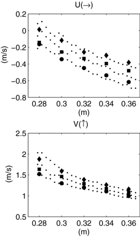
Figure 8. Profile of U (→) and V (↑) velocity magnitudes comparing averaged LFPIV and SF-PIV1 measurements at the overlapping measurement areas. The LF-PIV measurements are represented by solid shape markers and the SF-PIV1 measurements are represented by dots.
Download figure:
Standard image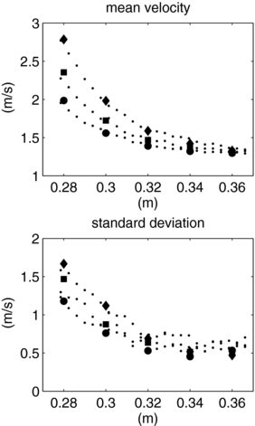
Figure 9. Profiles of mean magnitude of velocity and standard deviation comparing LF-PIV and SF-PIV1 measurements at the overlapping measurement areas. The LF-PIV measurements are represented by solid shape markers and the SF-PIV1 measurements are represented by dots.
Download figure:
Standard image4.4. Field of view enhancement
The FoV limitations imposed by the current apparatus were investigated by increasing the FoV beyond the previously obtained 0.75 m × 1 m. This increase in the FoV was obtained by using a shorter focal length lens (35 mm) on a 11 MP camera with a stand-off distance of 5 m. Increase in the FoV can be also obtained by increasing the stand-off distance for the 2 MP camera (60 mm lens) to about 5.4 m (not shown here). In both cases, the image resolution is approximately 1 mm per pixel to yield an FoV of 1.2 m × 1.6 m for the 2 MP camera or 2.8 m × 4.3 m for the 11 MP camera, respectively. Figure 10 plots the velocity field measured at FoV: 2.8 m × 4.3 m. The data yield in this case was restricted by the dimensions of the box in which the cross flow fan and the particles were enclosed. The test box was moved to various locations (left, center and right) within the camera FoV. At each location, the mean vector field was obtained by averaging over 1000 realizations. The velocity vectors were estimated using a similar image analysis technique to that used before. The FoV was divided into interrogation spots of size 64 pixels × 64 pixels with 50% overlap. The large-scale vortical structure created by the cross flow fan can be clearly observed in measurements made at various locations. There appears to be a minimal effect of variation in light sheet intensity on the data yield for measurements made at various locations within the FoV. Figure 10 also shows the relative dimensions of the SF-PIV1 FoV. Clearly, a significant enhancement of the FoV is possible due to the usage of larger size Expancel particles and appropriate modifications in the hardware.

Figure 10. Mean velocity vector field obtained using a 11 MP camera and 35 mm lens (FoV of 2.8 m×4.3 m). Vector fields were obtained by moving the test section to three different locations within the FoV. The smaller shaded rectangle shows the relative size of SF-PIV1 FoV. Note: for the above measurements, velocity vectors are obtained about every 32 mm within the measurement plane, however, to enable visualization vectors spaced approximately every 96 mm are shown.
Download figure:
Standard image5. Conclusions
Successful measurements of large flow fields using large field of view particle image velocimetry (LF-PIV) technique was demonstrated in a laboratory-scale confined vortex apparatus. Measurements over an area of 0.75 m × 1.0 m were achieved using a 2 MP camera that imaged side-scattered light from the particles. Although an even larger illuminated field of view (FoV) of 2.8 m × 4.3 m was achieved using a 11 MP camera, a sufficiently large flow was not available to test this FoV. The use of large sized, low-density Expancel particles to track the flow allowed a significantly large stand-off distance between the measurement plane and the camera. Despite the substantial increase in the time constant for the Expancel particles when compared to olive oil droplets (or fog particles), a slip velocity of less than 1.2% was estimated even for accelerations of 1000  , thus proving the efficacy of Expancel particles for LF-PIV measurements. However, it is recommended to conduct a comparison study similar to that in section 4.2 to quantify the uncertainty of LF-PIV measurements obtained using non-conventional tracer particles (e.g. Expancel particles). The error in measurements could arise due to parameters such as enhanced out-of-plane motions or higher acceleration components not estimated by analysis in section 3.4 due to high turbulence intensity of the flow. The errors may also be caused by pixel-lock issue due to the particle image size being 1 pixel caused by the low magnification inevitable for LF-PIV imaging. Further, bias errors due to particle agglomeration and flow field curvature were shown to be negligible (less than 1%) by comparing mean and turbulence velocity statistics from LF-PIV and SF-PIV experiments. Key scaling issues relevant for the successful design of LF-PIV diagnostics were presented to guide the design of future LF-PIV experiments. Based on these calculations, the LF-PIV appears to be a promising diagnostic for the measurement of large-scale flow fields, such as flows around wind turbines and the wall-region of the planetary boundary layer.
Acknowledgments
The support of Department of Energy's Energy Efficiency and Renewable Energy office through Grant EB2501030 and LANL's Laboratory Directed Research and Development Office through Grant 20100040DR are gratefully acknowledged. The authors thank Professor Ronald J Adrian for his advice and encouragement during the conduct of this research. The authors acknowledge constant support and co-operation of Dr William T Buttler and Dr Curtt Ammerman.