


Abstract
With x-ray computed tomography (CT) it is possible to evaluate the dimensions of an object's internal and external features non-destructively. Dimensional measurements evaluated via x-ray CT require the object's surfaces first be estimated; this work is concerned with evaluating the uncertainty of this surface estimate and how it impacts the uncertainty of fitted geometric features. The measurement uncertainty due to surface determination is evaluated through the use of a discrete ramp edge model and a Monte Carlo simulation. Based on the results of the Monte Carlo simulation the uncertainty structure of a coordinate set is estimated, allowing individual coordinate uncertainties to be propagated through the geometry fit to the final measurement result. The developed methodology enables the uncertainty due to surface determination to be evaluated for a given measurement task; the method is demonstrated for both measured and simulated data.
Export citation and abstract BibTeX RIS
1. Introduction
Dimensional metrology plays a central role in manufacturing industries for the purpose of quality assurance. Although a wide variety of inspection tasks can be performed with conventional measurement instruments, such as coordinate measuring machines (CMMs) and surface profilers, these instruments are not able to measure internal or complex external features due to limitations imposed by feature accessibility. On the other hand, x-ray computed tomography (CT) is able to resolve both the internal and external structure of an object in a single scan, hence providing a non-destructive solution to this measurement problem. There are many advantages in using x-ray CT for dimensional metrology, such as fast scan time, non-contact measurement and micron-level spatial resolution, however, the technique is not without its shortcomings. There are numerous factors that can influence dimensional measurements evaluated via x-ray CT, these include, but are not limited to, the geometric alignment of the instrument's hardware [1], user defined scan parameters, the composition, orientation and size of the object being scanned, the algorithm used to reconstruct the object from its radiographic projections and the surface determination method [2], which ultimately defines the surface from which dimensions are evaluated; this work is concerned with the latter.
The objective of surface determination is to identify transitions between pixels, or voxels, representing different materials, i.e. the object surfaces, both internal and external. This task is essentially 2D or 3D edge detection, but is referred to here as surface determination. Surface determination generates a set of discrete surface coordinates to which geometric primitives are fitted and dimensional information evaluated. As a consequence, the uncertainty of the surface coordinates directly influences the uncertainty of the fitted geometric feature and hence the measurement result. Figure 1 illustrates this idea and shows the search for the edges of a circle: each edge point has coordinates xi, yi with associated uncertainties σxi, σyi. A circle is fitted to the coordinates by the least-squares method, hence the uncertainty of the coordinates directly impact the radius uncertainty σr. This work is concerned with first estimating coordinate uncertainties, and then propagating them through a least-squares fit to the final measurement result.
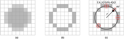
Figure 1. Illustration of the measurement uncertainty due to surface determination. (a) CT image of an object with a circular cross-section. (b) Detected edge of the circle. (c) A circle fitted to the sub-pixel edge coordinates.
Download figure:
Standard image High-resolution imageThe contributions of this work are twofold: firstly, based on a discrete ramp edge model and a Monte Carlo simulation, a method for estimating the uncertainty of an edge's position is developed (sections 2.2, 2.3 and 3.1). Secondly, using the results of the Monte Carlo simulation, a method for estimating the uncertainty due to surface determination is developed (section 3.3).
2. Methodology
The key idea of this paper is to use a Canny type edge detector [3] to repeatedly estimate the localisation error of a synthetic ramp edge, where localisation error is the difference between the actual position of an edge and that estimated by the edge detector. By repeatedly estimating the localisation error in a Monte Carlo simulation the standard deviation of the error is evaluated and forms an estimate of the uncertainty of the localisation error. The results of the Monte Carlo simulation act as a lookup table (LUT) which is used to estimate the uncertainty of surface points evaluated from a given CT data-set. The uncertainties for all surface points are then propagated through a least-squares fit to the final measurement result. To demonstrate the method, surfaces are estimated from measured and simulated CT images of an aluminium workpiece.
2.1. Measured and simulated CT data
The proposed method for evaluating the uncertainty due to surface determination is evaluated for measured and simulated CT data of a workpiece with various cross-sectional geometries, see figure 2. The dimensional features of the workpiece include both internal and external radii, of which reference measurements are made on a Zeiss PRISMO tactile CMM. The reference measurement uncertainty is evaluated using the substitution method as per ISO15530-3 [4] and a setting ring gauge is used as the measurement standard. The reference measurements are given in table 1.

Figure 2. Workpiece and CT data for testing the proposed method for evaluating the uncertainty due to surface determination. (a) Multi cross-section aluminium workpiece. (b) Technical drawing of the multi cross-section aluminium workpiece, all dimensions in mm. (c) Simulated CT image. (d) Measured CT image.
Download figure:
Standard image High-resolution imageTable 1. Tactile CMM measurements of the multi cross-section workpiece in figure 2.
| Inner diameter | |
|---|---|
| Mean (mm) | 22.631 |
| Uncertainty (mm) (K = 2) | 0.002 |
The multi cross-section workpiece is scanned with an YXLON Y.FOX CT system. The CT system features a 160 kV x-ray source with a tungsten transmission target. The detector is a Varian PaxScan, with 1480 × 1848 pixels and a pixel size of 0.127 mm. 720 projections are acquired with the x-ray source voltage and current set to 160 kV and 17.5 µA respectively.
Simulated projections of the workpiece are generated using in-house developed software. The simulation considers the geometric un-sharpness due to the finite size of both the x-ray focal spot and the detector pixels. Additionally, the polychromatic x-ray spectrum and energy dependence of the detector are considered alongside noise in the projections.
Both measured and simulated data sets are reconstructed into 10243 CT volumes with VGStudio MAX 2.1. The measured data is aligned using a '3-2-1' procedure and CT images extracted in the same planes as the reference measurements, see figure 2.
2.2. Ramp edge model
The edges of objects in CT data are not ideal step edges, but ramp edges, this is due to the point spread function (PSF) that arises from data acquisition and reconstruction [5]. We adopt a discrete 2D ramp edge model based on the work of Rockett [6], who in turn based the model on that of Lyvers & Mitchell [7]. A step edge is parameterised in terms of its sub-pixel displacement from the origin t, its orientation θ and contrast-to-noise ratio (CNR). The intensity of each pixel is calculated based on the relative area of high and low intensity regions, see figure 3.

Figure 3. Ramp edge model used in the Monte Carlo simulation. (a) Illustration of Rockett's step edge model. (b) Exemplary edge generated in the Monte Carlo simulation. CNR = 7.1, σ of PSF = 6.1 pix (see figure 4), t = 0.1, θ = 45°.
Download figure:
Standard image High-resolution imageTo approximate a ramp edge the step edge is convolved with the PSF of the imaging system. An imaging system's response to an edge is the edge response function (ERF), the first derivative of which is an approximation of the line spread function (LSF) which in turn is roughly equivalent to a profile taken perpendicular to a circularly symmetric 2D PSF [8]. ASTM E1695-95 [9] provides instruction on evaluating the ERF and LSF from CT data; the procedure described in the standard is adopted here. Figures 4(a) and (b) show the ERF and LSF evaluated from the inner edge of the CT image shown figure 2(c). A Gaussian function is fitted to the LSF to estimate its spread; due to the rotational symmetry of the Gaussian the PSF is estimated by simply extending the 1D Gaussian to 2D.
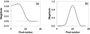
Figure 4. ERF and LSF evaluated from the inner edge of the CT image shown in figure 2(c). (a) ERF, (b) LSF, standard deviation of fitted Gaussian = 6.1 pixels.
Download figure:
Standard image High-resolution imageAfter convolution of the step edge with the PSF the ramp edge is superimposed with white Gaussian noise; the standard deviation of which is defined by evaluating the CNR for the inner edge of the CT image in figure 2(c). The noised ramp edge is then passed to the surface determination algorithm.
The sub-pixel displacement of the edge is varied from 0.1 to 0.4 pixels and the edge orientation from 0 to 45°. The edge symmetry implies all results are periodic for intervals of 45°. For each set of edge parameters 1000 repeated simulations are performed and the mean and standard deviation of the localisation error evaluated, a new noise waveform is generated for each repeat thus forming the Monte Carlo method.
2.3. Surface determination method
The surface determination method is based on the Canny algorithm [3]. The image is first convolved with a 5 × 5 Gaussian filter and the image gradient calculated using a 1 × 5 derivative of Gaussian filter (DOG) applied in the x and y directions. The standard deviation of the Gaussian and DOG filters are both 5/6 pixels. Local maxima are identified via non-maximum suppression (NMS), followed by hysteresis thresholding of the gradient magnitude. Hysteresis thresholding is not necessary when evaluating the edge model since the edge is correctly identified by NMS. However, for the CT data-sets evaluated in section 3.3 hysteresis thresholding is required. The two thresholds are automatically defined by fitting a Rayleigh distribution to a smoothed histogram of the gradient magnitude after NMS. The thresholds are then a function of the distribution peak, as evaluated by Voorhees [10]. Finally, second order polynomials are fitted to the gradient magnitude normal to the edge; the turning point of which gives the sub-pixel surface position.
3. Results
3.1. Results of the Monte Carlo simulation
Figure 5 shows how the localisation error varies as a function of edge displacement t and edge orientation θ in the absence of noise. The localisation error increases with both t and θ and reaches a maximum for t = 0.4 and θ = 35–40°. The localisation error is very small, at worst it is approximately 1/25th of a pixel, however, in the presence of noise the localisation error becomes much larger. Figure 6 shows how the mean localisation error varies as a function of t and θ in the presence of noise. For values of t that are not equal to 0 a bias is observed and the localisation error becomes independent of θ. This is likely due to the combined effect of the PSF and noise blurring the edge into the neighbouring pixels; in CT this is known as the partial fill artefact which arises due to the finite spatial resolution of the imaging system. Mikulastik et al [11] showed that using polynomials for the sub-pixel estimate can introduce a bias in the estimated edge position; the bias seen in figure 6 is in line with the calculations of Mikulastik et al.

Figure 5. Localisation error for noiseless ramp edges with various sub-pixel displacements and orientations.
Download figure:
Standard image High-resolution image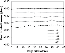
Figure 6. Mean localisation error for 1000 repeated simulations of noisy ramp edges with various sub-pixel displacements and orientations.
Download figure:
Standard image High-resolution imageFor each run of the Monte Carlo simulation the x and y coordinates of the edge position are estimated, figure 7 shows how the standard deviation of these xy coordinates varies as a function of t and θ. It is found the coordinate uncertainties act in opposition and converge at 45°. Figure 7 also shows for θ = 0° (a vertical edge) the y coordinate uncertainty is minimum whilst the x coordinate uncertainty is a maximum; i.e. the coordinate uncertainty is maximum when perpendicular to the edge and minimum when parallel to the edge. This explains why both the x and y coordinate uncertainties converge at θ = 45°.

Figure 7. Standard deviation of x and y coordinates versus edge orientation.
Download figure:
Standard image High-resolution image3.2. Discussion of Monte Carlo simulation results
Figure 7 shows the standard deviation of the x and y coordinates vary with both edge orientation and sub-pixel displacement. This is an important result because least-squares fitting is based on the assumption the standard deviation of coordinate error is constant; this property is termed homoscedasticity [12]. Thus for geometric features with varying edge orientation, such as circles, spheres and ellipses this assumption of homoscedasticity is violated. If, however, the uncertainty structure of the coordinate set is known then the weighted least-squares method can be used, whereby each coordinate is weighted by the inverse of its variance.
Figure 7 is particularly useful as it enables the uncertainty of an edge's position to be estimated for a given t and θ. Thus if we know t and θ for each surface point in a CT data-set we can estimate the respective coordinate uncertainties. θ is estimated directly by the surface determination algorithm. Unfortunately t can't be estimated as the actual edge position is unknown. Instead we use the maximum envelope of figure 7; this is shown in figure 8. With figure 8 the uncertainty of an edge's position can be estimated with only knowledge of its orientation θ. Figure 8 forms a LUT that is used in the next section to estimate the uncertainty of surface coordinates from measured and simulated CT data. The individual coordinate uncertainties are then propagated through a least-squares fit to the final measurement result.

Figure 8. Maximum envelope of figure 7.
Download figure:
Standard image High-resolution image
3.3. Estimating the measurement uncertainty due to surface determination
The results of the Monte Carlo simulation are used in this section to estimate the measurement uncertainty due to surface determination for the inner radius of the multi cross-section aluminium workpiece; both measured and simulated data are considered. The graphs in section 3.1 correspond to the simulated CT image in figure 2(c), thus these results are used as a worked example.
Applying the surface determination algorithm to the CT image in figure 2(c) yields a vector of surface coordinates xi and yi, alongside a vector of edge directions θi, for i = 1 to m. With the aid of figure 8 the uncertainty of each coordinate xi, yi, denoted σxi and σyi respectively, is estimated. We fit a circle to the coordinates xi and yi using weighted least-squares so as to consider the uncertainty of each point. Weighted least-squares minimises

where wi is a vector of weights. The weights are a function of the standard deviation of the localisation error σi such that high-quality data points influence the fit more than low-quality data points:

For the linear least-squares circle-fit,  in equation (1) is written:

where

where xc, yc represent the centre coordinates of the circle and r its radius. Equation (3) is therefore rewritten:

Expanding:

let

which simplifies equation (6) to

Forming the equations in matrix notation:
The u that minimises F is the solution of the linear system of equations

The radius estimate is recovered by

With estimates of xc, yc and r the uncertainty of the fitted radius is evaluated via a second Monte Carlo simulation. Pseudo-random numbers are added to each surface coordinate xi, yi and a circle fitted to the coordinate set. This is repeated 100 000 times in order to evaluate the standard deviation of the radius estimate. The standard deviations of the pseudo-random numbers added to each coordinate are defined by σxi and σyi as evaluated via figure 8. The coordinate set for each run of the Monte Carlo simulation is therefore
where n is a random number drawn from the standard normal distribution.
The results of the weighted least-squares circle-fit for the CT image in figure 2(c) are given in table 2 alongside the uncertainty of the radius evaluated via the second Monte Carlo simulation. The results show the radius is measured with sub-pixel uncertainty. Furthermore, the radius uncertainty is significantly lower than the individual coordinate uncertainties shown in figure 8. Such a low uncertainty is unexpected; however; the result can be rationalised based on the following considerations: firstly, the number of surface points used in the geometric fit is large (m = 987); if m is large then the radius uncertainty will be small. Secondly, for the considered measurement task, the dimension of interest r is large compared to the pixel size; r is nominally 22.6 mm whilst the pixel size is 49 µm. Based on this reasoning, the uncertainty due to surface determination will be larger for dimensional features that fill only a portion of a CT image and for features fitted to few surface points.
Table 2. Measurement uncertainty due to surface determination for simulated CT data.
| Pixel size = 49 µm | Radius (pixels) | Radius (mm) | Uncertainty due to surface determination (pixels) | Uncertainty due to surface determination (µm) |
|---|---|---|---|---|
| Figure 2(c) | 230.324 | 11.286 | 0.0066 | 0.32 |
To verify the result presented in table 2 we make use of the CT simulation tool described in section 2.1; 20 CT data-sets of the cross-section shown in figure 2(c) are generated, each with a different noise waveform. For each data-set surface determination is performed and the radius evaluated; the standard deviation of the repeated radius estimation is calculated and found to be 0.0066 pixels. This is in agreement with the result presented in table 2 and thus verifies our method.
Finally, the developed method is applied to the measured CT image shown in figure 2(d). The steps taken are summarised as follows:
- The PSF of the inner edge is evaluated. Fitting a Gaussian function to the PSF yields a standard deviation of 7.4 pixels.
- The CNR of the inner edge is evaluated and found to be 7.3.
- The above PSF and CNR are input to the Monte Carlo simulation so as to generate a LUT for σx and σy.
- Surface determination is performed giving the surface coordinates xi and yi.
- Using the LUT σxi and σyi are evaluated.
- The surface coordinates xi, yi and their respective uncertainties σxi and σyi are input to the second Monte Carlo simulation to estimate uncertainty of the radius due to surface determination.
The results for estimating the uncertainty due to surface determination for the measured CT data are given in table 3. Comparing the results in tables 2 and 3 shows the measurement uncertainty due to surface determination is larger for the measured data than the simulated data. This result is predominantly due to fewer surface points being used when fitting the least-squares circle. For the measured data m = 121 whereas for the simulated data m = 987. Fewer surface points are used because the measured data suffers from additional artefacts, such as ring artefacts, which are caused by defective detector pixels. As a consequence, surface points that deviate from the fitted geometric form by more than one pixel are omitted from the least-squares fit. In general, omitting outliers in this way improves the fit but reduces the number of fit points, which, as can be seen from the results, increases the measurement uncertainty due to surface determination.
Table 3. Measurement uncertainty due to surface determination for measured CT data.
| Pixel size = 49 µm | Radius (pixels) | Radius (mm) | Uncertainty due to surface determination (pixels) | Uncertainty due to surface determination (µm) |
|---|---|---|---|---|
| Figure 2(d) | 230.382 | 11.289 | 0.025 | 1.22 |
4. Discussion
The localisation error of different edge detection algorithms have been studied by a number of authors [6, 11, 13–16]. However, these have either been mathematical analyses or only considered step edges. Furthermore, no exclusive treatment has been given to the uncertainty of localisation error in the field of x-ray CT for dimensional metrology.
Surface determination defines the coordinate set from which the dimensions of an object are evaluated and thus influences the accuracy and uncertainty of dimensional measurements. It has been shown that with knowledge of the edge response function (ERF) and contrast-to-noise ratio (CNR) it is possible to estimate the measurement uncertainty due to surface determination. The method presented here need not be limited by knowledge of the system ERF, exemplary edge profiles can be used instead. For objects with non-axially symmetric cross-sections we suggest using 'worst case' edge profiles so as to overestimate the coordinate uncertainty.
The input parameters of our method are the PSF and CNR of the considered data-set. Thus any factors that influence the PSF and CNR of the data-set will influence the measurement uncertainty due to surface determination. A non-exhaustive list of factors that influence the PSF and CNR include: x-ray source settings, detector settings, scattered radiation, beam hardening, x-ray focal spot drift, rotational axis run-out, thermal expansion, vibration and reconstruction algorithm. Therefore, our method considers the entire measurement workflow. The only obvious limitation is the 2D implementation, however, extending the method to 3D should be relatively straightforward and will be considered in future work.
The uncertainty of edge localisation has been shown to vary with both edge orientation and sub-pixel displacement, thus violating the assumption of homoscedasticity for least-squares fitting. However, since it is possible to evaluate the uncertainty structure of the coordinate set this information can readily be incorporated in the weighted least-squares method. Both Forbes et al [17] and Cox et al [18] give details of how coordinate uncertainty can be further used in least-squares fitting.
The measurement uncertainty due to surface determination was evaluated using Monte Carlo simulations. This method is well suited for incorporating in existing CT uncertainty budgets that consider additional influencing factors, such as those evaluated by Hiller et al [19] and Camignato et al [20].
5. Conclusions
The uncertainty of edge localisation has been shown to vary with edge orientation and sub-pixel displacement. This observation violates the assumption of homoscedasticity in least-squares fitting. With a ramp edge model and a Monte Carlo simulation the uncertainty structure of a coordinate set has been estimated. The individual coordinate uncertainties have been propagated through a least-squares fit to the final measurement result. This methodology is suitable for comparing the performance of surface determination algorithms, alongside evaluating the measurement uncertainty due to surface determination.