


Abstract
Enclosed flow apparatuses with negligible mean flow are emerging as alternatives to wind tunnels for laboratory studies of homogeneous and isotropic turbulence (HIT) with or without aerosol particles, especially in experimental validation of Direct Numerical Simulation (DNS). It is desired that these flow apparatuses generate HIT at high Taylor-microscale Reynolds numbers ( ) and enable accurate measurement of turbulence parameters including kinetic energy dissipation rate and thereby
  . We have designed an enclosed, fan-driven, highly symmetric truncated-icosahedron 'soccer ball' airflow apparatus that enables particle imaging velocimetry (PIV) and other whole-field flow measurement techniques. To minimize gravity effect on inertial particles and improve isotropy, we chose fans instead of synthetic jets as flow actuators. We developed explicit relations between
  and physical as well as operational parameters of enclosed HIT chambers. To experimentally characterize turbulence in this near-zero-mean flow chamber, we devised a new two-scale PIV approach utilizing two independent PIV systems to obtain both high resolution and large field of view. Velocity measurement results show that turbulence in the apparatus achieved high homogeneity and isotropy in a large central region (48 mm diameter) of the chamber. From PIV-measured velocity fields, we obtained turbulence dissipation rates and thereby
  by using the second-order velocity structure function. A maximum
  of 384 was achieved. Furthermore, experiments confirmed that the root mean square (RMS) velocity increases linearly with fan speed, and
  increases with the square root of fan speed. Characterizing turbulence in such apparatus paves the way for further investigation of particle dynamics in particle-laden homogeneous and isotropic turbulence.
Export citation and abstract BibTeX RIS
List of abbreviations and mathematical symbols
| HIT | Homogeneous and isotropic turbulence |
| PIV | Particle image velocimetry |
| DNS | Direct numerical simulation |
| RMS | Root mean square |
| CCD | Charge coupled device |
| SNR | Signal-to-noise ratio |
 and and  | Consolidated coefficient in equation (10) |
 and and  | Consolidated coefficient in equation (12) |
 | Constant, from second-order structure function |
 | Constant, from second-order structure function assuming infinite Reynolds number |
 | Actuator outlet diameter |
 | Longitudinal velocity structure function |
 | Second-order longitudinal velocity structure function |
 | Fan rotational speed |
 | Froude number |
 | Integral length scale |
 | Number of actuators |
 | Order of the structure function |
 | Fluid mean velocity near the actuator outlet |
 | Chamber radius |
 | Integral scale Reynolds number |
 | Taylor microscale Reynolds number |
 | To be estimated taylor microscale Reynolds number |
 | Reference Taylor microscale Reynolds number |
 | RMS velocity fluctuation in horizontal direction in the HIT chamber |
 | RMS velocity fluctuation in vertical direction in the HIT chamber |
 | Mean velocity in horizontal direction in the HIT chamber |
 | Mean velocity in vertical direction in the HIT chamber |
 | Turbulence strength at the origin point |
 | Turbulence strength at the local measurement point |
 | Turbulence strength |
 | Isotropy index |
 | Homogeneity index |
 | Kinematic viscosity of fluid |
 | Taylor microscale |
 | Turbulent kinetic energy dissipation rate |
 | Distance of two fluid elements |
 | Separation vector of two fluid elements |
 | Unit vector in the direction of separation of the two fluid elements |
 | Turbulence fluctuating velocity |
 | Eddy turnover time |
 | Turbulent kinetic energy |
 | Large Eddy length scale |
 | Large Eddy time scale |
 | Kolmogorov length scale |
 | Kolmogorov time scale |
 | Kolmogorov velocity scale |
 | Fan motor speed of operation |
1. Introduction
Generation of homogeneous and isotropic turbulence (HIT) in laboratories is important for a wide range of applications of turbulent flow including particle-laden flows. Statistical theories of turbulence are based on the homogeneous and isotropic assumption [1, 2], but direct testing of many theories is difficult, since it has been challenging to realize homogeneous and isotropic turbulence in the laboratories [3]. With the advent of supercomputing, direct numerical simulation (DNS) has become a major vehicle to explore particle dynamics in turbulent flows [4–6]. However, simulation results require validation, which again hinges on our ability to obtain relevant experimental data.
Traditionally, homogeneous and isotropic turbulence are generated by passive or active grids in wind tunnels. It is difficult to introduce aerosol particles in a wind tunnel homogeneously or to recover the particles for re-use. Moreover, flow in a wind tunnel has a large mean velocity. This is not conducive for investigating Lagrangian properties of particles, which require particle tracking [7].
To overcome these limitations, enclosed flow chambers with negligible mean flow are emerging as alternatives to wind tunnels. This class of flow facilities typically generates HIT in the center region through symmetrically distributed actuators along multiple axes [7]. They enjoy several advantages over wind tunnels: smaller sizes, lower power consumption, convenient particle recycling, significantly reduced expenses of experimentation, and ease of measurement, especially for Lagrangian properties. Hwang and Eaton [3] developed the first apparatus with multiple synthetic jet actuators as forcing mechanism. They placed 8 synthetic jets (a loudspeaker attached to a nozzle) at the 8 corners of a cubic box, one at each vertex facing toward the center, and generated HIT with negligible mean flow in the center. They used this new apparatus to study both stationary and decaying turbulence. In a similar cubic air chamber, Lu et al [8] measured Lagrangian particle trajectories. Goepfert et al [9] created an open-walled octahedron system with 8 centrally located synthetic jets opposing one another to study evaporating droplets in the presence of turbulence. Increasing the number of axes of symmetry, Chang et al [10] and Bewley et al [11] approximated a sphere by using a truncated icosahedron chamber with 32 synthetic jets distributed spherically about the center. By modulating the relative intensity of the jets, they were able to create isotropic turbulence as well as introduce various degrees of anisotropy. They used Laser Doppler Velocimetry (LDV) to study the influence of anisotropy on the inertial scales of turbulence.
With the primary objective of studying dynamics of inertial particles in HIT, our lab took a different approach to flow chamber design. In order to increase air agitation to reduce the relative influence of gravity on particles, de Jong et al [12] in our lab used fans instead of synthetic jets as actuators to force turbulent flow. We created a cubic air chamber with 8 fans at the vertexes, similar to the apparatus published by Birouk et al [13]. This apparatus enabled us to study inertial particle clustering and relative velocity in homogeneous and isotropic turbulent flow using Particle Imaging Velocimetry (PIV) and holographic PIV [6, 14, 15].
Up to now, few of existing enclosed turbulence chambers offer homogeneous and isotropic turbulence at high Reynolds numbers. Owing to the advancement of computing power, DNS of particle-laden turbulent flow are performed at increasingly higher Reynolds numbers, mostly under the homogeneous and isotropic assumption without including gravity [16, 17]. In order to validate DNS results, it is therefore desired that an experimental HIT apparatus provides high enough Reynolds numbers that are comparable to DNS, minimizes the gravity effect on particles, and accommodates whole-field flow measurement techniques including PIV.
To this end, we have designed, constructed and characterized an enclosed, fan-driven, highly symmetric 'soccer ball' airflow chamber that enables PIV as well as other whole-field flow measurement techniques, with a high Taylor-microscale Reynolds number  and a negligible effect from gravity. Modified from the turbulence chamber by Chang et al [10], our HIT 'soccer ball' airflow chamber uses fans instead of synthetic jets as actuators, as in de Jong et al (2009). Furthermore, our apparatus has built-in large windows to enable PIV measurement and holographic imaging. To meet the intrinsic challenge of acquiring accurate PIV data in a nearly zero-mean flow, we have developed a new two-scale PIV measurement technique to achieve both high spatial resolution and large flow field of view, and utilized cross-validation of two independent PIV measurements to improve the accuracy of turbulence characterization of the HIT flow apparatus.
2. Design and implementation of the enclosed HIT apparatus
For the purpose of studying particle-laden turbulence, a high-Reynolds-number HIT chamber should possess the following flow characteristics: nearly zero mean velocity (requiring the system to be highly symmetrical), minimal gravity effect (requiring high Froude number, important for studying particle dynamics), flow homogeneity and isotropy in a large region, and a high  . From a practical standpoint, the apparatus should also allow particles to be easily dispersed into the flow field and allow the particles and the carrying flow to be visualized and measured optically. These requirements call for careful selections of design parameters.
2.1. Geometrical symmetry
With a given physical space, a chamber that is nearly spherical has the highest degree of symmetry and the largest volume, and thereby is most advantageous for achieving high homogeneity, isotropy and  . However, a spherical chamber is difficult to construct. Chang et al [10] proposed a truncated icosahedron to approximate a sphere for use as an enclosed flow chamber. It has 20 hexagonal faces and 12 pentagonal faces for mounting hardware. This highly symmetrical shape, ideal for an enclosed chamber, was adopted in our chamber design. In principle, all 32 faces could be utilized for mounting flow actuators [10]. However, the hexagonal faces and pentagonal faces have different distances to the center of the truncated icosahedron. To mount actuators on a sphere without varying the length of the actuators, we decided to mount 20 identical actuators on the 20 hexagonal faces, which have equal distances to the center owing to the built-in symmetry of the icosahedron.
Our truncated icosahedron, or 'soccer-ball', chamber had a 1-meter outer diameter. The distances from the center of the solid to the centroids of the pentagonal and hexagonal faces are approximately 47.0 and 45.8 centimeters, respectively.
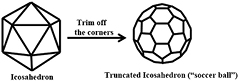
Figure 1. Geometry from icosahedron to truncated icosahedrons.
Download figure:
Standard image High-resolution image2.2. Actuators for generating turbulent flow
An enclosed HIT facility requires symmetrically distributing a number of actuators about the homogeneous and isotropic interrogation volume along multiple axes of symmetry. Both fan or 'continuous jet' [6, 12, 14] and loudspeaker attached to a nozzle or 'synthetic jet' [3, 9–11] have been used as flow actuators in HIT facilities.
We chose continuous jets over synthetic jets to minimize the gravity effect on particles to be studied. A synthetic jet uses a loudspeaker to draw in and push out air (which can be laden with particles) of a nozzle cavity through an orifice. A continuous jet uses a rotating fan to agitate air. Using multiple, symmetrically placed continuous jets, we can produce high mixing efficiency and turbulent kinetic energy dissipation rate, thereby achieving a high Froude number—the ratio of Kolmogorov-scale turbulence acceleration to gravitational acceleration. A high Froude number allows us to minimize the influence of gravity on particle dynamics.
Another reason fans are preferred over synthetic jets in our design is the need to avoid particle deposition in the corners of the nozzle. In synthetic jets, particles tend to be deposited and trapped around the oscillating diaphragm due to vortex generation near the jet orifice [18, 19]. When studying dynamics of particles of different Stokes numbers, it would be difficult to clean out trapped old particles from the synthetic jets. With fans, there are no flow cavities for particles to be deposited in. Moreover, loudspeakers employed in synthetic jets may generate variable standing-wave acoustic fields inside an enclosed chamber, and these sound fields could undermine the repeatability of the HIT facility.
To minimize disturbances to the flow and heating of the fluid within the chamber, motors can be mounted outside the chamber, and only the axes that drive the fans cross the hexagonal walls.
2.3. Flow homogeneity and isotropy
In an enclosed HIT apparatus, symmetrical flow forcing along more than 6 axes can produce turbulence with no preferred directions in the center [7, 10]. It is expected that turbulence in this region is not only homogeneous, but also isotropic. Furthermore, by virtue of the symmetrically placed multiple actuators, such a region has a nearly zero mean velocity.
In order to quantify the degree of homogeneity and isotropy, we define a homogeneity index  and an isotropy index
  [3, 10, 11]:
where  ) is the turbulence strength,
  and
and  are respectively the root-mean-square (RMS) velocity fluctuation in the horizontal and vertical directions at any point in the chamber, and the designations 'center' and 'local' refer to value at the origin point and a local measurement point in the chamber, respectively. In ideal homogeneous and isotropic turbulence,
  and
and  . However, in a real apparatus, system errors including imbalance and fluctuation of fans and environmental as well as measurement noise will cause
  and
and  to deviate from unity. Thus,
  and
and  have been frequently accepted [3, 12, 14]. Notably, Chang et al [10] achieved a homogeneity and isotropy region with
  and
and  fluctuations within 5% around 1. Since we would like the HIT apparatus to be useful for DNS validation with high reliability, we adopt the 5% requirement and define the 'homogeneous region' as a region in which the velocity fluctuations in all locations are within 5% of that at the center of the chamber, and the 'isotropic region' as a region where RMS velocity fluctuations in different directions are within 5% of each other. As such, a combination of
  and
and  qualifies for the homogeneous and isotropic region in our chamber.
2.4. Taylor microscale Reynolds number
The characteristic Reynolds number in homogeneous and isotropic turbulence is conventionally defined as  in terms of the Taylor microscale:
where  is the turbulence strength,
  is the viscosity of the flow, and
  is the Taylor microscale of turbulence. Finding the
  dependence on the physical parameters of the enclosed chamber is important for understanding, generating and controlling turbulence in enclosed HIT chambers. Therefore, in what follows we will develop a relationship between
  and chamber and actuator parameters.
Following Pope [2], we define large-eddy (or integral) length scale as
and integral-scale Reynolds number as
where the turbulent kinetic energy  . From equations (3)–(5) it follows that
or equivalently,
Based on energy conservation, we assume that the turbulent kinetic energy  at the center of an enclosed, symmetrically forced multiple-actuator HIT chamber is proportional to the kinetic energy provided from all the actuators or jets:

where  is the number of actuators and
  is the mean flow velocity generated by the actuators. Furthermore, we assume that the integral length scale
  is proportional to the chamber radius,

This is based on the consideration that in an enclosed turbulence system, the fluid continually recirculates inside a finite space, forming the largest flow structure by impinging at the center and then pushing back to the inlet of actuators (figure 2). Substituting equations (8) and (9) into equation (7) and consolidating coefficients into a facility constant  , we obtain the
  dependence on physical parameters of the chamber as:
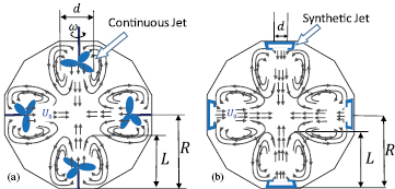
Figure 2. Sketch of flow structures and dimensions inside a zero-mean enclosed chamber. (a) A fan-driven chamber; (b) A loudspeaker-driven chamber.  is the mean flow velocity of a jet,
  is the diameter of jet,
  is the rotational speed of fan,
  is the integral length scale, and
  is the radius of the chamber.
Download figure:
Standard image High-resolution imageThis important relationship shows that  is proportional to the number of actuators
  to the power 1/4, the square root of jet velocity
  at the actuator exit, the square root of chamber radius
  and the square root of fluid viscosity
  . The jet velocity
  from an actuator depends on the power input and the energy conversion efficiency of the actuator.
The  relation in equation (10) is applicable to any type of actuators, including fans and synthetic jets (figures 2(a) and (b), respectively).
Next, when rotating fans are used as actuators (figure 2(a)), jet velocity  can be further determined by the flow volume per fan rotation
  , fan rotational speed
  , and fan diameter
  :
:
Substituting equation (11) into equation (10) and consolidating coefficients into a single coefficient  , we get an updated
  relation specifically for fan-driven HIT chambers:
Equation (12) illustrates the dependence of  on physical factors in a fan-driven HIT chamber, and was used in the process of designing our apparatus. To realize a desired
  , we could select the fan parameters (
 and
and  ), the motor speed of operation (
 ), and number (
 ) of fans and the kinematic viscosity (
 ) of the fluid. For any commercial fan, a rated CFM (cubic feet per minute) at a given fan speed
  is always given by the manufacturer. From the rated CFM, the flow volume per fan rotation
  can be obtained from dividing CFM by
  . The coefficient
  depends on the flow chamber.
To estimate  for our new 'soccer ball' chamber, we used our previous apparatus [12], which was fully characterized, as a reference chamber to eliminate the unknown coefficient C. From equation (12) we can take a ratio of the Reynolds number of the new chamber to be estimated,
 , to the Reynolds number of the reference chamber (denoted by 'prime'),
  :
:
Since both chambers use the same fluid—room air, we have  . Furthermore, we assume
  . Then
The reference chamber had  8 fans with
  11 cm, a maximum motor speed
  (fan rotational speed
  ), an equivalent radius of
  28.82 cm, and a maximum
  = 184. The fan had a rated
  at 3700 RPM. This yields
  per rotation. Plugging these numbers into equation (14) allows us to estimate the Taylor-scale Reynolds number for the new chamber,
  , under given design parameters.
For our new HIT chamber, our design goal was  400. We chose a robust motor (A.O. Smith 91 1/15 HP 115/230 Volt) with a maximum rotation speed of
  RPM (
RPM ( ). We adopted a plastic fan of diameter
  =16 cm (Dayton 5JLP3) with a rated
  at 3000 RPM. This yields
  per rotation. The new chamber had a radius
  and
and  =20 fans, as described in section 2.1. Plugging these values and those of the reference chamber into equation (14), we estimated the maximal
  in the new 'soccer ball' chamber to be
2.5. Working fluid and operating temperature
Air is usually preferred as the working fluid in the chamber. To change  via varying the fluid viscosity
  , either the working fluid or the operating temperature of the chamber [20] can be adjusted. Both numerical [21] and experimental [22, 23] studies have demonstrated that by choosing hexafluorides (
 ,
,  , and
, and  ), oxyfluorides (
 ,
,  ) or Freon-12 (
 ) as fluid in wind tunnels, the same
  can be obtained with lower power requirement. However, these gases are generally either toxic to the experimenter or environmentally hazardous, thus requiring a well-sealed chamber constructed with low permeability materials. We chose air as the working fluid without pressurizing the chamber for ease of operation.
Fluid viscosity can be sensitive to the operating temperature [24]. To maintain constant air viscosity during data acquisition, the facility should operate at a constant temperature, for which active cooling can be considered. In absence of active temperature regulation, sufficient time lapses should be allowed between experimental runs to avoid appreciable heating, allowing the chamber to operate near room temperature.
2.6. Optical access
Noninvasive diagnosis of the flow or the particle without disrupting flow homogeneous and isotropic characteristics is important. We introduce optical windows on the opaque chamber walls to allow laser light (a light sheet or a 3D slab) to illuminate and cameras to view the flow contained within (or other probes to receive signals), allowing both planar PIV and hybrid digital holographic PIV [14] to image the central region of the chamber. Four 5'' circular optical windows are added on the chamber. Two windows are mounted 180° across from one another. The remaining two windows are 23° from the 180° windows toward one another. Additionally, two 4'' × 1'' slit windows for laser light sheet entry were mounted 180° from one another. These windows allow for illumination and visualization of the flow from different orientations, as well as the use of multiple cameras for stereoscopic view or multiple views of regular or holographic imaging. Finally, a 0.2'' diameter hole was placed at the bottom of our facility to connect with a particle injector.
2.7. Chamber construction
Figure 3 shows our implemented 'soccer ball' HIT chamber. With a 1-meter diameter, the chamber is constructed of 3/8'' aluminum plates for its high stiffness and thermal conductivity. A 16 cm plastic fan was mounted on each of the 20 hexagonal faces, with a large torque driving motor mounted outside of the flow field and connected to the fans, which are inside, via shafts going through the chamber wall. The rotation speeds of each fan are synchronously controlled and continuously variable within a reliable range of 1500–3500 RPM (driving frequency from 30 Hz to 70 Hz) by using a power frequency modulated controller (precision of 0.1 Hz).

Figure 3. The implemented 'soccer ball' HIT chamber. (a) Outer view of the HIT chamber; (b) Inner view of the HIT chamber. It is constructed of 20 hexagonal and 12 pentagonal aluminum plates. On each hexagonal face, an AC power driven motor, mounted outside, is connected to a fan mounted inside. For flow visualization there are two central 5'' hexagon-hexagon windows (front and back) and a 5'' hexagon-pentagon window  from each side of the front window. On the sides of the facility,
  from the center window, are two 4'' × 1'' windows to accommodate laser sheet illumination.
Download figure:
Standard image High-resolution imageBy increasing both the size and degree of symmetry of the flow apparatus as well as choosing larger fans, we expected this new HIT chamber to provide a nearly zero-mean turbulent flow with improved flow homogeneity and isotropy, a larger HIT region, and higher  than our previous cubic HIT chamber [12].
Compared to the apparatus by Chang et al [10], our new apparatus not only allows whole-field (such as PIV) flow measurements compared to single-point LDV measurements, but also offers the advantage of minimal gravity effect on inertial particles. The  relationship indicates that by choosing
  instead of 32, our
  is sacrificed moderately (by 11%). However, this keeps the task of balancing the lengths of the fan-motor assemblies simple by using identical assemblies mounted on a 'sphere', as explained in section 2.1.
3. Experimental methods for turbulence characterization
In order to study particle-laden flows in our enclosed chamber, the base turbulent flow field needs to be characterized. The size and quality of the homogeneous and isotropic region need to be determined, and turbulence parameters including  need to be verified. To this end, we performed flow measurement of the single-phase airflow in the HIT chamber under a range of operating conditions.
3.1. Motivation of two-scale PIV measurement
Several noninvasive (optical) techniques using flow tracer particles are readily available for measuring turbulence: Laser Doppler Velocimetry (LDV), PIV, and Particle Tracking Velocimetry. LDV is a single-point measurement technique. Unlike in wind tunnels where a large mean velocity advects all tracer particles in one direction, Taylor's hypothesis, which relates temporal to spatial fluctuations in turbulent flows, cannot be applied to near-zero-mean turbulence [25]. Furthermore, some turbulence properties such as spatial covariance of velocity and velocity structure function require performing two-point statistics from velocities measured simultaneously at different locations. Although it is possible to perform two-point velocity measurement using two LDV probes, there is a delay between the velocity signals from the two probes [10, 11]. Moreover, two-point statistics by using two-probe LDV requires measurements to be repeated for many different distances between the two points. On the other hand, PIV is an instantaneous whole-field flow measurement technique providing simultaneous multi-point velocity. Hence, PIV is preferred as our flow-field interrogation technique.
However, PIV presents some special challenges when applied to a nearly zero-mean enclosed chamber. For lack of a mean flow, turbulence velocity has a wide dynamic range, making the selection of  (exposure time delay) in PIV difficult [26]. Likewise, the selection of camera magnification also faces conflicting requirements: zooming in will improve spatial resolution but reduce field of view; consequently each interrogation cell (wherein PIV correlation is performed) will correspond to a smaller physical size in the flow field, thus limiting the upper bound of the measurable velocity. Zooming out, on the other hand, will improve the field of view but sacrifice spatial resolution, thus limiting the lower bound of the measurable velocity. Additionally, if we zoom out to an inadequate spatial resolution, PIV measurement will underestimate turbulent fluctuations [27]. This makes it difficult to acquire PIV images with a high spatial resolution while capturing a large flow field accurately in a single PIV measurement, leading to the need for multiple measurements at different magnification factors.
In previous PIV measurements that require both high spatial resolution and large field of views, various approaches have been taken to expand the dynamic range of PIV, by either varying the lens magnification of a single PIV system, as in the measurement of both large- and small-scale turbulence statistics of an orifice jet by Lacagnina and Romano [28], or by an array of nine cameras, as in turbulent boundary layer measurement in a wind tunnel by de Silva et al [29]. These approaches are not practical in our application. We instead propose a two-scale PIV technique by combining two independent PIV systems, referred to as 'small-view' and 'large-view', with two distinct magnification factors, and overlapping their imaging fields in the central region of the chamber. The different CCD resolutions of these two PIV systems enable one system to measure small velocities at a high spatial resolution and the other system to capture a large flow field including more flow structures. This two-scale approach greatly improves the dynamic range of measurement.
Furthermore, the two-scale PIV approach offers the capability to cross-validate and enhance turbulence statistics measurement in the zero-mean turbulence. We use the flow statistics (mean velocity and turbulence strength) obtained from small-view PIV to improve the large-view PIV setup by fine-tuning its parameters including particle seeding density,  , and depth of focus. By crosschecking the final measurement results from the small- and large-view PIV for consistency, we gain additional confidence over the accuracy of critical turbulence properties such as dissipation rate and
  .
.
3.2. PIV Experimental setup
The proposed two-scale PIV measurement approach is illustrated in figure 4. A laser light sheet illuminates the central region of the 'soccer ball' flow chamber. A PIV camera views the flow field through the optical window, which is enlarged in the figure to show the fields of view proportionally for the large- and small-view PIV image acquisition systems. The blue box and red box denote the physical dimensions of the large-view (48.6 mm × 43.3 mm, 16.2 μm/pixel) and small-view (7.1 mm × 5.7 mm, 5.56 μm/pixel) PIV images, respectively. Note that both PIV measurement areas are located at the geometrical center of the chamber.
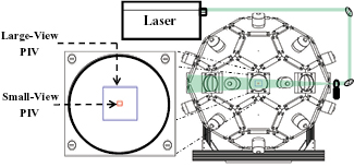
Figure 4. Two-scale PIV experimental setup. The laser beam travels through optics to form a light sheet that illuminates the center plane in the flow chamber. The window is enlarged in the figure to show the scaled sizing of the two PIV views (small-view: 7.1 mm × 5.7 mm, large-view: 48.6 mm × 43.3 mm).
Download figure:
Standard image High-resolution imageThe two PIV systems share the same laser and optical setup in order to ensure that images are obtained from the same plane. The laser was a Solo-PIV miniLase III, providing a light sheet at a thickness around 1 mm through a spherical and a cylindrical lens. The two PIV image acquisition systems had different hardware, as described below. The small-view PIV system consisted of an IDT SharpVision 1300-DE camera (1280 × 1024 pixel resolution, 8-bit, double exposures at 10 Hz) attached to an Infinity-USA K Series long-distance microscope for image capturing. The small-view PIV camera and the laser were synchronized by the IDT Provision PIV software and an IDT timing hub. The large-view PIV system used a PCO 4000 CCD camera (3000 × 2672 pixel resolution, 14 bit, double exposures at 2 Hz) with a Nikon-NIKKOR 200 mm f/4 D Close-Up Lens. The large-view PIV camera and the laser were synchronized by two Stanford Pulse Generators, and PCO CamWare software was used to capture images. The PIV cameras determine the data acquisition frequencies for each setup: 10 image pairs per second for the small-view PIV and 2 image pairs per second for the large-view PIV. The laser double-pulse frequency was adjusted accordingly for the two setups. The distance between the camera lens and the visualization window was fixed at 10 cm. Under this condition, the small-view and large-view PIV systems had magnification factors (physical dimension divided by the image dimension) of 0.83 and 1.8, respectively.
We used aluminum powder particles of  diameter (
 as tracer particles. These particles were injected into the chamber by a solid particle nozzle mounted on top of the apparatus while the fans were running at given rotating speeds. We chose PIV exposure time delay (
 ) based on the criteria given in equation (8.88) by Adrian and Westerweel [26]. PIV images from both systems were processed using an in-house modified version of the open-source MatPIV 1.6.1 code [30], with 50% overlap of interrogation cells. Interrogation cell size was determined by changing the size of interrogation cell from 28 × 28 pixels to 98 × 98 pixels with 10 pixels increments. It was found that at 48 × 48 pixels, the small-view PIV image pairs produced the clearest distinguishable peaks during image-pair cross-correlation, and the averaged signal-to-noise ratio (SNR)—the height of the primary peak and the height of the second tallest peak—was 2.47. The large-view PIV image pairs produced the clearest, distinguishable correlation peaks when interrogation cell size was 28 × 28 pixels, which gave an averaged SNR of 3.91. We subsequently processed PIV images using these pixel sizes. These corresponded to resolved cell sizes of
 and
and  in the chamber for the small- and large-view PIV setups, respectively. Furthermore, we determined measurement uncertainties of the two-scale PIV system based on the SNR of PIV image pairs [31]. For the small- and large-view PIV measurements, the uncertainties were
  0.12 pixel and
  0.10 pixels, corresponding to
  4% and
  5% of turbulence RMS velocity fluctuation uncertainty, respectively.
Although our 'soccer ball' chamber is equipped with two visualization windows on opposite sides of the chamber, due to confinement of laboratory space, the small-view and large-view PIV measurements were taken through only one window sequentially under identical flow conditions to provide turbulence statistics.
3.3. Repeatability confirmation
Before performing turbulence characterization, we checked the statistical repeatability of flow in the HIT chamber. If the turbulence in the apparatus is statistically repeatable under a given operating condition, then temporal averaging can be carried out instead of ensemble averaging to reduce the cost of experiments. To that end, we took 6 independent time series of PIV measurement using the small-view PIV system at the fan speed of 3000 RPM. In each time series, we collected 500 PIV image pairs continuously and analyzed velocity statistics (mean velocity and turbulence strength) at the center of the field of view. These statistics were compared across the 6 individual tests to check for measurement consistency.
3.4. Data acquisition for turbulence characterization
During HIT turbulence characterization, we performed PIV measurements under 6 flow conditions inside the chamber: varying fan speed from 1500 RPM to 3500 RPM in an increment of 500 RPM provided 5 flow conditions, and an additional fan speed of 3250 RPM was also included to increase the data density in the higher end of  . To avoid perturbation of the flow from particle injection, PIV data were only recorded after the particle injector had been closed for at least 60 s.
Under each flow and PIV recording condition, PIV measurements were taken in 10 separate runs with an ample time lapse in between, instead of continuously. This approach helped minimize the temperature rise in the flow chamber from heating due to fan operation. The length of the time window for each data collection run was determined by the CCD camera memory. The small-view PIV camera allowed for a batch of 500 image pairs to be recorded and transferred to the computer each time. Its framing rate was 10 image pairs per second. Therefore, each run lasted 50 s. For the large-view PIV measurements, the camera allowed for a batch of 200 image pairs to be recorded and transferred. Its framing rate was at 2 image pairs per second. Therefore, each run lasted 100 s. We have determined that within a 100 s run, the air temperature inside the chamber did not increase significantly. Under the highest fan speed (3500 RPM), the maximum temperature rise was  , corresponding to
  increase in air viscosity. Between runs we allowed sufficient time for the facility to cool down to room temperature. In order to determine if the convergence of turbulence statistics was achieved within one run, we plot the mean velocity and turbulence strength against the image pair recording time, both for small-view and large-view PIV.
3.5. Homogeneous and isotropic region
The size of homogeneous and isotropic region and the degree of homogeneity and isotropy are two important considerations of our HIT chamber (see section 2.3). The whole-field flow measurement capability of PIV allowed us to examine the spatial distributions of homogeneity index  and isotropy index
  . We employed the large-view PIV measurement (field of view
  ) to quantify the homogeneous and isotropic size and degree of homogeneity and isotropy of our new flow facility. To describe the spatial domain in the flow field, we introduced a Cartesian coordinate system with the origin point at the geometrical center of the chamber, which was also the center of the PIV view. The X- and Y-axes were along the horizontal and vertical directions, respectively.
By applying equations (1) and (2) at each PIV interrogation cell, we were able to measure homogeneity index  and isotropy index
  distribution in the field of view. At each interrogation cell, we calculated
  and
and  ensemble-averaged over 10 large-view PIV runs. The data presented in section 4.3 was collected at fan speed of 3000 RPM. We found that up to 3500 RPM of fan speed, the test data of
  and
and  displayed no significant differences with respect to fan speed.
3.6. Turbulence dissipation rate estimation
A challenge in characterizing turbulence in a flow facility is the estimation of turbulent kinetic energy dissipation rate  . Options for estimating
  include the scaling argument method [32], spectral fitting method [3, 33, 34], direct method [35–37], large eddy PIV method [38], and the structure function fit method [39]. We discussed in detail the performance of these different methods for estimating
  from PIV velocity field measurements in our previous HIT chamber [12]. We concluded that the
  -corrected, second-order longitudinal velocity structure function method was the most appropriate method to estimate the dissipation rate in homogeneous and isotropic turbulent flow [12]. Therefore, we adopted the same method in characterizing turbulence dissipation rate in our 'soccer ball' apparatus.
The longitudinal velocity structure function is defined as [12]

where  is the order of the structure function,
  is the separation vector of two fluid elements,
  is the unit vector which points in the direction of
  , and
, and  is the fluctuating velocity in the
  direction. When
  , equation (15) becomes the second-order longitudinal velocity structure function
  .
.
From Kolmogorov's first and second similarity hypotheses, in the inertial subrange the second-order structure function can be expressed as [2]

Note that this is valid only in the inertial subrange, i.e. when the separation distance  . Rearranging equation (16), we can express turbulence dissipation rate as
Where  is any separation distance in the inertial subrange, where
  is a constant. In order to determine
  , we can plot
 ![${{\left[\frac{{{D}_{LL}}(r)}{{{C}_{2}}\left({{R}_{\lambda}}\right)}\right]}^{\frac{3}{2}}}\left(\frac{1}{r}\right)$](https://content.cld.iop.org/journals/0957-0233/27/3/035305/revision1/mstaa1221ieqn192.gif) as a function of
as a function of  . When it plateaus (reaches a constant), the constant value is taken as
  . Equation (17) provides foundation for estimating turbulence dissipation rate
  though the second-order structure function
  .
.
From  , we can calculate
  through Taylor microscale
  , which is related to dissipation rate
  as [1, 2]:

Plugging equation (18) into equation (3), we obtain

To calculate  and
and  using equations (17) and (19) respectively, we need to estimate the constant
  , which is dependent on the unknown
  . This implicit equation set can be solved by iteration. We assumed an initial value
  [40], which enabled the initial estimates of
  and
and  . Subsequent corrections to the constant
  were made by using figure 6 from Yeung and Zhou [41]. With the new, iterated values of
  , new estimates for
  and
and  were obtained. Final values of
  and
and  were obtained when the iteration results are within 1% differences between successive iterations.
It should be noted that calculating dissipation rate  and
and  through velocity structure function requires instantaneous velocity measurement at two points separated by a distance
  . Furthermore, the separation distance
  also needs to be varied to give
  , and subsequently
  in the inertial subrange. The use of PIV is intrinsically more advantageous than LDV for getting instantaneous multi-point velocity measurements for this purpose.
4. Experimental results
In what follows, we present results of turbulence characterization and confirmation of homogeneity and isotropy from the two-scale PIV measurements. We performed crosschecks of experimental results from the two independent PIV measurements from the small- and large-view PIV systems to ensure accuracy and reliability.
4.1. Statistical repeatability
Figure 5(a) shows the time-averaged velocity components  at the center of field of view from six independent tests. These mean velocity values were all within 0.1 m/s from zero, which is negligible compared to the turbulence strength of 1.33
  . This reflects the 'nearly zero-mean' characteristics of the HIT chamber. There was no preferred sign for the residual mean velocity. Furthermore, turbulence strength values from different tests, plotted in figure 5(b), were within 5% from each other. We thus conclude that our apparatus has acceptable statistical repeatability.
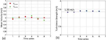
Figure 5. Turbulence mean velocity and turbulence strength in six time series, measured by the small-view PIV ( ). (a) Mean velocity. (b) Turbulence strength.
Download figure:
Standard image High-resolution image4.2. Statistical convergence
Figure 6 plots the mean velocity and turbulence strength at the center of field of view as a function of PIV recording time through one single run, both for small- and large-view PIV measurement. It is evidenced that the convergence of turbulence statistics is achieved by the end of the experimental run (500 and 200 image pairs for the small- and large-view PIV setups, respectively). Moreover, all the turbulence statistical characterizations described later in this paper are calculated based on larger sample sizes, 2000 and 5000 image pairs for small- and large-view PIV, respectively.

Figure 6. Turbulence mean velocity and strength against time from the small- and large-view PIV measurement at  . Data were recorded at 10 and 2 image pairs per second, respectively, to a total of 200 and 500 image pairs in each run. (a) Mean velocity components based on small-view PIV. (b) Mean velocity components based on large-view PIV. (c) Turbulence strength based on small-view PIV. (d) Turbulence strength based on large-view PIV.
Download figure:
Standard image High-resolution image4.3. Mean velocity and turbulence strength
After the statistical repeatability test, we carried out the entire turbulence characterization as described in sections 3.4–3.6. Figure 7 plots the mean flow velocity  and
and  in the horizontal and vertical directions, respectively, from both PIV measurements, for all six fan speeds. The mean velocity was essentially zero at low fan speeds. Deviations from zero increased with increasing fan speeds to a maximum of
  .
.
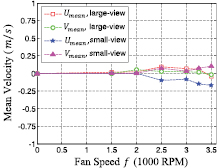
Figure 7. Turbulence mean velocity (two components) versus fan speed  from the two-scale PIV measurement.
Download figure:
Standard image High-resolution imageFigure 8 plots turbulence strength  from both small- and large-view PIV measurements against fan speed
  , demonstrating a linear dependence. Separate linear regressions were performed for the small- and large-view data, producing almost identical linear fits. The highest
  was 1.57 m s−1 under the highest fan speed of 3500 RPM. The linear dependence of the measured
  on fan speed provides strong experimental support for equation (8) (i.e. linear relationship of turbulence kinetic energy to individual fan velocity), which was a key assumption for our derivation of the
  expressions in equations (10) and (12). Recall the argument for equation (8) was: The turbulent kinetic energy
  in the center of the HIT chamber should be proportional to the kinetic energy input from all the actuators,
  , due to energy conservation. Note that
  and
and  , as shown in equation (11). Thus the energy argument
  is equivalent to
  . This linear relation of turbulence strength on fan rotational speed is confirmed by the experimental results shown in figure 8.
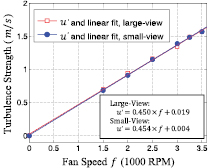
Figure 8. Turbulence strength versus fan speed  found from the two –scale PIV measurement.
Download figure:
Standard image High-resolution image4.4. Homogeneous and isotropic region
Figure 9 shows a spatial distribution of the homogeneity index  ensemble averaged from 10 runs of large-view PIV, with figure 9(a) showing 2D distribution of
  and figure 9(b) showing
  value plotted along the horizontal line
  . We can see that
  with a small range of fluctuations (0.97–1.02), indicating that the HIT chamber provides a high degree of homogeneity. Using the criterion of
  , we can see that 'homogeneous region' existed in a region of at least
  about the center of the chamber.

Figure 9. Homogeneity index  obtained from the large-view PIV measurement at fan speed of 3000 RPM. (a) Distribution in a 2D plane; (b) Distribution along horizontal line
  . The shaded area indicates the homogeneity region based on
  . It covered the entire field of view of the large-view PIV, with a linear dimension of
  .
.
Download figure:
Standard image High-resolution imageFigure 10 shows the measurement results of isotropy index  distribution, ensemble-averaged over 10 large-view PIV runs, where figure 10(a) shows 2D distribution of
  and figure 10(b) shows
  along the horizontal line
  . We can see
  with a small range of fluctuations (0.95–1.03), which indicates that the HIT chamber provides a high degree of isotropy. Using the criterion of
  , we can see that 'isotropic region' existed in a region of
  in the center of the chamber.
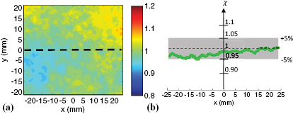
Figure 10. Isotropy index  obtained from large-view PIV measurement at fan speed of 3000 RPM. (a) Distribution in a 2D plane; (b) Distribution along horizontal line
  . The shaded area indicates the isotropy region based on
  . It covered the entire field of view of the large-view PIV, with a linear dimension of
  .
.
Download figure:
Standard image High-resolution imageAssuming spherical symmetry of the apparatus, we infer that the homogeneous and isotropic region is a sphere with a diameter of  at the center of the chamber. This is a significant improvement over our previous cubic chamber (
 ), both size and quality [42].
4.5. Turbulence dissipation rate
In order to estimate turbulence dissipation rate  using equation (17), we calculated the second-order longitudinal velocity structure function
  using equation (15), where
  was varied along the
  direction. This was done for all experimental conditions. In order to determine the inertial subrange and thus
  , we plotted the compensated longitudinal second-order structure function
 ![${{\left[{{D}_{LL}}(r)/{{C}_{2}}\left({{R}_{\lambda}}\right)\right]}^{\frac{3}{2}}}\left(\frac{1}{r}\right)$](https://content.cld.iop.org/journals/0957-0233/27/3/035305/revision1/mstaa1221ieqn269.gif) against separation distance
against separation distance  . When it plateaus (reaches a constant), the constant value is taken as
  according to equation (17). Any
  in the range of the plateau (inertial subrange) gives the same result of
  . Figures 11(a) and (b) show these functions under different fan speeds for the small-view and large-view PIV measurements, respectively. All
  values are marked on the axes on the right of the plots.

Figure 11. Compensated second-order longitudinal velocity structure functions ![$(1/r){{\left[{{D}_{LL}}(r)/{{C}_{2}}\left({{R}_{\lambda}}\right)\right]}^{\frac{3}{2}}}$](https://content.cld.iop.org/journals/0957-0233/27/3/035305/revision1/mstaa1221ieqn275.gif) (the left vertical axis) for all flow conditions for determining turbulence dissipation rate
(the left vertical axis) for all flow conditions for determining turbulence dissipation rate  (on the right axis in m2/s3). (a) From the small-view PIV. (b) From the large-view PIV.
Download figure:
Standard image High-resolution imageComparing figures 11(a) and (b), we see that the small-view and large-view PIV measurements yielded similar dissipation rate values. However, the large-view measurement accounted for a much larger separation distance r. To compare the measured dissipation rate as a function of fan speed for both sets of PIV measurement, we generated figure 12, which demonstrates an excellent agreement across all flow conditions from the two PIV views. Power fit was used to find the relation between dissipation rate  and fan speed
  . Exponents of the curve-fitting results were found to be 2.83 (small-view PIV) and 2.54 (large-view PIV). This experimental result is roughly consistent with the scaling argument of dissipation rate in equation (4), where
  is proportional to the turbulent kinetic energy
  to the power 3/2, and thus to
  , as well as to
  , to the power 3. This consistency suggests that our two independently measured dissipation rates from the two-scale PIV system are reasonable and in agreement with each other.

Figure 12. Measured turbulence dissipation rate  versus fan speed
  .
.
Download figure:
Standard image High-resolution image4.6. Taylor-microscale Reynolds number dependence on fan speed
Based on the relationship between  and
and  given in equation (19), we calculated
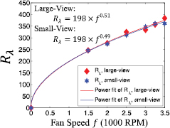
  for each flow condition using both PIV views. The results are plotted as
  versus fan speed in figure 13. Power fit was used to find the experimental relationship between
  and fan speed, showing exponents to be 0.49 (small-view PIV) and 0.51 (large-view PIV). A good agreement between the two PIV measurements was achieved. These experimental results also lend strong support to equation (12), the
  equation we derived theoretically and used for our chamber design. Equation (12) predicted that
  scales with the rotational fan speed
  to the power of 0.5.
Figure 13. Measured  versus fan speed
  .
.
Download figure:
Standard image High-resolution image
The experimentally validated square-root dependence of  actually reflects a well-known scaling that
  is proportional to the square root of the integral-scale Reynolds number
  , as shown in equation (6) as well as in Pope [2]. In wind tunnels,
  is proportional to the inlet flow speed and thus to the fan (blower) speed of the wind tunnel. Here, we have shown both theoretically and experimentally that a fan-driven enclosed chamber also follows a square-root relationship between
  and fan speed.
Since the large-view PIV measurement accounted for a larger portion of the homogeneous and isotropic field compared to small-view PIV measurement, and since it agreed rather well with the latter, we used the large-view PIV results as the basis for calculating other turbulence quantities.
The  in the 'soccer ball' chamber at the maximal fan speed was calculated to be
  , which is within 7.5% difference from the theoretical prediction of
  This agreement again supports equation (12)—our theoretical relationship between
  and physical parameters of a fan-driven HIT chamber. The
  levels measured in our apparatus match the current DNS capabilities.
4.7. Full turbulence characterization
Table 1 shows the full turbulence characterization of the 'soccer ball' chamber under all six different flow conditions from large-view PIV measurement. From the mean velocity values, we can see that near-zero-mean flow is achieved across all fan speeds in our chamber. From the Froude number values, we can see that the fan-generated turbulence acceleration at the Kolmogorov scale was 4.4–25.0 times of the acceleration of gravity, which indicates that the gravity effect on inertial particles was insignificant compared to the turbulence effect in our chamber. It is also seen that, as fan speed increased, turbulent kinetic energy dissipation rate increased, while the Taylor microscale and Kolmogorov length/time scales decreased.
Table 1. Full turbulence characterization in the 'soccer ball' HIT chamber.
| Fan speed (RPM) | 1500 | 2000 | 2500 | 3000 | 3250 | 3500 |
|---|---|---|---|---|---|---|
 |
0.68 | 0.93 | 1.16 | 1.35 | 1.47 | 1.56 |
 |
0.72 | 0.95 | 1.17 | 1.32 | 1.51 | 1.56 |
 |
0.02 | 0.02 | 0.09 | 0.07 | 0.06 | -0.04 |
 |
0.01 | 0.06 | 0.03 | 0.02 | 0.02 | -0.02 |
Turbulence strength,  |
0.70 | 0.94 | 1.16 | 1.33 | 1.49 | 1.56 |
Turbulent kinetic energy, ( ( |
0.73 | 1.33 | 2.03 | 2.67 | 3.32 | 3.65 |
Eddy turnover time,  |
7.9 | 4.9 | 3.8 | 2.9 | 2.5 | 2.5 |
Dissipation rate,  |
3.6 | 9.2 | 16.5 | 27.0 | 35.9 | 47.0 |
Large eddy length scale,  |
0.18 | 0.16 | 0.18 | 0.17 | 0.17 | 0.18 |
Large Eddy Time Scale,  |
0.24 | 0.18 | 0.15 | 0.13 | 0.11 | 0.11 |
Kolmogorov length scale,  |
179 | 141 | 123 | 109 | 101 | 100 |
Kolmogorov time scale,  |
2.0 | 1.3 | 1.0 | 0.8 | 0.7 | 0.6 |
Kolmogorov velocity scale,  |
0.09 | 0.11 | 0.13 | 0.14 | 0.16 | 0.16 |
Taylor Microscale,  |
5.5 | 4.6 | 4.4 | 3.9 | 3.8 | 3.9 |
Froude number,  |
4.4 | 8.9 | 13.4 | 19.3 | 24.2 | 25.0 |
Taylor-microscale Reynolds number,  |
246 | 277 | 324 | 334 | 357 | 384 |
The Kolmogorov length scale  varied from 179 to 100
  in the HIT chamber. The PIV measurement interrogation cell sizes (
 for large and
  for small-view) were both smaller than 5
 , thus satisfying the spatial resolution requirement for PIV measurement in turbulence [27].
5. Discussions—comparison with other enclosed HIT chambers
Upon comprehensive experimental characterization of our 'soccer ball' turbulence chamber, we performed a detailed comparison of our chamber and its turbulence characteristics against other published enclosed HIT chambers (table 2). Out of the seven chambers being compared, the current chamber features the second highest  the highest turbulence strength, the highest dissipation rate and Froude number, and thereby the smallest gravity effect. Moreover, our facility is the only one equipped with multiple orientations for flow visualization and PIV measurement.
Table 2. Comparison of our HIT chamber with 5 enclosed chambers reported in the literature. Performance data are for the highest flow conditions.
| Hwang and Eaton [3] | Lu et al [8] | de Jong et al [12] | Goepfert et al [9] | Chang et al [10] | Bewley et al [43] | Present Chamber | |
|---|---|---|---|---|---|---|---|
| Geometry | Cube | Cube | Cube | Cube | Truncated Icosahedron | Truncated Icosahedron | Truncated Icosahedron |
| Wall material | Plexiglas | Plexiglas | Acrylic | Open wall | Wood | Acrylic | Aluminum |
| Actuator number | 8 | 8 | 8 | 8 | 32 | 32 | 20 |
| Actuator type | Synthetic jet | Synthetic jet | Fans | Synthetic jet | Synthetic jet | Synthetic jet | Fans |
| Actuator orifice diameter (cm) | 4 | — | 11 | 20 | 4.3 | 6 | 16 |
| External size (cm) | 41 | 50 | 40 | 90 | 99 | 100 | 100 |
| Homogeneous and isotropic region size (cm) | 3.2 | N/A | 2.2 | 5.0 | 5.0 | 5.0 | ⩾4.8 |
 (m/s) (m/s) |
0.87 | 0.6 | 1.07 | 0.88 | 1.1 | - | 1.57 |
Dissipation rate  ( ( |
11.0 | 1.4 | 38.7 | 5.8 | 6.7 | 3.2 | 38.3 |
Kolmogorov length scale   |
130 | 220 | 97 | 155 | 155 | 180 | 100 |
Froude number  |
9.8 | 2.1 | 25.1 | 6.1 | 6.8 | 3.8 | 25.0 |
| Gravity effect |
10.2% | 47.6% | 4.0% | 16.4% | 14.7% | 26.7% | 4% |
 |
220 | 260 | 184 | 250 | 481 | 190 | 384 |
aGravity effect here is measured by the acceleration of gravity normalized by the Kolmogorov-scale acceleration, or the inverse of Froude number.
From table 2, it can be noted that larger chambers are generally associated with more actuators, a larger homogeneous and isotropic region and higher  . Fan-driven chambers produce far higher turbulence dissipation rates than loudspeaker-driven chambers, thus leading to significantly less gravity effect.
6. Limitations of this study
This study presents a new enclosed turbulence chamber and its flow characterization by PIV measurement. The chamber design has several limitations and so does our measurement.
First, the original goal for our study was to achieve  in our HIT chamber to match with capabilities of leading DNS. By the time we completed the construction and testing of this apparatus, DNS ability had advanced further. However, the achieved
  is still on the high end of both experimental and DNS capabilities. Furthermore, recent DNS studies of particle-laden turbulence found that
  is a weak factor on particle collision compared to gravity [44, 45]. We therefore aimed at minimizing the effect of gravity while achieving a sufficiently high
  in our HIT chamber. This goal has been achieved in this study.
Second, although the use of fans alleviates the problem of gravitational settling of particles, which is greatly advantageous for studies of particle-laden flow in homogeneous and isotropic conditions as well as for PIV measurement (which uses tracer particles), it also compromises the achievable Taylor micro-scale Reynold number,  . As mentioned above, fan-driven turbulence in a near-zero-mean enclosed chamber generates higher dissipation rate compared to its loudspeaker-driven counterpart. However, this drawback can be remedied by increasing the number of fans, increasing the size of the chamber, or increasing the jet velocity (thus power of the motors).
Third, in our testing of the HIT apparatus we have noticed that when the fans were operated within 3325–3425 RPM, the chamber vibrated drastically due to resonance. The vibration sharply increased when the fan frequency past 3325 RPM and returned to normal immediately past 3425 RPM. Operation under the resonance condition over prolonged periods of time could damage the facility and thus should be avoided. Therefore, when designing an enclosed flow facility in the future, the resonance frequency of the apparatus should be estimated and shifted away from the intended operating condition by adjusting the structure and material.
Fourth, the interior of our HIT chamber is difficult to access. We recommend for future designs to construct the chamber in two fastened halves that can be easily separated, or to connect the facets with hinges instead of screws to allow quick and convenient disassembling.
Fifth, equation (12) suggests that  scale with the number of fans (
 ) to the 1/4 power. We were unable to experimentally verify this important scaling relation in this paper, as it is impossible to shut off a fraction of the fans in our chamber while keeping the rest symmetrically distributed.
Finally, our two PTV setups were not performed simultaneously, due to laboratory space limitation. Therefore it was not possible for us to obtain and crosscheck instantaneous velocity field measurements from the two image acquisition systems in real time.
7. Suggested potential applications of enclosed HIT flow chambers like this one
This work was motivated by a need to conduct experimental studies of particle dynamics in homogenous and isotropic turbulent flow, with particular focus on inertial particle clustering [6] and inter-particle relative velocity [15, 46]. However, such an enclosed HIT flow facility can also be used for studying additional fundamental particle-laden flow problems with important applications, e.g. particle collision in homogeneous and isotropic flows [47], particle dynamics in decaying turbulence [3] and particle dynamics in anisotropic turbulent flows [10].
Further applications involve slight modifications of the apparatus. For example, the system can be equipped with a corona discharge unit [48–50] to electrically charge particles and study behavior of charged particles subjected to both an electric field and turbulent flow. Such fundamental study will shed light on the competing influence of the Coulomb force and drag force on particle clustering and collision in rain producing clouds [51, 52]. This knowledge has important implications in rain enhancement [48, 53, 54]. This modified setup can also be used to study charged particle deposition, which may potentially help mitigating haze in cities [55, 56] and explain how aerosols spread in human lungs [18, 57, 58]. Moreover, given the redundancy of the axes of symmetry in our 'soccer ball' chamber, several of the fans can be replaced by combustion or mixing devices such as flame injectors, so as to observe turbulence effects on combustion, thermal diffusion, and stream mixing.
8. Conclusion
We have created a new, enclosed, highly symmetrical, fan-driven, truncated icosahedron HIT chamber with high  , high Froude number, and PIV interrogation capability. An explicit relationship between the Taylor microscale Reynolds number
  of the turbulent flow and the physical setup has been developed. We have characterized the base turbulent flow using a new two-scale PIV approach. High homogeneity and isotropy was achieved in a large central region (48 mm diameter) of the chamber. Using the second-order velocity structure function, we obtained turbulence dissipation rates and maximum
  , nearly achieving the design goal of
  . Experimental data confirmed that the turbulence strength increases linearly with fan speed, and
  is proportional to the square root of fan speed. The two-scale PIV approach effectively navigates the conflicting requirements of high spatial resolution and a large measurement area and provides cross-validation to improve measurement quality and ensure turbulence dissipation rate accuracy and
  . Creating and measuring high-Reynolds-number HIT flow in this near-zero-mean enclosed apparatus paves the way for future studies that are aimed at advancing our understanding and modeling of particle dynamics both experimentally and numerically.
Acknowledgments
This work was supported by the National Science Foundation through a Collaborative Research Grant CBET-0967407. We thank our collaborators Lance Collins and Peter Ireland of Cornell University for stimulating discussions, Xiaoqin Jiang for critical assistance in chamber design, Steve Capp for chamber assembly, and Adam Hammond for editorial assistance.