
Abstract
In situ stiffness adjustment in microelectromechanical systems is used in a variety of applications such as radio-frequency mechanical filters, energy harvesters, atomic force microscopy, vibration detection sensors. In this review we provide designers with an overview of existing stiffness adjustment methods, their working principle, and possible adjustment range. The concepts are categorized according to their physical working principle. It is concluded that the electrostatic adjustment principle is the most applied method, and narrow to wide ranges in stiffness can be achieved. But in order to obtain a wide range in stiffness change, large, complex devices were designed. Mechanical stiffness adjustment is found to be a space-effective way of obtaining wide changes in stiffness, but these methods are often discrete and require large tuning voltages. Stiffness adjustment through stressing effects or change in Young's modulus was used only for narrow ranges. The change in second moment of inertia was used for stiffness adjustment in the intermediate range.
Export citation and abstract BibTeX RIS

Original content from this work may be used under the terms of the Creative Commons Attribution 3.0 licence. Any further distribution of this work must maintain attribution to the author(s) and the title of the work, journal citation and DOI.
1. Introduction
Micro-electromechanical systems (MEMS) are microchips that integrate mechanical and electrical functionality onto a single device. Many of these MEMS have deformable structures where the stiffness is a key factor in the performance of the device. An example is the stiffness of the cantilever of an atomic force microscope (AFM) probe, where the stiffness should match the mode of operation and the mechanical properties of the sample. Design for stiffness is also very important for devices where the resonance frequency is the determining factor in the performance, because this is dependent on the stiffness ( , where
  ,
,  are effective stiffness and effective mass respectively). Eminent examples are radio-frequency (RF) filters, mass sensors, gyroscopes, energy harvesters.
The ability to adjust the stiffness after fabrication can provide great benefits to the performance of MEMS: it can compensate for manufacturing inaccuracies, influences of the operational environment (like temperature, humidity etc) or it can increase the operational range.
Several methods to achieve this change in stiffness are described in literature. However, an organized review of all these techniques is not available, which is addressed in this paper. Earlier, a review has been made on variable stiffness devices [1], however it does not cover MEMS. Furthermore, there are several reviews that cover frequency tuning in MEMS [2, 3], which is closely related to stiffness tuning (one of the approaches to tuning the resonance frequency is by tuning the stiffness). The present review only covers stiffness adjustment methods in MEMS and compares these devices on their stiffness adjustment capabilities. The stiffness change should be reversible, controllable and in situ (while the device is in operation). Some devices show stiffness tuning effects only in dynamic behavior [4, 5]. These devices are not addressed in this review. Stiffness adjustment covers both continuous tuning and discrete switching of stiffness; both are addressed in this review. The contribution of this paper is an overview on the state of the art of in situ stiffness adjustment in MEMS, organized by physical working principle, plus an analysis of advantages and disadvantages of existing methods. A categorization is defined, which is used throughout the paper to sort the literature. The results are summarized in a table and graph. These are intended to be a selection tool for designers that need stiffness adjustment capabilities in MEMS.
In the following sections, the methods used are explained, covering the search method, definition of the classification and key properties of the literature found. Next, the results are presented; they are summarized in a table and graph. Lastly, the results are discussed and the conclusions presented.
2. Methods
In this part the methods used for this review are presented. First the search method is discussed, followed by the categorization used and the key properties that are addressed.
2.1. Search method
Many devices that have stiffness adjustment capabilities are applied in resonance tuning applications. To get a complete overview, the search was not aimed only at stiffness tuning, but also at frequency tuning. Only the devices that achieved frequency tuning through stiffness tuning are included in the results, however. As an initial search the key words stiffness, compliance, spring constant, frequency were combined with tuning, adjusting, switching, changing, change, varying, softening, hardening. The references were also checked.
2.2. Categorization
The categorization was established to sort the literature found. This was done according to the physical working principle. Some of these categories also have sub-categories to differentiate distinctive methods that were used. The categorization can be found in table 1. The first group uses electrostatic effects to add a stiffness to the system. There are four different tuning methods that can be distinguished: Parallel plate, Varying gap, Varying electrode shape, Non-interdigitated comb fingers. These are further explained in section 3.1. The second group uses mechanical tuning, that can either be achieved by changing the effective length of the suspension or by engaging extra mechanical springs. These are addressed in section 3.2. The third category uses a change in the second moment of inertia to change the stiffness (section 3.3). The fourth group uses compressive, axial stressing effects for stiffness adjustments, that can be induced by piezoelectric elements, thermal expansion or electrostatic forces. This is discussed in section 3.4. The Young's modulus (elasticity of a material) has temperature dependency. So the stiffness, which is dependent on the Young's modulus, can be tuned by changing the temperature. This effect is used by the devices in the final category (section 3.5).
Table 1. Categorization of stiffness adjustment methods used in this review.
| Physical principle | Sub-category |
|---|---|
| Electrostatic | Parallel plate |
| Varying gap | |
| Varying electrode shape | |
| Non-interdigitated | |
| Mechanical | Change effective length |
| Engaging mechanical springs | |
| Second moment of inertia | — |
| Stressing effects | Piezoelectrically induced |
| Thermally induced | |
| Electrostatically induced | |
| Young's modulus | — |
2.3. Key properties
The performance of the devices is addressed according to several key properties. These key properties are used in table 2 to describe the devices. They are defined as:
- Unadjusted stiffness (k0): The stiffness of the system in the direction of motion, when no tuning voltage is applied (all of the mechanisms are voltage controlled).
- Change in stiffness (
 ): The difference between the unadjusted stiffness k0 and the tuned stiffness ktun. This can either be a positive or negative number, depending on whether the method increases or decreases the stiffness.
 - Normalized change in stiffness : The ratio between the highest and lowest achievable stiffness in the device. When the stiffness has decreased: , ; when the stiffness is increased , . A similar parameter was used in an earlier review [1].
- Tuning voltage (V): The voltage that is applied to the system in order to achieve the maximum stiffness adjustment effect.
- Size: The size of the system. In some of the literature found the size of the device is explicitly mentioned. When this is not the case, micrographs or schematics are used to make an estimate, if a reference scale is present.
- Relative Size: The relative size of the tuning mechanism with respect to the entire system, expressed as a percentage in steps of 20% (0–20, 21–40, 41–60, 61–80, 81–100). This is estimated from micrographs or schematics of the devices. The size of the tuning mechanism is defined as the amount of space it adds to the system; it is the difference between the size of the current system and the size it would have without stiffness tuning capabilities.
- Motion: MEMS are usually made out of silicon wafers. The motion of the device can either be in the plane of the wafer, or out of plane.


Table 2. Summary of in situ adjustable stiffness devices. Only devices for which the stiffness data was presented in or could be derived from the original literature are included in this overview.
| Physical principle | Subgroup and section | Reference | Untuned stiffness (N m−1) | Change in stiffness (N m−1) | Normalized change in stiffness | Tuning voltage (V) | Size | Relative size (%) | Motion |
|---|---|---|---|---|---|---|---|---|---|
| Electrostatic • | Parallel plate (section 3.1.1) | [6](a) | 17.41 | −16.79 | 28.08 | 46.1 | 0.065 mm2 | 81–100 | In plane |
| [7] | 29 | −9.4 | 1.48 | 50 |  mm mm |
21–40 | In plane | ||
| [8] | 24.4 | −13.4 | 2.22 | 53 | 250 μm(diameter) |
21–40 | Out of plane | ||
| [6](b) | 5.1 | −3.2 | 2.7 | 22.4 | — | 81–100 | In plane | ||
| [9] | 1.03 | −1 | 29 | 10 |  μm μm |
41–60 | In plane | ||
| [10] | 0.1338 | −0.03 | 1.32 | — |  μm μm |
0–20 | Out of plane | ||
| (nanoresonator) (3.1.1) | [11] | 0.09 | 0.027 | 1.3 | 0.58 |  104 nm 104 nm |
— | Out of plane | |
| Varying gap (3.1.2) | [12] | 0.6 | −0.05 | 1.11 | 29 |  μm μm |
0–20 | In plane | |
| [13] | 17.3 | −1 | 1.06 | 60 |  μm μm |
81–100 | In plane | ||
| [14](a) | 0.47 | −0.47 |  |
80 | — | 41–60 | In plane | ||
| [14](b) | 0.47 | 0.28 | 1.60 | 90 | — | 41–60 | In plane | ||
| [15] | 2.64 | −2.11 | 5 | 150 |  μm μm |
81–100 | In plane | ||
| Varying electrode surface (3.1.3) | [16] | 0.76 | −0.36 | 1.9 | 40 |  μm μm |
21–40 | In plane | |
| [17] | 17 | 3.7 | 1.21 | 30 |  μm μm |
41-60 | In plane | ||
| [18] | 0.30 | 0.02 | 1.07 | 20 | 1 mm2 | 61–80 | In plane | ||
| [19](a) | 6.1 | 1.45 | 1.24 | 120 | — | 41–60 | In plane | ||
| [19](b) | 4.3 | −1 | 1.30 | 90 | — | 41–60 | In plane | ||
| [20](a) | 2.09 | −1.89 | 8.04 | 35 | 8.78 mm2 | 81–100 | In plane | ||
| [20](b) | 17.59 | −2.9 | 1.20 | 35 | 8.78 mm2 | 81–100 | In plane | ||
| Non-interdigitated (3.1.4) | [21](c) | 2.6 | −2.69 |  |
56.6 |  μm μm |
61–80 | In plane | |
| [21](d) | 2.6 | 5.2 | 3 | 72.1 | — | 81–100 | In plane | ||
| Mechanical |
Effective length (3.2.1) | [22] | 3.2 | 17.7 |
6.6 | 240 |  μm μm |
61–80 | In plane |
| Mechanical springs (3.2.2) | [23] | 0.01 | 0.09 |
10 | 130 |  μm μm |
61–80 | In plane | |
| Stressing effects □ | Thermal (3.4.2) | [24](a) | 0.2 | 0.22 | 2.1 | 6 |  μm μm |
0–20 | In plane |
| [24](b) | 0.2 | −0.04 | 1.25 | 6 |  μm μm |
0–20 | In plane | ||
| [24](c) | 0.69 | 0.8 | 2.15 | — | — | 0–20 | In plane | ||
| Young's modulus ◊ | (3.5) | [25] | 84.1 | −1.84 | 1.02 | 7.7 |  μm μm |
0–20 | In plane |
*Estimated from provided data. aDeflecting beam only. bDiscrete system. cExperiments show zero stiffness after tuning. Note: The definition of the performance indicators can be found in section 2.3. The reference in the table corresponds to both the number in the bibliography and that used in figure 1. A letter between parentheses in the reference column indicates that more than one device is included from a single reference.
2.4. Deriving the change stiffness from change in resonance frequency
A lot of the concepts that are discussed in this section are designed to change the resonant frequency rather than to change the stiffness; it is not always possible to find the stiffness of the devices in these papers. In cases where both the unadjusted and adjusted resonant frequencies are known, and the (effective) mass remains constant, it is possible to determine the ratio between unadjusted and adjusted stiffness. The effective mass of the system is expressed as a function of the effective stiffness and resonance frequency, set equal for the high and low stiffness states of the system. When the untuned stiffness is known, the tuned stiffness can be derived.


Here f is the resonance frequency, keff the effective stiffness and meff the effective mass. The subscripts 'high', 'low' are used to indicate the high and low stiffness states of the system.
3. Results
The results are sorted according to the categorization that was defined in section 2.2. For each category the theory behind the working principle is explained in the introduction and examples found in literature given. The examples are briefly explained; for more details the original papers can be consulted. In table 2 the literature found and its performance indicators are summarized. In figure 1 the devices are presented, where the relation between the change in stiffness and normalized change in stiffness are indicated. The devices for which the unadjusted stiffness or change in stiffness could not be found or calculated are not included in this graph or table. The colors and symbols used in the table correspond to those used in the graph. This provides a tool to select a concept for a specific application.
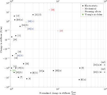
Figure 1. Change in stiffness versus normalized change in stiffness. The normalized stiffness is the largest achievable stiffness khigh divided by the lowest achievable stiffness  . The vertical axis is the change in stiffness, which can be positive or negative depending on whether the stiffness is higher or lower than the initial stiffness respectively. Devices that combine a large change in stiffness with a low normalized change in stiffness have a large untuned stiffness. Devices that combine a low change in stiffness with a large normalized change in stiffness have a low untuned stiffness. This figure provides insight in the stiffness tuning capabilities of the devices described. It provides a tool for designers of MEMS that require stiffness tuning to select a concept or suitable method that matches with the intended stiffness tuning range. Other important properties like size, relative size of the tuning mechanisms, tuning voltage and the direction of motion are shown in table 2. The numbers used in the graph correspond to those used in that table, and the references of this article. The colors and symbols represent devices that use the same physical principle. Devices [14](a) and [21](c) approach zero stiffness, so the normalized stiffness goes to infinity.
Download figure:
Standard image High-resolution image3.1. Electrostatic
Electrostatic stiffness adjustment relies on the fact that electrostatic forces are strong at micro scales, compared to other forces like gravity and inertial forces. In general, these concepts comprise a moving mass that is suspended by flexures. Electrodes are attached to the moving mass and are in close proximity to stationary electrodes. By applying a voltage between the stationary and moving electrodes, it is possible to exert a force on the mass. The electrodes will move, such that the electrostatic forces are in equilibrium with the mechanical restoring forces. In this new equilibrium, the stiffness has changed compared to its original state. There are four configurations for adding electrostatic stiffness to a system: parallel plate (section 3.1.1), varying gap method (section 3.1.2), varying surface method (section 3.1.3) and non-interdigitated comb fingers (section 3.1.4). Furthermore nano-resonators with electrostatic stiffness tuning are discussed under parallel plate mechanisms (section 3.1.1). The theory behind the four configurations is explained in the corresponding sections.
3.1.1. Electrostatic: parallel plate.
Two capacitive plates, separated by gap g0, a potential difference V and an overlapping surface  , are shown in figure 2. The bottom plate is fixed, and the top plate can move in both x and y directions. The capacitance between two electrodes is defined as:
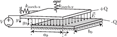
Figure 2. Two conductive plates, that have overlapping surface  , gap g0, with potential difference V. The charges (+Q and −Q) accumulate on the plates and form the electric field
  . The bottom plate is fixed; the top plate can move in x and y directions. Mechanical springs are attached to the top plate.
Download figure:
Standard image High-resolution imageThe amount of energy U, stored between capacitive plates can be calculated with:
The force on the top plate can be found by taking the derivative of the energy with respect to the direction of interest. The stiffness is found by taking the derivative of this force.
When a voltage is applied to the system, the parallel plates will move such that there is an equilibrium between the electrostatic attraction and mechanical restoring force. Around this new equilibrium position the stiffness is determined by sum of the mechanical and the electrostatic stiffness. The two capacitive plates have a (non-linear) stiffness in the y-direction, but have zero stiffness in x-direction. This electrostatic stiffness in the y-direction is used in parallel plate devices. Because the electrostatic stiffness is in the direction opposite that of the mechanical restoring force it is commonly called a 'negative'-stiffness. (For a positive displacement in y, the electrostatic force increases positively, while the mechanical restoring force increases negatively).
The amounts of electrostatic force and stiffness depend on the surface area, as shown in equations (6)–(9). So in order to have a significant effect without the need to further increase the voltage, the surface of the electrodes is often increased by applying a comb-like design as shown in figure 3.
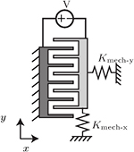
Figure 3. Two capacitive plates with combs to increase the surface area.
Download figure:
Standard image High-resolution imageParallel plate electrostatic tuning was reported by Adams et al [6]. The device is shown in figure 4. A tuning voltage is applied between the stationary and moving plates of the capacitor. With this design, a device with a resonance frequency of 21 kHz was reduced to 7.7% of its nominal value. The estimated mass of the system is  kg. So the mechanical stiffness of the system can be calculated by using equation (1). This gives a stiffness of 17.41 N m−1. The measured electrostatic stiffness coefficient
  is
is  N m−1 V−2, so for a tuning voltage of approximately 46 V (estimated from figure 5), this gives an electrostatic stiffness of:

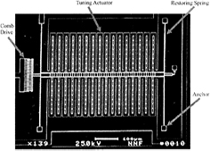
Figure 4. SEM image of mechanical oscillator with a symmetric, parallel-plate actuator. A comb drive and a displacement indicator are attached to the outer sides of the left and right restoring springs respectively. Reproduced with permission from [6]. © 1998 IOP Publishing.
Download figure:
Standard image High-resolution image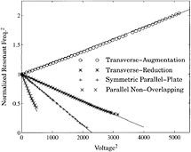
Figure 5. Experimental data for all four tuning actuators. The solid lines are least-squares fits to the first 10% of each data set. Normalizations are based on each oscillator's individual resonance frequency. Reproduced with permission from [6]. © 1998 IOP Publishing.
Download figure:
Standard image High-resolution imageMore devices were presented in this paper and are discussed later in this section, in sections 3.1.2 and 3.1.3. Each device is separately mentioned in table 2. The parallel plate design is marked with (a). The measurement results for these four devices can be found in figure 5.
A similar device was presented by Horsley et al [7]. A parallel plate comb drive adds an electrostatic stiffness of  N m−1 to the mechanical suspension of 29 N m−1. Parallel plate tuning was also applied by Torun et al [8], to tune the stiffness of a membrane that is used for force spectroscopy applications. The stiffness was reduced from 24.4 N m−1 to 11 N m−1.
The parallel plate tuning mechanism of figure 4 has a limited range of motion. When the gap between the stationary and moving electrodes becomes too small, the electrostatic attraction forces will become larger than the mechanical restoring force. The plates will collide and destroy the device. In order to increase the range of motion, Adams et al [6] applied parallel plate tuning with a branched finger design instead of having straight fingers, as shown in figure 6. When the position of the mass changes, the suspended combs move into the entrance region of the stationary combs. In order to achieve a linear behavior in positive and negative moving directions, a symmetric setup is used, such that the comb fingers will penetrate an entrance region in both directions of motion. The range of motion is increased from 0.8 μm to 1.3 μm compared to the previous design, while the efficiency remains approximately equal. The untuned resonance frequency is 7.5 kHz and the mass is  kg. So the mechanical stiffness of the system is 5.1 N m−1 according to equation (1). The experimental electrostatic stiffness is
  N m−1 V−2, resulting in a change in stiffness of
  N m−1 for 500 V−2 which is estimated from figure 5. A similar design was presented by Park et al [9]. The untuned and tuned resonance frequencies are 5.12 kHz and 0.950 kHz respectively. The theoretical proof mass weight is 1μg, so this yields an untuned stiffness of 1.03 N m−1 and a tuned stiffness of 0.04 N m−1 for a tuning voltage of 10 V.
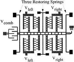
Figure 6. Schematic diagram of the parallel-reduction tunable oscillator. Reproduced with permission from [6]. © 1998 IOP Publishing.
Download figure:
Standard image High-resolution imageParallel plate tuning has been applied in a MEMS gyroscope by Sonmezglu et al [26]. The gyroscope has two vibrating modes (in x- and y-direction, in plane) and the resonance frequencies of these modes should be as close as possible. But due to manufacturing errors or temperature influences, there is usually a mismatch between these resonance frequencies. So by tuning the stiffness in one of these modes, the frequency can be tuned, such that it matches the other mode. A normalized change in stiffness of 1.30 is achieved, according to equation (3).
Parallel plate stiffness tuning is also applied without the commonly used comb structures. Yao et al [27] and Evoy et al [28] used flat electrodes under a suspended out-of-plane resonator to apply electrostatic softening. Zhao et al [29] developed a micromirror that has two torsional modes and one translational mode of which the stiffness can be reduced with electrostatic softening. The device is shown in figure 7. The stiffness in z-direction is 0.1338 N m−1 and has a corresponding resonance frequency of 1150 Hz. This can be reduced to approximately 1000 Hz, which corresponds to 0.10 N m−1, according to equation (3). The torsional stiffness of the device can be tuned using the same tuning electrodes.
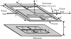
Figure 7. 3D model of dual-axis micromirror. The micromirror is suspended with the torsional beams. The electrodes  are used to tune the stiffness of the system. Reprinted from [10], copyright 2006, with permission from Elsevier.
Download figure:
Standard image High-resolution imageNano-resonators.
Nano resonators are very small MEMS devices that often operate in the order of megahertz (MHz), or even gigahertz (GHz). These devices are being applied, for example, in the field of ultra-sensitive mass sensing [30–32] and radio frequency signal processing [33]. The resonators are usually doubly clamped structures, as shown in figure 8. The resonating structure can either be a micro-fabricated beam or an even smaller structure such as a carbon nanotube or graphene flake. Some of these nano resonators also have stiffness tuning capabilities. The common tuning method for this class of devices is parallel plate tuning. But instead of having dedicated structures that cover the stiffness tuning as discussed in the previous paragraph, the resonator itself serves as tuning electrode. The substrate of the device is commonly used as the tuning electrode. Just like the devices discussed in section 3.1.1, an electrostatic (negative) stiffness can be added to the system. One device is discussed as an example for these type of devices. Other devices that use the same tuning method were reported by Schwab et al [11], Kwon et al [34], Lopez et al [35], Yan et al [36], Stiller et al [37] and Wu et al [38].
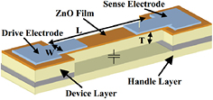
Figure 8. Voltage-tunable, piezoelectrically-transduced single crystal silicon resonators. Reprinted from [39], copyright 2004, with permission from Elsevier.
Download figure:
Standard image High-resolution imagePiazza et al [39] reported on quality factor enhancement and capacitive fine tuning of resonators. The device is intended as a high quality factor MEMS resonator for on-chip filtering and frequency reference. The resonance frequency of the device can be tuned by applying a voltage between the substrate and the device layer. The ZnO layer is a piezoelectric layer. By applying a voltage between the drive electrode and the device layer, a vibration can be induced. The vibration of the device can be sensed by measuring the voltage on the sense electrode. The configuration of the device is shown in figure 8. The untuned frequency of the device is 719 kHz and for a tuning voltage of 20 V the resonance frequency decreases with 6 kHz. There is insufficient data available to determine the stiffness of the system.
Some of these nano resonators have the capability to tune the stiffness both positively as negatively in the same device. However, the positive stiffness tuning is for the resonance mode perpendicular to the mode of the negative stiffness tuning. An electrode is placed along the side of the resonator, in the same plane. When a voltage is applied between this electrode and the resonator, a negative stiffness is added to the in-plane motion. This voltage also has the effect that the resonator is pulled into the direction of the electrode, due to the electrostatic forces. This force induces a tensile stress in the resonator. When the beam vibrates in the out-of-plane mode, this tensile stress causes a stiffening effect. This effect is explained in section 3.4. This method of both positive and negative stiffness tuning has been applied by Fung et al [40], Pandey et al [41], Rieger et al [42], Solanki et al [43], Fardindoost et al [44] and Kozinsky et al [45]. The last of these is discussed in more detail as an example.
Kozinsky et al [45] presented a device with an electrostatic mechanism to tune the nonlinearity of a resonator, increase the dynamical range and tune the resonance frequency. A theoretical model was developed that can serve as a design guideline, and a device was fabricated. This section only goes into the details of the frequency tuning capabilities. The device consists of a clamped-clamped beam with dimensions of  μm. A gate electrode is placed 400 nm from this beam and covers almost the entire length as shown in figure 9. This electrode can apply a DC bias voltage and an AC actuation voltage. The resonance frequencies of both in-plane and out-of-plane motion were measured. When the gate electrode exerts a DC voltage to the resonator, both the in-plane and out-of-plane frequencies change. Two different mechanisms are responsible for the change in stiffness. For the in-plane resonating mode the resonance frequency will decrease, because the electrostatic force will add a negative stiffness. The untuned resonance frequency of the in-plane motion is 8.78 MHz and can decrease by 6% for a tuning voltage of approximately 28 V (estimated from figure 9). This corresponds to an increase of 12% in stiffness according to equation (3). For the out of plane mode the resonance frequency will increase as a result of induced stress in the beam. The gate electrode can exert a force on the resonator, resulting in tensile stress in the beam. The untuned resonance frequency is 7.60 MHz and for a tuning voltage of approximately 30 V the resonance frequency increases by 4%. This corresponds to an increase of 8% in stiffness according to equation (3).

Figure 9. Elastic tuning of frequency upward (b) for the beam's vibration out of plane with the gate (a). Capacitive tuning of frequency downward (d) for vibration in the plane of the gate (c). The blue curve in (d) is the prediction of the theoretical model for the capacitive frequency tuning. Reprinted with permission from [45]. Copyright 2002, AIP Publishing LLC.
Download figure:
Standard image High-resolution image3.1.2. Electrostatic: varying gap.
The concepts in this section are similar to the parallel plate devices of section 3.1.1. The comb structure is commonly applied and the stiffness is added by applying a voltage between a moving and a stationary electrode. But the direction of motion is perpendicular compared to the parallel plate devices (x-direction instead of y, for figure 2). If we look at equation (7), it was shown that no electrode stiffness can be added in this direction for two flat, parallel electrodes. However, by having a gap g(x) that is a function of the displacement in x, a stiffness can be added to the system. This is illustrated in figure 10. The equation governing the stiffness can be derived as:

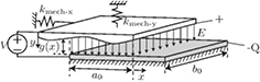
Figure 10. Two conductive plates, that have overlapping surface  , gap g(x), with a potential difference V. The charges (+Q and −Q) accumulate on the plates and form the electric field
  . The bottom plate is fixed, and the top plate can move in x and y direction.
Download figure:
Standard image High-resolution imageBecause the capacitance now is a function of the motion in x-direction, the derivative of the force term does not become zero and yield a non-zero stiffness. By tailoring the gap shape, the force-deflection relation (stiffness) can be chosen by design.
This method was applied to a number of devices. The first notion of a variable gap comb drive was in the context of actuators [46–48]. Later this was applied to stiffness tuning mechanisms. Jensen et al [14] applied the method to a comb-finger structure. Seven shapes of comb fingers were designed, of which two were fabricated and tested. The shape of the fingers was different, but applied in the same device. One of the fabricated designs has a shape such that the system becomes stiffer ((a) in table 2) under an applied voltage, the other fabricated one becomes more pliant ((b)) in table 2). The schematic drawings of the stiffening (a) and weakening (b) comb shapes can be seen in figure 11. When the gap becomes smaller for a displacement x,  is negative, resulting in a negative stiffness. The opposite applies to gaps that become larger for a displacement x. The stiffness was tuned from 0.47 N m−1 to 0 N m−1 with the weakening fingers for 80 V and to 0.75 N m−1 with the stiffening fingers for 90 V.

Figure 11. Schematic drawings of the weakening (a) and stiffening (b) comb shapes. The gap size changes with displacement x so the electrostatic force is a function of the displacement. [14].
Download figure:
Standard image High-resolution imageThe same concept was applied by Engelen et al [12], who developed a musical instrument using MEMS technology with stiffness tuning capabilities. The device consists of several similar resonators, that differ in mass and spring constant and thus (untuned) resonance frequency. Because the softest device has the largest normalized change in stiffness, this device is included in table 2 and figure 1. The theoretical stiffness is 0.6 N m−1. The resonance frequency of this device decreases approximately 5% for a tuning voltage of 29 V, so the normalized change in stiffness is 1.11 according to equation (3).
The device of Lee et al [15] applies the same method. The nominal stiffness of the device is 2.64 N m−1. By applying a tuning voltage up to 150 V, this stiffness can be decreased by 80% to 0.53 N m−1.
Varying shape electrodes were similarly applied by Guo et al [13]. The untuned stiffness is 17.3 N m−1 and the linear electrostatic stiffness is  N m−1 V−2. For a tuning voltage of 60 V this results in a change of
  N m−1.
3.1.3. Electrostatic: varying overlapping surface.
In equation (7) it was shown that it was not possible to generate a stiffness in the x-direction for flat parallel plates. In that case, the second derivative of the energy U(x) with respect to x will be equal to zero (so there is no electrostatic stiffness). But when a comb drive is designed such that the overlapping surface A has a higher order dependency on the displacement (xn with  ), the second derivative of the energy with respect to x will not be equal to zero. There will be an electrostatic stiffness in the x-direction. The equations for the capacitance, electrostatic force and stiffness yield:
So if  , there is an electrostatic stiffness in the x-direction. This non-linearly varying overlapping electrode surface can be achieved by using a comb drive with fingers of varying length. This concept was first applied by Lee et al [18]. Later, Dai et al [16], Scheibner et al [20, 49], Shmulevich et al [50] and Kao et al [17] used the same method. This type of tuning comb is shown in figures 12 and 13. The electrostatic stiffness
  as presented by Kao et al can be calculated as:
with N the number of combs,  the permittivity, th the thickness of the device, and H, b, B, p and d geometric properties that can be found in figure 12. A device with a theoretical untuned stiffness of 17 N m−1 was fabricated. Under a tuning voltage of 30 V the stiffness increased with 21% to 20.6 N m−1.
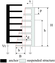
Figure 12. Tuning-comb of the tunable resonator. Reprinted from [17], used under the terms of the creative commons attribution 4.0 license.
Download figure:
Standard image High-resolution image
Figure 13. Schematic structure of the tunable resonator. Reprinted from [17], used under the terms of the creative commons attribution 4.0 license.
Download figure:
Standard image High-resolution imageScheibner et al [20, 49] used varying length comb fingers in a 'wide range tunable resonator'. The purpose of the device is to recognize the wear state in machinery, by checking the mechanical vibrations. It consists of an array of eight cells, such that a total range of 1 kHz– 10 kHz is covered. Each cell in the array has a fixed base frequency, which can be decreased by applying a tuning voltage. The tuning ranges of each subsequent cell are overlapping, so that no gap will occur in the total bandwidth. In table 2 cell one (a) and eight (b) are included as separate devices. Cell one has a theoretical untuned stiffness of 2.09 N m−1, the theoretical stiffness of cell eight is 17.59 N m−1. To approximate the tuned stiffness of the two cells the ratio between the measured tuned and theoretical untuned resonance frequencies is used (as described in equation (3)). This results in a tuned stiffness of 0.2 N m−1 and 14.7 N m−1 for cell one and eight respectively. These two extremes are included in table 2 and figure 1 as (a) and (b) respectively.
Dai et al [16] presented a similar device with a (theoretical) untuned stiffness of 0.76 N m−1. For a tuning voltage of 40 V, the stiffness drops to 0.4 N m−1. Shmulevich et al [50] achieved a broad linear range of stiffness tuning with a similar device. The stiffness of the device was not presented, but the resonance frequency was changed from 957 Hz–173 Hz for a tuning voltage of 81 V, resulting in a normalized change in stiffness of 30.6 according to equation (3). Lee et al [18], who were the first to develop this tuning method, achieved tuning from 0.3 N m−1 to 0.28 N m−1.
A different approach was chosen by Morgan et al [19]. Instead of having varying comb finger lengths, the vertical dimension of the comb fingers was varied. This is illustrated in figure 14. These structures could be manufactured due to 'gray-scale' technology, which allows the fabrication of varying height structures with a single lithography and dry etch step. Both positive and negative tuning can be achieved, by designing the combs such that the overlapping surface decreases or increases respectively. Several designs were presented and those with the largest positive (a) and negative (b) tuning range were added to table 2. The largest positive change in stiffness is from 6.1 N m−1 to 7.55 N m−1 for 120 V and the largest negative stiffness tuning was from 4.3 N m−1 to 3.3 N m−1 for 90 V.

Figure 14. Comb fingers with varying height, resulting in a changed electrostatic stiffness [19].
Download figure:
Standard image High-resolution imageA varying overlapping electrode surface was applied to a MEMS gyroscope by Hu et al [51]. A proof-mass is brought into resonance in the x-direction. The resonance frequency in the y-direction should be the same as in the x-direction, such that a rotation of the device results in a transfer of energy from the actuated resonance mode (x-direction) into the sensing direction (y-direction) due to the Coriolis effect. But due to manufacturing errors the resonance frequencies of the in-plane modes do not match. Stiffness tuning is used to change the resonance frequency in the y-direction such that it matches the frequency of the mode in the x-direction. The tuning electrodes are placed below the electrodes that are connected to the proof mass. The tuning electrodes are triangularly shaped, as shown in figure 15, such that the overlapping surface changes non-linearly when the top electrode moves in the y-direction. The stiffness is determined by the shape of the electrodes. The resonance frequency is tuned from 1.984 kHz to 2.005 kHz for a tuning voltage of 17.5 V.

Figure 15. Top view of triangular tuning electrodes as applied by Hu et al [51]. The triangular electrodes are situated below the electrode that is connected to the proof mass. By applying a voltage between the electrodes, an electrostatic stiffness can be added to the system. The shape of the triangluar electrodes influences the stiffness.
Download figure:
Standard image High-resolution imageA varying overlapping electrode surface was applied in an angular vertical comb drive by Eun et al [52]. A torsional micro mirror is suspended by two torsional springs. Perpendicular to the springs a comb structure is applied, which overlaps with stationary electrodes. When the micro mirror rotates, the overlapping surface between the moving and stationary electrodes changes non-linearly. This adds a torsional stiffness to the system. The architecture of the device can be found in figure 16. The unmodified resonance frequency of 3176 Hz was tuned to 3066 Hz for a tuning voltage of 30 V.
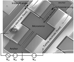
Figure 16. The microscanner consists of a rotor, two torsional springs, and two fixed electrodes. The single-crystal silicon torsional springs are plastically deformed such that the rotor including the micromirror and movable comb finger electrode has an initial tilt angle with respect to the stator electrodes. Two electrically isolated fixed electrodes including a driving electrode for actuation and a tuning electrode for tuning of the resonant frequency are symmetrically placed on both sides of the rotor with respect to the torsional springs. Reprinted from [52], used under the terms of the Creative Commons Attribution 4.0 license.
Download figure:
Standard image High-resolution image3.1.4. Electrostatic: non-interdigitated comb fingers.
The previous electrostatic tuning mechanisms of sections 3.1.1–3.1.3 were based on overlapping comb fingers. It is possible though to use non-interdigitated comb fingers for stiffness tuning. These comb fingers do not overlap and use fringe fields to exert a displacement-dependent force on each other. Due to the complexity of these fringe fields, it is not possible to derive an analytical equation for the electrostatic stiffness. Finite element modeling is needed to find this electrostatic stiffness. Both positive and negative stiffness tuning can be achieved, depending on the initial alignment of the fingers.
This method of stiffness tuning was applied by Adams et al [6, 21]. The device is shown in figure 17. For these transverse non-overlapping comb drives it is possible to have either a positive or a negative electrostatic stiffness, depending on the initial alignment of the comb fingers. When the initial alignment of the fingers is such that a moving finger is in between two stationary fingers, the restoring force will decrease with a displacement. This adds a negative stiffness to the system (denoted as (b) in table and graph). When the fingers of the stationary and moving parts are aligned, a relative motion will cause a restoring force. This is a positive electrostatic stiffness (c). Both these configurations are applied in a similar device; only the initial alignment is different. These initial configurations are illustrated in figure 18. This device has also been used by Zhang et al [53] to research nonlinearity effects on an auto-parametric amplification. The theoretical untuned stiffness of the mechanical mechanism is 2.6 N m−1. The experimental electrostatic stiffnesses are  N m−1 V−2 and
  N m−1 V−2 for the reduction and augmentation system respectively. The tuning voltage squared is estimated from figure 5 to be 3200 V−2 and 5200 V−2 respectively, resulting in a change of stiffness of
  N m−1 and 5.2 N m−1. DeMartini et al [54] applied the same tuning method for both positive and negative stiffness tuning, but insufficient data was presented to determine the change in stiffness. The device was based on earlier work of Rhoads et al [55].
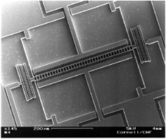
Figure 17. SEM image of a tunable resonator with a transverse(-reduction) actuator. Reproduced from [6]. © 1998 IOP Publishing.
Download figure:
Standard image High-resolution image
Figure 18. Diagram of transverse non- overlapping comb drive designs: (a) transverse reduction, (b) transverse augmentation. The lower halves are fixed in place and the upper halves are constrained to move horizontally. Reproduced from [6]. © 1998 IOP Publishing.
Download figure:
Standard image High-resolution image3.2. Mechanical
The stiffness of a system can be adjusted by mechanically changing the suspension. In MEMS this suspension usually consists of several flexural beams, that suspend parts of the chip. The stiffness of these beams is determined by the geometry, material properties and boundary conditions. The influence of the boundary conditions is shown in figures 19(a) and (b). A cantilever, clamped at one side and free at the other, is shown in figure 19(a). When the beam is clamped at both ends, the situation is as shown in figure 19(b). The stiffness is increased four times. The stiffness of a suspended system can be increased by engaging more of these flexures, or changing the effective length.
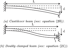
Figure 19. Beam in two configurations: cantilever and doubly clamped. The stiffness is a function of Young's modulus E, second moment of inertia I and length L.
Download figure:
Standard image High-resolution image3.2.1. Mechanical: change effective length.
Kafumbe et al [56] used the pull-in of a cantilever beam to change the effective length and tune the stiffness of the system. The configuration of the design is shown in figure 20. An electrode is placed close to a cantilever. By applying a voltage between the cantilever and electrode, the cantilever will start bending toward the electrode. This corresponds to state 1 in figure 20. At a critical point, the cantilever will snap in towards the electrode and a dielectric layer on top of the electrode prevents a short circuit. The snap in occurs when the electrostatic forces exceed the mechanical restoring forces of the cantilever. The cantilever is now in a stable clamped-pinned state (state 2). In this state the stiffness decreases for an increasing voltage. This results in a second unstable state after which the cantilever will move into the clamped-clamped configuration, which corresponds with state 3 in figure 20. If the voltage is further increased, the contact area between the cantilever and insulative layer will start to increase. This results in a change in effective length, so that the stiffness is changed. When the tuning voltage is decreased once the cantilever is snapped-in, there will be a hysteresis in the system, due to stiction between the cantilever and dielectric layer. Several mechanisms are responsible for the change in stiffness: adding electrostatic stiffness (states 1 and 2), change of boundary conditions (from state 1 to state 2 and state 2 to state 3) and change in effective length (state 3). The device has a long, linear operational range in state 3. The device is intended to work in this state. The change in normalized resonance frequency for the applied normalized voltage for the different stages is shown in figure 21.
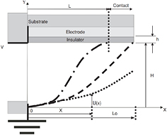
Figure 20. System configuration and states. State 1 is represented by ( ), state 2 by (- - - -) and state 3 by (— · —). Reproduced with permission from [56]. © 2005 IOP Publishing.
Download figure:
Standard image High-resolution image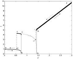
Figure 21. Normalized frequency variation with both increasing (A → B → C → D → G → Z), and decreasing normalized actuation voltage (Z → I → J → E → F → A) for the states 1 (- - - -), 2 (( ) and —) and 3 (—). Reproduced with permission from [56]. © 2005 IOP Publishing.
Download figure:
Standard image High-resolution imageAnother device that uses the principle of length change for stiffness adjustment is presented by Zalalutdinov et al [57]. A Scanning Tunneling Microscope (STM) is used to locally actuate and constrain a silicon nitride cantilever. The vertical motion of the STM is actuated by an AC voltage signal on the piezo drive, which is used to drive the cantilever. The force between the STM tip and cantilever provides an actuation and motion constraint. By changing the position where the STM tip engages the cantilever, the effective length is changed. This results in a stiffness and resonance frequency change. A change in resonance frequency of 300% is reported. The engagement of the STM tip with the cantilever can be seen for two different spots on the cantilever in figure 22. The first image (a) is actuated at the base of the cantilever, the second (b) at 45 μm from the base. The resulting change in resonance frequency can be seen in part (c) of the image. There is insufficient data provided to calculate the stiffness of this system.
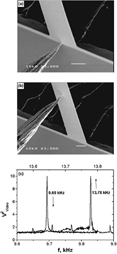
Figure 22. Scanning electron micrographs (scale bar corresponds to 10 μm) of the silicon nitride cantilever with the STM tip engaged at the base (a) and 45 μm away from the base of the cantilever (b). Plot (c) shows the corresponding resonant peaks acquired from the intensity of the secondary electrons (video signal). Reprinted with permission from [57]. Copyright 2000, AIP Publishing LLC.
Download figure:
Standard image High-resolution imageZine-El-Abidine et al [22] developed an electrostatic comb resonator with adjustable stiffness by using the change in effective length. The device is shown in figure 23. This device moves in-plane, and its position can be determined by measuring the capacitance between the moving and stationary fingers. By changing the effective length of the suspension beams the stiffness of the system changes. This change in effective length is achieved by electrostatic attraction of the suspension beams along a curved electrode as shown in figure 24. By applying a sufficiently large voltage between the electrode and the beam, the beam will be pulled in. In order to prevent a short circuit between the suspension beams and electrodes, silicon dioxide stoppers are used. These stoppers are insulated from the electrodes and will be the only contact points with the beam. There are three states in which the system can operate: zero sets activated, one set activated and two sets activated (In order to keep the system symmetrical it is only possible to actuate an entire set of actuators and not just one beam). The bias voltage that was used is 240 V. When an actuator is activated the effective length changes from 300 μm to 160 μm. The thickness of the structure is 25 μm and the width of the beams is 2 μm. Simple beams on the same die have been used to test the Young's modulus (107 GPa). The stiffness has been calculated using equation (21). The stiffness of the system in the three different configurations can be found in table 3. The maximum change in stiffness is used in table 2 and figure 1.

Figure 23. Fabricated electrostatic comb resonator with MEMS actuators with curved electrodes. Reproduced with permission from [22]. © 2009 IOP Publishing.
Download figure:
Standard image High-resolution image
Figure 24. (a) Spring state at zero voltage. (b) Spring state when the actuator is under bias. (c) Equivalent spring. Reproduced with permission from [22]. © 2009 IOP Publishing. Reproduced with permission. All rights reserved.
Download figure:
Standard image High-resolution imageTable 3. Theoretical stiffness for the different configurations (not provided in original paper.).
| Configuration | Theoretical stiffness (N m−1) |
|---|---|
| Zero bias | 3.2 |
| Two actuators | 12.0 |
| Four actuators | 20.9 |
3.2.2. Mechanically: engaging extra springs.
Mueller-Falcke et al [23, 58] proposed a mechanical way to add stiffness to a system. The application of this device is scanning probe microscopy. Usually, a cantilever is used in scanning probe applications, but instead of using a cantilever that moves out of plane, an in plane motion was used. The device has two operating modes; a soft and a stiff mode. In the soft mode, the probe is suspended by two pairs of flexure beams (flexure 1 and 3). By applying a voltage of 130 V a third pair of flexure beams (flexure 2) can be engaged, see figures 25 and 26. When these flexures are engaged, the probe is in stiff mode. The device covers an area of  μm. The proposed design has an unadjusted stiffness of 0.01 N m−1 and an adjusted stiffness of 0.1 N m−1.

Figure 25. In-plane probe design (A, electrostatic clutch; B, high aspect ratio carbon nanotube tip; C, capacitive sensor; D, comb-drive actuator). Reproduced with permission from [58]. © 2006 IOP Publishing.
Download figure:
Standard image High-resolution image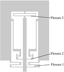
Figure 26. Plain structure of the AFM probe without sensors, actuators, tip. Reprinted with permission from [23].
Download figure:
Standard image High-resolution image3.3. Change second moment of inertia
The stiffness of a beam depends on its material properties, length, boundary conditions and cross section as shown in figures 19(a) and (b). The influence of the cross section is described with the second moment of inertia I. The general expression of the second moment of inertia for an arbitrary shape, with respect to the x-axis:
For a simple rectangular beam this is defined as:
where w and t are the width and thickness respectively. From these equations it can be concluded that a small part of surface area of  contributes more to the second moment of inertia and stiffness when it is further away from the center. Deforming the cross-section results in a change of the second moment of inertia. This results in a change in stiffness. By deforming the cross section such that the surface area moves further away from the center a stiffer system is obtained. This method is applied by Kawai et al [59]. It is applied to an atomic force microscope (AFM) cantilever, that can be used to analyze the mass of atoms and molecules. First, a surface is scanned with the cantilever in AFM mode in order to find a certain molecule or atom. This requires a stiff cantilever. When the atom or molecule is found, it is picked up with the tip of the cantilever and it is ejected in a TOF mass analyzer. But in order to reach the TOF mass analyzer, the probe must undergo a large deflection. The high stiffness of the cantilever is disadvantageous in this case, since it requires a lot of force. In order for the cantilever to switch from a soft state to a stiff state, a piezoelectric layer is used to deform the cross sectional shape, as shown in figure 27. The longitudinal piezoelectric layers are used to bend the cantilever upwards, while the transverse piezoelectric part is used to modify the cross section of the probe. By applying a voltage to the piezoelectric layer it contracts, while the underlying layer resists this contracting motion. Due to this difference in contraction, bending will occur. A schematic figure of the device and the procedure of operation can be seen in figure 27. The stiff mode is 14% more stiff than the neutral mode.
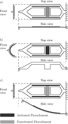
Figure 27. Schematic figure of the probe. In state (a) the probe is in its undeformed shape. In (b) the piezoelement in the center is activated and the probe deforms into a U-shape. This is the stiff mode. In (c) the probe is in soft mode and uses the two longitudinal piezo actuators on the side to bend upwards [59].
Download figure:
Standard image High-resolution image3.4. Stressing effects
The stiffness of an element is influenced by stressing effects. Either a positive or a negative change in stiffness can be achieved by applying a tensile or compressive load respectively. The effects of induced stress can be seen in the result of micro fabrication processes [60–62], due to differences in thermal expansion coefficients between subsequent layers and stresses that are inherent to the deposition processes. This is usually an unwanted effect and often the cause of failure in MEMS. Stressing effects can also be caused by adsorption of (bio-)molecules [63–69] and are used in sensing applications. These devices will not be included in this review, because the change is stiffness is not controlled, but the effect is used for sensing. Stressing effects can also be used to change the stiffness in a controlled way. The stress can for instance be applied by thermal expansion, piezoelectric effects or electrostatic loads. These methods are discussed in sections 3.4.1–3.4.3. As was already mentioned in the introduction to the review, systems that show stiffness changes due to dynamic effects will not be discussed, but might be of interest to the reader. There is a large group of devices that use non-linear dynamics for resonance frequency tuning [4, 5]. By increasing the resonance amplitude of a resonator, there will be a stiffening effect due to the increased stress. These devices will not be discussed, because this effect only occurs in a dynamic state. Nano-resonators that use both electrostatic softening and stressing effects were already discussed in section 3.1.1.
The effect of a uniform axial load on the stiffness can be understood by taking the dimensionless linear equation of motion for a beam element and dropping the damping terms and external forcing, as derived by Younis [70]. The shape of the beam is expressed by w(x, t), where x is the position along the beam and t is time:
with  (positive N means tensile force, negative means compressive), where l, N, E and I are the length, load, Young's modulus and second moment of inertia respectively. The axial load only contributes to the spatial term, which shows its influence on the stiffness. For a uniform load, a tensile force is limited by the strength of the material, while compressive load is limited by the buckling limit of the beam. When the buckling load is reached, the stiffness approaches zero.
3.4.1. Stressing effects: piezoelectric stressing.
Piezoelectric materials show mechanical deformation when an electric field is applied [71]. This deformation can be used to apply a stress to change the stiffness of a system.
Karabalin et al [72] developed a new model to predict stiffness changes in micro- and nanocantilever beams due to surface stress. The validity of this model has been confirmed with measurements. The device is a single chip with series of both cantilevers with a free end and doubly clamped beams as shown in figure 28. All have the same width of 900 nm and have the same stack of materials: 20 nm aluminum nitride, 100 nm molybdenum, 100 nm aluminum nitride, and 100 nm molybdenum. The lengths are 6, 8 and 10 μm. A voltage is applied between the molybdenum layers, such that the aluminum nitride layer will apply a stress to the stack due to its piezoelectric properties. Both a compressive and a tensile stress can be applied. This stress causes the beam to bend, because it is applied above the neutral axis of the stack. An AC voltage to the same piezo stack is used for actuation. Interferometric measurements are used to detect the resonance frequency. In table 2 only the 10 μm doubly clamped beam is included, as two separate devices; one for positive tuning voltage (a) and one for negative tuning voltage (b). Similar experiments, with an off-center piezoelectric stack on a silicon nitride doubly clamped beam were done by Olivares et al [73].

Figure 28. Resonant response of piezoelectric beams. (a) SEM micrograph of the doubly clamped beams used for the experiments. On top of the micrograph, we show resonant responses of each of the beams, yielding resonant frequencies of 38.3 MHz (length 6 μm, purple), 22.9 MHz (8 μm, green) and 14.8 MHz (10 μm, blue). Experimental details are provided in the supplementary material of [72]. (b), SEM micrograph of the cantilever beams used for the experiments. Respective resonant responses are also shown for each cantilever, yielding natural frequencies of 8.85 MHz (length 6 μm), 4.82 MHz (8 μm), 3.16 MHz (10 μm). Both types of beams have the same composition (320 nm of total thickness) and width (900 nm). Lengths are 6, 8, or 10 μm for both types of devices, causing the boundary conditions to be the only difference, thus allowing proper comparison of the experimental results for the two configurations. Scale bars: 2 μm. Reprinted with permission from [72]. Copyright 2012 by the American Physical Society.
Download figure:
Standard image High-resolution image3.4.2. Stressing effect: thermal expansion.
Most materials expand when the temperature is increased. This is a result of the increase in kinetic energy in the molecules. When a doubly clamped beam is subjected to an increase in temperature, the expansion of the material will lead to an increased internal stress, which can be used for stiffness tuning.
Two devices that made use of stressing effects by thermal expansion were presented by Syms et al [24]. A one degree- (figure 29) and two degree of freedom device were made. The first device is explained in more detail. A mass is suspended by folded flexures and is tunable in the y-direction. This is done by applying a DC-voltage between the anchors of the flexures such that a current will start to flow. Due to Joule heating, these flexures will heat up. Whether compressive or tensile stress will arise depends on the ambient pressure. This is a result of the dominant cooling mechanism; under high pressure this is convection, while thermal conduction dominates at low pressures. When the cooling is dominated by convection, the temperature will be higher in the flexures than in the suspended part, because the surface of the latter is much greater, which results in a faster cooling. The thermal expansion will be larger in the flexures than in the suspended part, so compressive stress will arise. When the pressure is low, the convective cooling will be negligible and conduction to the bulk of the chip will be the dominant cooling mechanism. The flexures and the suspended parts will have the same uniform temperature in steady state. Now the thermal expansion of the suspended part will be larger, since it is longer than the flexures; the flexures will be under tensile stress. For a compressive stress, the stiffness will decrease, while a tensile stress will result in an increased stiffness. The unadjusted stiffness of the device is not mentioned in the paper, but can be derived from the geometry. The stiffness for such a set of doubly clamped beams is shown in equation (21). Assuming that the silicon has a Young's modulus of 169 GPa [74], this results in a stiffness of  N m−1. For the lowest pressure of 10 mTorr, the increase in resonance frequency is almost 50%, resulting in 0.45 N m−1. For the highest pressure of 500 mTorr, the decrease in resonance frequency is almost 10%, resulting in 0.16 N m−1. In table 2 the device is shown as two separate devices; one for the increase in stiffness(a), the other for the decrease in stiffness (b). The two degree of freedom device has a different flexure geometry. The mass is suspended by two sets of beams instead of one and the length of the beams is smaller compared to the other device. By using equation (21) we get
  N m−1. The resonance frequency in the y-direction changes from 1.56 kHz to 2.29 kHz for 3 mW of tuning power. By applying equation (3), a tuned stiffness of 1.49 N m−1 is found. This device can be found in table 2 as device (c).
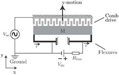
Figure 29. Schematic drawing of device with one degree of freedom. The mass is suspended by the folded flexures. A DC voltage can be applied to the flexures, and due to Joule heating the beams will heat up and expand. Depending on the surrounding air pressure, convective or conductive cooling will be dominant. For conductive cooling, the flexures will be subjected to tensile stress, because the mass expands more than the flexures. For convective cooling the flexures will expand more than the mass, resulting in a compressive stress. Compressive stress decreases the stiffness, tensile stress increases the stiffness. The AC voltage is used to actuate the device. [24]
Download figure:
Standard image High-resolution imageThe stiffness of the device designed by Remtema et al [75] is tuned by thermally induced stressing effects. The configuration of the device can be seen in figure 30. A mass is suspended by 'beam 1' and by a folded flexure mechanism that consists of 'beam 2' and 'beam 3'. The folded flexure mechanism results in a high stiffness in the x direction and a low (linear) stiffness in the w direction. By applying a current to the suspension beams, the temperature will increase due to Joule heating and the beams will expand. The expansion of 'beam 2' and 'beam 3' is in opposite directions, so no compressive stress is developed. 'Beam 1' however, will be stressed due to the thermal expansion. This stress results in the change in stiffness. On top of the stressing effect there is a second mechanism that decreases the stiffness of the structure. The Young's modulus of silicon has a negative temperature dependency, as described in section 3.5; by increasing the temperature in the suspension beams both the compressive stress as the decrease in Young's modulus will decrease the stiffness. (Because the compressive stress has the dominant effect, the device is placed in this category). The results of the change in resonance frequency of the device can be seen in figure 31. The maximum change in frequency is 14%, so according to equation (3), this is an increase of 30% in stiffness.
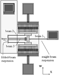
Figure 30. Schematic diagram of a comb-shape micro resonator with a straight-beam for active frequency tuning via localized stressing effects. Reprinted from [75], copyright 2001, with permission from Elsevier.
Download figure:
Standard image High-resolution image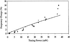
Figure 31. Measured frequency change versus tuning power for five different devices compared to the theoretical model. Reprinted from [75], copyright 2001, with permission from Elsevier.
Download figure:
Standard image High-resolution imagePreviously discussed devices use uniform heating and uniformly thermal expansion by using the suspension beam itself as the heater. This requires an electrically conductive suspension beam. Sviličić et al [76, 77] and Mastropaolo et al [78] used non-uniform thermal expansion, by using a separate electro-thermal electrode on top of the structural element that supplies the thermal energy. So thermally induced stress can also be applied to non-conductive material. This method has been applied to a doubly clamped beam [76], a cantilever beam [77–81] and a disk [78]. In the case of a cantilever beam, the expansion is not fully restricted. The thermal stress is induced due to the difference in thermal expansion coefficient between the electrode and the support material. This results in a stress gradient and out-of-plane bending of the structure.
Thermally induced stressing effects have also been applied on nano resonators. Jun et al [82] used 12 μm long doubly clamped composite beams consisting of 30 nm 3C-SiC and 30–195 nm aluminum. A current was applied to the resonator itself, resulting in Joule heating and thermally induced stress. Mei et al [83] used carbon nanotubes in similar experiments.
3.4.3. Stressing effect: electrostatic force.
Cabuz et al [84] presented a MEMS resonator of which the stiffness can be tuned by using stressing effects. This stress is applied by using electrostatic attraction. A silicon structure with a thin, doubly clamped cantilever resonator is installed in a glass package, as shown in figure 32. One of the sides of the structure is clamped in, the other side is suspended by a torsion bar. Electrodes are situated close to the top and bottom of the free hanging part of the silicon structure. These electrodes can exert a force on the structure, such that the structure can rotate around the torsion bar. An axial force will be induced to the resonator. A third electrode is placed close to the resonator to detect the deflection of the resonator by capacitive measurement. The applied voltage attracts the bottom of the free end. This induces a tensile stress in the resonator, resulting in an increase of resonance frequency. For 15 V the frequency increased with 14.5 Hz. Tuning with the upper electrode is not demonstrated, but a similar change in frequency, in opposite direction may be expected. The untuned resonance frequency is not mentioned in the paper. Yao et al [27] mentioned the use of electrostatic actuators for applying an axial force for stiffness tuning. No experimental data was provided though.
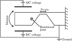
Figure 32. Schematic of device [84].
Download figure:
Standard image High-resolution image3.5. Change Young's modulus
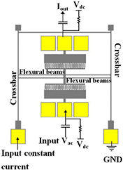
The stiffness of a mechanical structure depends on the geometry, configuration and Young's modulus (elasticity of a material). Zhang et al [85, 86] designed a device of which the stiffness can be changed by tuning the Young's modulus. A mass is suspended by four flexural beams that are connected to a crossbars as shown in figure 33. By applying a voltage to the electrodes of the device, a current will run through the crossbars and flexural beams. The flexural beams will heat up, due to Joule heating. The beams will expand, but this will not result in an axial stress, because the motion is not restricted due to the compliance of the crossbars. The flexural beams are made out of silicon, which has a negative temperature coefficient of modulus. The increase in temperature will therefore lead to a decrease in Young's modulus, and thus stiffness as shown in equations (20)–(21). Two sets of comb drives are attached to the mass. One of these comb drives is used to actuate the mass, the other is used to measure the motion. The untuned mechanical stiffness can be calculated using equation (21). For flexural beams with a size of ( )
)  μm and a Young's modulus at room temperature of 169 GPa, which gives k0 = 84.1 N m−1. For an input of 54 mW the resonance frequency drops 1.1%. According to equation (3) this means that the tuned stiffness is 97.8% of the untuned stiffness. The tuned stiffness is 82.25 N m−1. Devices that use thermally induced axial stress (section 3.4.2) usually have this effect of change in Young's modulus as well. But the effect on the change in stiffness is stronger for stressing effects than for the change in Young's modulus.
Figure 33. Schematic of MEMS resonator with integral crossbar heaters including biasing configuration used. Reprinted from [85], copyright 2012, with permission from Elsevier.
Download figure:
Standard image High-resolution image
4. Discussion
The results will be discussed for each physical principle. They are compared in table 4.
Table 4. Comparison of the categories.
| Category | Sub-category | Stiffness adjustment | Advantages | Disadvantages | |||
|---|---|---|---|---|---|---|---|
| Positive | Negative | Continuous | Discrete | ||||
| Electrostatic | Parallel plate | × | ✓ | ✓ | × | Simple, effective | Risk of pull-in, relative large tuning mechanism |
| Varying gap | ✓ | ✓ | ✓ | × | Freedom of design | Risk of pull-in, relative large tuning mechanism | |
| Varying surface | ✓ | ✓ | ✓ | × | Freedom of design | Risk of pull-in, relative large tuning mechanism | |
| Non-interdigitated | ✓ | ✓ | ✓ | × | Low risk of colliding electrodes | Complex design, less efficient, relative large tuning mechanism | |
| Mechanical | Effective length | × | × | ✓ | ✓ | Large tuning range | Mechanical contact and high voltage required |
| Mechanical springs | × | × | × | ✓ | Large tuning range | Mechanical contact and high voltage required | |
| Second moment of inertia | ✓ | × | ✓ | × | Size efficient solution, applicable to cantilever | ||
| Stressing effects | Piezoelectric | ✓ | ✓ | ✓ | × | Positive and negative tuning in same device, applicable to cantilever, size efficient | |
| Thermal | ✓ | ✓ | ✓ | × | Easily applicable, size efficient | Only small changes in stiffness | |
| Electrostatic | ✓ | ✓ | ✓ | × | Relatively large | ||
| Young's modulus | × | ✓ | ✓ | × | Relatively easily applicable | Only small changes in stiffness | |
4.1. Electrostatic
Electrostatic tuning is the most-used method for stiffness tuning. It is very versatile; almost all ranges of stiffness can be achieved. But this all comes at a cost of size. The change in stiffness is directly related to the surface area of the electrodes. So in order to achieve large changes in stiffness, a large device is needed. The simplest method of electrostatic stiffness tuning is by using the 'parallel plate' type (section 3.1.1). The range of motion of this device is limited by the risk of pull-in. This range can be extended by using branched fingers instead of straight ones. The risk of pull-in remains, though, and precautions like safety pins or other mechanical stoppers are required to ensure a long lifetime [9].
The 'varying gap' and 'varying overlapping electrode surface' have more freedom of design than the 'parallel plate' devices. The voltage-stiffness relation can be designed by choosing the rate of change in gap or overlapping electrode surface. This might enhance the performance.
Non-interdigitated comb fingers are less efficient than the other electrostatic tuning methods. The advantage is that the risk of colliding comb fingers is low, because they are not overlapping.
4.2. Mechanical
Mechanical tuning is an effective way of achieving large changes in stiffness for a limited device size. These devices are often discrete. This might be a limiting factor for certain applications. But when continuous stiffness tuning is not needed and a large change in stiffness is required, mechanical stiffness adjustment is a suitable method. Mechanical contact was found in all these methods, which could lead to stiction and wear problems. Most of the devices that use mechanical tuning use electrostatic pull-in to establish the mechanical contact, which requires a high voltage.
4.3. Second moment of inertia
The second moment of inertia describes the influence of the cross section on the stiffness of an element. By deforming the cross section, the stiffness can be changed. There is only one device in this category in this review. It uses piezoelectric elements to control the cross-sectional curvature of a cantilever. Not many tuning methods are applicable to cantilevers. The piezo actuator is very small because it is integrated in the structure. Therefore it is a size efficient solution.
4.4. Stressing effects
Stressing effects can be applied by either piezoelectric elements, thermal expansion or electrostatic forces. The piezoelectric devices can tune the stiffness both positively and negatively in a single device, because both tensile and compressive stresses can be developed, depending on the direction of the electric field. For this reason it is a versatile method. Thermal stressing can also be used to tune both in the positive and negative direction, but this can not be done in the same device under constant conditions. When the thermal expansion of the suspension element is larger than the surrounding structure, the stress will be compressive. When the expansion of the suspension is lower than the surrounding structure, tensile stress will be present. Inducing stress through electrostatic forces can also be used for positive and negative stiffness tuning, depending on the actuation direction of the actuator. The tuning range of devices in this category is relatively small.
4.5. Young's modulus
The Young's modulus is the elasticity of a material, which influences the stiffness. The Young's modulus is depending on the temperature, so it can be tuned by controlling the temperature. The Young's modulus of silicon, which is widely used for MEMS, has a negative temperature dependency. However, the effect is weak and only small changes in stiffness can be achieved because the tuning is limited by the melting temperature. This tuning method is easily applicable, because a heater is the only additional part that is needed. Devices using thermal expansion for stressing effects also show stiffness change due to a change in the Young's modulus, but this effect is much stronger.
5. Conclusion
Stiffness adjustment is broadly applied in MEMS and the applications and physical principles are numerous. The results in this paper can be used as a selection tool for the reader to find a suitable concept for a new application. The categorization as it stands now can successfully map the current state of the art, and can be extended with extra categories or sub-categories as the field develops. The field of stiffness tuning is dominated by electrostatic methods and most of the applications can be found in resonating structures like accelerometers, energy harvesters and mechanical filters.
If a large tuning range is required (more than one order of magnitude), electrostatic tuning or mechanical tuning are the most suitable methods. Electrostatic tuning requires a large device though, and mechanical tuning is often in discrete steps and requires a large tuning voltage. If a small tuning range (up to one order of magnitude) is required electrostatic tuning, stressing effects, change in second moment of inertia or tuning of the Young's modulus could be a suitable method. Table 2 provides an overview of the different devices and their key properties. Figure 1 provides a graphical overview of the devices and their absolute and normalized change in stiffness. The different categories are compared in table 4. These graph and tables serve as a selection tool for stiffness tuning.