
Abstract
This paper demonstrates the effectiveness of certain structural health monitoring (SHM) strategies based on propagation of guided elastic waves within thin-walled shell structures. This is realized based on results of numerical and experimental investigations obtained by the use of the spectral finite element method (SFEM) together with laser scanning vibrometry (LSV) and subsequent application of two different integral-based indices for damage quantification, these being the integral mean value (IMV) and the root mean square (RMS). Numerical tests by SFEM were carried out for a square plate with through-hole damage, a cracked fuselage section with two stiffeners and a cracked wing section skin, all made out of aluminium. Experimental measurements by LSV included tests on a square aluminium plate, composite plate and a composite stabilizer of a PZL W-3A helicopter, all with simulated damage. During numerical and experimental investigations damage sensitivity of both IMV and RMS indices was tested by considering various displacement components, signal timescales or weighting factors. A certain practical method for quick construction of RMS damage maps based on experimental measurements by LSV was also presented.
Export citation and abstract BibTeX RIS
1. Introduction
Lamb waves [1] are a type of elastic waves that propagate between two parallel surfaces. At certain conditions they may propagate over relatively long distances with small amplitude decrease and for this reason Lamb waves are very attractive for many engineering applications. Various anomalies in wave propagation patterns resulting from wave–damage interaction can be observed, interpreted and next employed for damage assessment [2–5]. It is well known that the presence of damage results in reflection and scattering of propagating elastic waves and such features are commonly used for damage detection and localization purposes. The results of numerical and experimental investigations presented in this work are selected in order to demonstrate the application and effectiveness of the guided elastic wave approach for that task. The so-called inverse problem associated with damage detection and localization based on anomalies in wave propagation patterns observed was solved both numerically and experimentally.
In the case of numerical simulations the spectral finite element method (SFEM), as proposed by Patera [6], was applied. As a very effective numerical tool the SFEM can be successfully employed to analyse various transient dynamic problems or high frequency dynamic responses of structures of complex geometries including propagation of guided elastic waves. This approach has its origin in the application of spectral Fourier or Chebyshev series for solutions of partial differential equations, as shown in [7]. The SFEM is based on the same ideas as the finite element method (FEM) and the main fields of its application cover fluid dynamics [8], heat transfer [9], acoustics [10], seismology [11] and also mechanical engineering [12–17].
The experimental investigations were carried out by laser scanning vibrometry (LSV). Contrary to most wave-propagation-based measurement strategies, based on the employment of PZT transducer networks [18–20] attached to or integrated within hosting structures and introducing undesired changes in the local stiffness and mass distributions that can significantly influence measurement conditions, the LSV technique is free of these issues. Moreover, as a very robust experimental technique recently the LSV has often been used for investigations of problems associated with wave propagation in various structural members. Results on propagation of Lamb waves generated in a duralumin plate immersed in water are shown in [21], while similar results on propagation of Lamb waves in an aluminium plate carried out not only numerically but also experimentally by LSV can be found in [22]. Results of this research showed that visualization of propagating waves in a damaged region led to the conclusion that the effectiveness of damage detection strongly depends on the defect size. Similar results of experimental measurements in aluminium plates by LSV for damage detection purposes by Lamb waves were presented in [23, 24], where the surface around the damage was carefully scanned. The application of a 1D version of LSV reported in [25] for measurements of Lamb waves in an aluminium plate. This work highlights the effectiveness of LSV in separation of the in-plane S0 and the out-of-plane A0 Lamb wave modes that can be utilized for damage detection purposes. The application of Lamb waves for damage detection in composite plates was successfully demonstrated in [26], confirming that this approach can be used for delamination detection and localization as well as the assessment of delamination size.
This paper presents selected results of numerical and experimental investigations by the SFEM and LSV carried out by the authors and related with propagation of guided elastic waves in plate- and shell-type structures. The application of two different integral-based indices for damage quantification is described in this paper, these being the integral mean value (IMV) and the root mean square (RMS). Both flat 2D isotropic and composite plates and 3D wing section and helicopter stabilizer were investigated. The influence of damage on the values of the two damage indices was studied in order to identify and locate precisely any damage-related discontinuities simulated during numerical and experimental tests.
2. Spectral finite element method
2.1. Element formulation
The coordinates ξi and ηj of a two-dimensional spectral finite element in the element normalized coordinate system ξη can be expressed as the roots of a polynomial equation of the following form [27, 28]:
where Pn(x) is the nth-order Legendre polynomial and the symbol ' denotes its first derivative in respect of x. In the case of the spectral shell finite element used by the authors the nodal coordinates of the element for n = 5 can be specified as:
where i,j = 1,2,...,n + 1.
On the specified nodes a set of shape functions can be built in the local coordinate system ξη. A Lagrange interpolation function f(ξ,η) supported on the nodes ξi and ηj can be defined in the following manner:
where Ni(ξ) and Nj(η) are one-dimensional shape functions of the element, while fij represent the nodal values of the function f(ξ,η). It should be emphasized that one-dimensional approximation functions Ni(ξ) are orthogonal in a discrete sense:

where wi is the well-known Gauss–Lobatto–Legendre (GLL) weight and δij is the Kronecker delta [29, 30].
Assuming small strains the displacement field within the mid-plane of the spectral shell finite element, in the local coordinate system x'y'z', can be expressed in the form presented in [27] as:
where the displacement components u0(x',y'), v0(x',y') and w0(x',y') can be interpreted as the averages of the displacements measured at the upper and lower surfaces of the element. At the same time the displacement components Φ(x',y'), Ψ(x',y') and Ω(x',y') can be thought of as about the differences between those upper and lower surface displacements related to the element thickness h. Relations between the upper and lower surface displacements and the displacement components in the current formulation of the spectral shell finite element can be expressed as:
It should be noted at this point that the number of independent displacement components in (5) is directly linked with the number of wave modes that can be considered by the use of the spectral shell finite element, as shown below.
Following the notation used in [29] and under the assumption of small strains and by taking into account the form of the displacement field expressed by (5) the strain field within the element in the local coordinate system x'y'z', according to the first-order shear deformation theory, can be calculated based on the following relations [29, 30]:
leading to the definition of the characteristic inertia (diagonal) and stiffness matrices of the spectral element in the local coordinate system x'y'z', as shown in [27].
It can be clearly seen from equation (7) that in the current formulation of the spectral shell finite element the additional displacement component Ω(x',y') denotes, in fact, the  z' strain component vital for the element performance as well as its capability of modelling simultaneously the symmetric and antisymmetric dynamic behaviour associated with the propagation of elastic waves.
2.2. Dispersion curves
The effectiveness and correctness of a particular shell theory in modelling various dynamic or wave-propagation-related problems by the SFEM can be easily evaluated and assessed by analysing the dispersion curves associated with these theories. Moreover the dispersion curves give a great insight into the performance of spectral finite elements under various conditions and allow one to estimate the applicability of the elements by comparison of numerical results with known analytical results.
Dispersion curves can be calculated in two straightforward steps. Firstly it is necessary to determine equations of motion associated with the theory under investigation. This can be easily achieved by the use of Hamilton's principle. Next, based on the given displacement field the virtual work W related to deformation and motion of a spectral finite element is expressed in terms of its strain energy U and kinetic energy T as well as the work of some external forces F. Subsequent application of Hamilton's principle leads to a set of equations of motion that are derived for each component of the displacement field.
Secondly, propagation of harmonic waves is assumed, which helps to transform the equations of motion from a set of partial differential equations, defined in the time domain for each displacement component, into a set of linear homogeneous equations defined in the frequency domain for the amplitudes of each displacement component. This system can be solved only then when its determinant vanishes, which gives rise to the characteristic polynomial equation. The roots of this equation define dispersion relations between particular modes of harmonic waves that are allowed to propagate by the theory investigated, the wavenumber k and the angular frequency ω as well as the dispersion curves for the phase cp and group cg velocities, as shown in figure 1, where cl and ct denote the velocities of longitudinal (irrotational, voluminal, dilatational or primary) and torsional (rotational, equi-voluminal, shear or secondary) waves propagating in three-dimensional unbounded isotropic media, respectively [31, 35]. The values cl = 6.3 km s−1 and ct = 3.2 km s−1 correspond to aluminium alloy 2024-T3. The computational procedure described above and applied by the authors is based on the procedure presented in [31], which is also described in detail in [34].
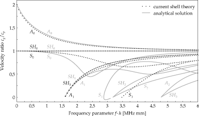
Figure 1. Dispersion curves for the group-to-phase velocity ratio for the shell theory under investigation (cl = 6.3 km s−1 and ct = 3.2 km s−1).
Download figure:
Standard imageIn the present case the spectral shell finite element under consideration was assessed in terms of its accuracy expressed by the relative error δ of the group-to-phase velocity ratio cg/cp, obtained based on the displacement field given by (5), and the same velocity ratio calculated analytically based on the Lamb solutions [1].
The relative error δ is defined as follows:
where T denotes the group-to-phase velocity ratio cg/cp obtained for the given shell theory, while L denotes the same ratio obtained for the Lamb solutions [1]. Furthermore, in order to estimate a broad frequency accuracy of the theory an average error Δ can be defined in the following manner:
The obtained results are presented in figure 2 for the fundamental symmetric S0, antisymmetric A0 and shear symmetric SH0 wave propagation modes. It should be noted that the relative error δ is a function of not only the frequency f but also the thickness of the element h. In the case of the symmetric wave mode S0 the error is positive and increases gradually with an increase in the frequency parameter fh. It is equal to 1.47% for 1 MHz mm, while its value reaches 34.1% for 2 MHz mm. In the case of the antisymmetric wave mode A0 the error stays small and negative in the whole range of the frequency parameter fh. It is equal to −1.56% for 1 MHz mm and has a local minimum equal to −1.6% for 1.35 MHz mm. It is interesting to note that within the whole range of the frequency parameter fh the value of the relative error δ for the fundamental shear symmetric wave mode SH0 is equal to zero. The corresponding values of the average error Δ calculated up to 1 MHz mm and 2 MHz mm are equal to 0.39% and 5.41% for the symmetric wave mode S0 and 1.01% and 1.29% for the antisymmetric wave mode A0.
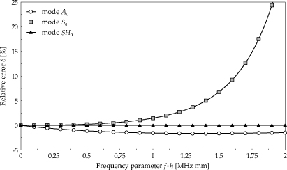
Figure 2. Relative error δ as a function of frequency parameter fh calculated for the fundamental symmetric S0, antisymmetric A0 and shear symmetric SH0 wave propagation modes for the shell theory under investigation (cl = 6.3 km s−1 and ct = 3.2 km s−1).
Download figure:
Standard imageBased on the results shown in figure 2 it can be concluded that the practical range of application of the shell theory under consideration is limited by the cutoff frequency of the antisymmetric A1 and shear antisymmetric SH1 wave modes, as presented in figure 1. This is approximately equal to 1.6 MHz mm. Within this range of the frequency parameter fh numerical results are characterized by small errors and stay close to the analytical solutions. However above 1.6 MHz mm the errors increase significantly due to the inability of the current theory to reproduce the appropriately complex multimode behaviour observed.
3. Numerical simulations
Numerical simulations were divided into two parts. In the first part a flat 2D square plate was investigated, while in the second two 3D shell structures were analysed, i.e. a fuselage section with two stiffeners and a wing section skin. It was assumed that the structures were made out of aluminium alloy 2024-T3 with the following material properties: elastic modulus E = 72.7 GPa, Poisson's ratio ν = 0.3, mass density ρ = 2700 kg m−3 and 10 mm of thickness.
In all three cases propagation of guided elastic waves was simulated and investigated by SFEM and the spectral shell finite element presented and discussed earlier. Changes in wave propagation patterns were carefully studied in the context of damage detection and localization [36–39]. As a source of excitation a 75 kHz four-cycle sine pulse modulated by the Hann window was employed. The structures under consideration were modelled by approximately 2500 shell spectral finite elements, while the total numbers of model degrees of freedom were approximately equal to 380 000. Boundary conditions of free type were considered, while the time of numerical simulations covered 0.4 ms divided into 8000 equal time steps in each case.
Based on the wave propagation patters certain damage-related maps can be easily constructed [36–39]. However, in order to overcome the problems resulting from the presence of dead zones (i.e. such zones in which damage cannot be detected by classical methods), as presented in [36–38], it was decided to employ a different approach. In this approach damage-related maps were based on two different time integral indices calculated at selected points of the structures, these being the integral mean value (IMV) and the root mean square (RMS).
For a time signal s(t) sampled at n points with time intervals Δt the following relation can be written:
where t1 and t2 denote the beginning and the end of the sampling process, based on which the IMV and RMS time integral indices may be defined as follows:
The RMS time integral index (12) can be further modified by adding a weighting factor w(t), which decreases the importance of the time samples closer to the beginning of the sampling process and increases the importance of the samples closer to its end. This can be easily achieved by the following simple modification:
where

It can be noticed that for the weighting factor wk = k (m = 1) the importance (weight) of particular time samples increases linearly with time t, while when the weighting factor wk = k2 (m = 2) this importance (weight) increases as a square function of time t.
In practice, the approach proposed above can be successfully realized by LSV. However, in the current numerical study as measurement points used to calculate the values of the integrals (12)–(14), selected elemental nodes were taken in which all displacement components were calculated. Based on them the IMV and RMS damage maps were calculated at various time instances in order to reveal the influence of wave–damage interactions, reflections as well as mode conversion.
3.1. 2D case of a flat aluminium plate
For the square aluminium plate shown in figure 3 the IMV and RMS damage maps obtained and based on the results of numerical simulations are presented in figures 4 and 5. They were calculated for a force excitation of 1 N acting transversely at the top surface of the plate and at the plate centre. The maps were plotted for all three displacement components u, v and w and as damage a through hole of 10 mm diameter was assumed.
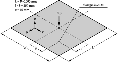
Figure 3. Geometry of a flat aluminium plate with a through hole.
Download figure:
Standard image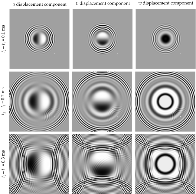
Figure 4. Evolution of IMV damage maps in time based on results of numerical simulation by the SFEM for the case of 2024-T3 aluminium plate with through-hole damage (t1 = 0 ms).
Download figure:
Standard image
Figure 5. Evolution of RMS damage maps in time based on results of numerical simulation by the SFEM for the case of a 2024-T3 aluminium plate with through-hole damage (t1 = 0 ms, wk = 1).
Download figure:
Standard imageIt can be seen from the results presented in figures 4 and 5 that both the IMV and RMS damage maps can indicate well the location of the through-hole damage. This is true for all displacement components investigated. However, in the case of the RMS damage map the position of the damage is more clearly visible if only the sampling time interval Δt is long enough for the propagating waves to reach the damage. It is interesting to note that the use of the in-plane displacement components u and v results in good sensitivity in both cases. However, from a practical point of view measurements of the out-of-plane displacement components by LSV is much easier due to their higher values and signal-to-noise ratios. Because of that only the transverse displacement component w was taken into consideration in all the following results presented.
The results of numerical simulations presented in figure 6 show the influence of the weighting factor wk used for generation of RMS damage maps on the effectiveness of damage detection and localization in the plate under investigation. In the case of unweighted RMS damage maps (wk = 1) the position of the through-hole damage is visible for all displacement components u, v and w, but the patterns observed are strongly dominated by the excitation source located at the plate centre. In certain cases this effect can be dominating and too strong to allow one to pinpoint any damage. This undesired behaviour can be avoided when linearly weighted RMS damage maps are used (wk = k), while square weighted RMS damage maps (wk = k2) offer further improvement. However, it should be pointed out at this place that the use of weighted RMS damage maps requires appropriately chosen sampling time intervals Δt in order to minimize the influence of the boundary reflected waves that can mask any effects originating from the damage.
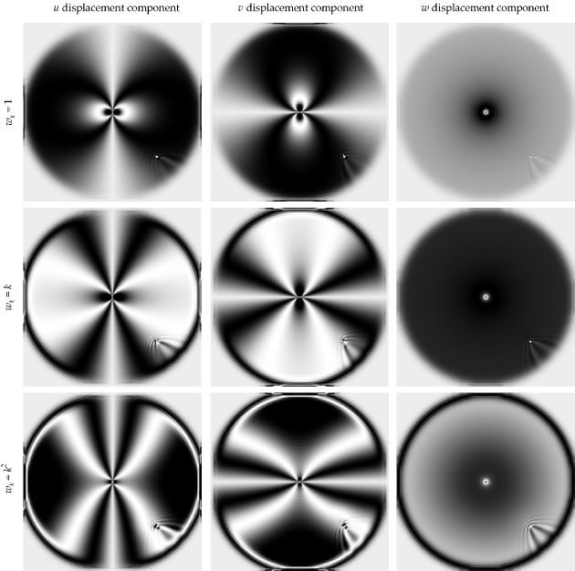
Figure 6. The influence of weighting factors wk on RMS damage maps based on results of numerical simulation by the SFEM for the case of a 2024-T3 aluminium plate with through-hole damage (t1 = 0 ms, t2 − t1 = 0.2 ms).
Download figure:
Standard imageIt should be noticed that, due to the 2D nature of the plate, the IMV and RMS damage maps are virtually based on the behaviour of the fundamental antisymmetric A0 wave propagation mode only that is dominating in the current case. For that reason it is visible from the RMS damage maps that the transverse displacement component w is more sensitive to the weighting process, while the in-plane displacement components u and v indicate smaller sensitivity to it.
Contrary to the previous case of the 2D plate the following two numerical examples are concerned with 3D shell structures. Their 3D geometry results in a much more complex nature of their responses and because of that in these two cases the RMS damage maps were based on the amplitude  of the total displacement rather than each particular displacement components u, v and w.
3.2. 3D case of cracked shell structures
Next two numerical cases are concerned with a cracked fuselage section with two stiffeners, as presented in figure 7, and a cracked wing section skin, shown in figure 8. It was assumed that both these structures are damaged and the damage has the form of an open crack of 10 mm length located on the circumference of the inner opening (window hole) of the fuselage section or is located on the leading edge of the wing section skin. The crack was modelled using a technique developed by the authors in the past for various applications of the finite element method (FEM), an approach described in details in [40–42]. The stiffness loss due to the crack was calculated according to the laws of fracture mechanics.

Figure 7. Geometry of a cracked fuselage section with two stiffeners.
Download figure:
Standard image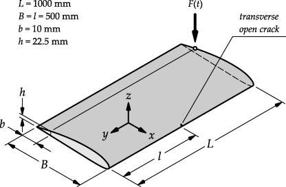
Figure 8. Geometry of a cracked wing section skin.
Download figure:
Standard imageThe results of numerical simulations corresponding to both analysed cases presented in figures 9 and 10 refer to the linearly weighted RMS damage maps (wk = k) and their evolution in time. It can be clearly seen from the results of numerical simulations presented in figures 9 and 10 that the patterns observed originate from a complex interaction and conversion between the symmetric S0 and SH0 and the antisymmetric A0 wave propagation modes in both cases. Despite their complexity it should be strongly emphasized that, as soon as propagating waves fully reach the crack position, which best corresponds to the time intervals t2 − t1 = 0.3 ms and t2 − t1 = 0.4, the crack location and orientation become very well visible.
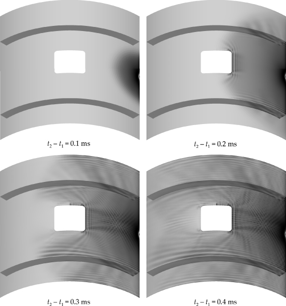
Figure 9. Evolution of RMS damage maps in time based on results of numerical simulation by the SFEM for the case of a cracked fuselage section with two stiffeners (t1 = 0 ms, wk = 1).
Download figure:
Standard image
Figure 10. Evolution of RMS damage maps in time based on results of numerical simulation by the SFEM for the case of a cracked wing section (t1 = 0 ms, wk = 1).
Download figure:
Standard image4. Experimental investigation
In order to verify the proposed method a wide programme of experimental measurements was carried out by the use of LSV. This programme included tests on selected thin-walled structures with simulated damage. During the tests damage sensitivity of both IMV and RMS indices was assessed.
A general view of the unit is presented in figure 11. Its most important part is a sensor head with laser Doppler vibrometer that enables one to perform fast, accurate and non-contact measurements of vibration velocities of whole surfaces. Thanks to this many undesirable effects that could possibly distort the results of measurements can be avoided. Its main advantages come from automatic, high sensitivity and non-contact measurement capabilities during which entire surfaces can be rapidly scanned and automatically probed with flexible and interactively created measurement grids. The LSV unit automatically moves to each point on a scanning grid measuring responses and validates each measurement by checking the signal-to-noise ratio.
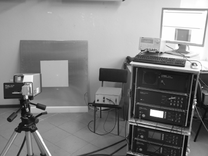
Figure 11. Polytec PSV-400 laser scanning vibrometry unit used for experimental measurements.
Download figure:
Standard imageIn order to provide optimal conditions during measurements any dispersion of the laser beam reflected from a measurement surface should be avoided. A small amount of light returning to sensor heads would result in relatively low signal-to-noise ratios. In order to overcome this effect the measured area was taped with a special reflective foil of such a property that it always reflects light off in the source direction. The measurements were carried out for two types of thin plates (aluminium and composite) with the dimensions of 1000 mm × 1000 mm as well as for the composite stabilizer of a PZL W-3A helicopter. Due to the geometry of the objects only the transverse displacement components were taken into account during all experimental measurements.
4.1. Aluminium plate
The first object of experimental measurements was a square, 1 mm thick, plate made of pure aluminium (99.5%). Figure 12 schematically illustrates the test plate with the location of the measurement area, the position of a PZT actuator and damage arrangement. The measurement area consisted of 331 vertical lines and 281 horizontal lines, which was approximately equal to a rectangle of 550 mm × 490 mm including 93 011 grid points. The intersection point of the rectangle's diagonals coincided with the plate centre and was the source of Lamb waves. The PZT actuator was fixed to the plate by electrical conductive adhesive, while the plate itself was working as the negative electrode, as shown in figure 12 in detail. Damage to the plate was simulated by a number of small additional masses: 1.6 g (3–5), 2.5 g (6) and 9.8 g (7), fixed to the top surface of the plate as well as by a narrow notch cut 25 mm × 1 mm × 0.5 mm (8). Certain additional information about the correlation between the transmitted and reflected signals due to various damage-related discontinuities, including the additional mass, can be found in [31–33].
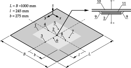
Figure 12. Geometry of a test square aluminium plate with damage arrangement: 1—measurement area, 2—PZT actuator, 3–7—additional masses, 8—notch cut, 9—epoxy glue, 10—aluminium plate, 11—electrical conductive adhesive and ± —electrodes.
Download figure:
Standard imageDuring measurements as the excitation signal a 35 kHz five-cycle sine pulse modulated by the Hann window was used. For each grid point measurements were repeated 20 times and the resulting signals were averaged to improve the signal-to-noise ratio. Between each measurement a time interval of 50 ms was kept in order to ensure fading out of previously generated elastic waves. The sampling frequency was set up to 512 kHz and 1024 time samples were registered during each measurement that covered 2 ms. Table 1 presents certain selected parameters of the PZT transducer used in experimental measurements [43].
It is typical for LSV measurements that, for a small number of points, a lower signal-to-noise ratio is achieved based on the fact that not enough reflected light returns back to a scanning head. All such points are characterized by much bigger RMS values. In order to reduce this effect median filtering in the space domain with 3 × 3 point window was applied. Examples of registered elastic wave propagation patterns in the aluminium plate under consideration are presented in the form of six arbitrary chosen time snapshots. Figure 13 illustrates the propagation of Lamb waves in the plate with one additional mass attached to its surface.
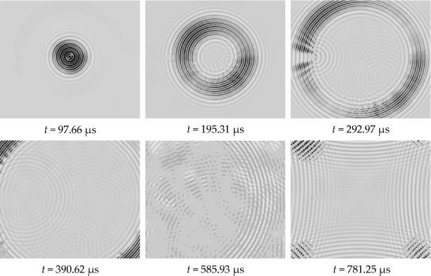
Figure 13. Evolution of wave propagation patterns in time for a square aluminium plate with single damage based on results of experimental measurements of the transverse displacement component by 1D LSV.
Download figure:
Standard imageTable 1. Selected parameters of PZT transducer used in experimental tests [43].
| Aluminium plate | Composite plate | |
|---|---|---|
| Type | T216-A4NO-373X | T216-A4NO-573X |
| Diameter (mm) | 31.8 | 63.5 |
| Rated voltage (Vp) | ±180 | ±180 |
| Resonant frequency (Hz) | 1170 | 290 |
| Free deflection (µm) | ±119 | ±476 |
Due to the fact that the introduced damage in the form of additional mass was a structural discontinuity, propagating elastic waves were reflected from the discontinuity and, as a consequence, damage became a source of new waves. This effect is clearly visible in figure 13 at time t = 292.97 µs and may be easily adopted for damage detection and localization purposes. However, in the case of multiple damage it can be difficult to detect and localize all defects, as is presented in figure 14. For more precise recognition of damage-related patterns the RMS function can be applied, as proposed theoretically in section 4.

Figure 14. Evolution of wave propagation patterns in time for a square aluminium plate with multiple damage based on results of experimental measurements of the transverse displacement component by 1D LSV.
Download figure:
Standard imageBecause elastic waves are reflected from various damage-related discontinuities the distribution of associated scattered energy within the plate is also changed. These subtle changes can also be associated with changes in the RMS values and therefore can be used for damage detection and localization purposes. However, relatively large values of the RMS function usually dominate in the areas near the excitation points and, as a result, almost the whole range of scale values is associated with this small area. In order to overcome that problem the authors propose to use a logarithmic scale for the values of the RMS function calculated. Figures 15 and 16 present RMS and logarithmic RMS damage maps for the square aluminium plate under investigation calculated based on all 1024 time samples, i.e. covering the total time span of 2 ms.

Figure 15. RMS and logarithmic RMS damage maps for a square aluminium plate with no damage, based on results of experimental measurements of the transverse displacement component by 1D LSV (t1 = 0 ms, wk = 1).
Download figure:
Standard image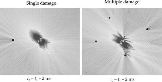
Figure 16. Logarithmic RMS damage maps for a square aluminium plate with single or multiple damage based on results of experimental measurements of the transverse displacement component by 1D LSV (t1 = 0 ms, wk = 1).
Download figure:
Standard imageFollowing the results of numerical simulations presented in section 4 it can be said that in the case of unweighted RMS damage maps (wk = 1) the patterns observed in RMS maps are strongly dominated by the excitation source. This has a masking effect on any damage-related features, especially those originating from damage distant from the excitation source.
In order to equalize and smooth the distribution of the RMS function in the whole area under investigation the subsequent time samples were multiplied by a weighting factor, as proposed in equation (13) in section 4. A comparison of such evaluated RMS damage maps for the first 256 time samples, i.e. covering the total time span of 0.5 ms, and for different values the weighting factors wk are presented in figures 17 and 18.
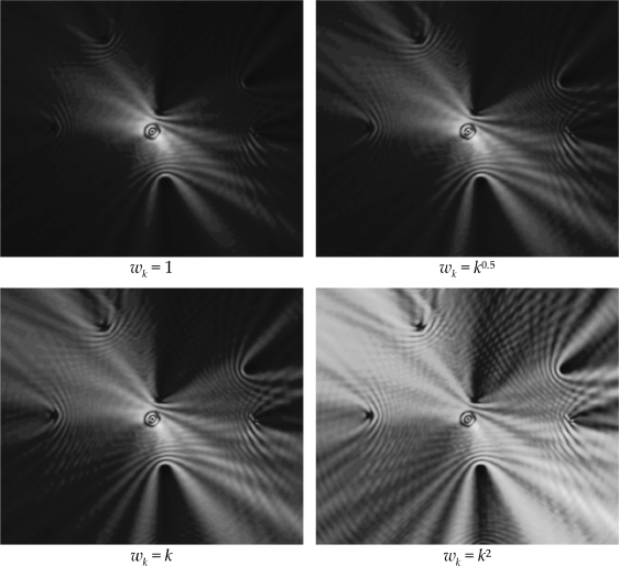
Figure 17. The influence of weighting factors wk on RMS damage maps for a square aluminium plate with multiple damage based on results of experimental measurements of the transverse displacement component by 1D LSV (t1 = 0 ms, t2 − t1 = 0.5 ms).
Download figure:
Standard image
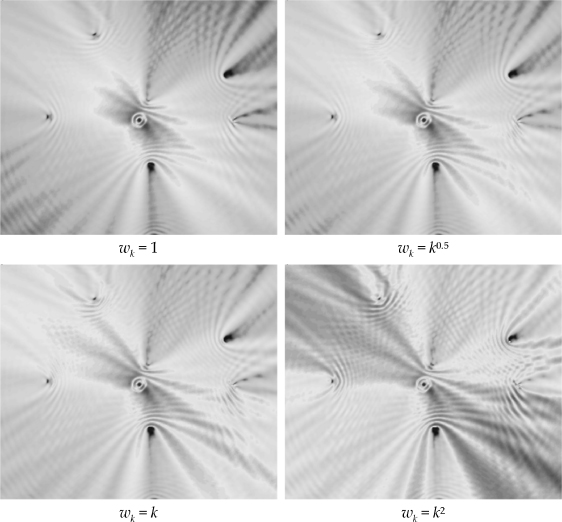
Figure 18. The influence of weighting factors wk on logarithmic RMS damage maps for a square aluminium plate with multiple damage based on results of experimental measurements of the transverse displacement component by 1D LSV (t1 = 0 ms, t2 − t1 = 0.5 ms).
Download figure:
Standard imageIn general it can be said that the resolution of RMS damage maps can be easily and effectively increased by the use of different values of the weighting factors wk, as presented earlier in section 4 in the case of the results of numerical simulations by the SFEM. The results obtained from experimental measurements by LSV confirm that better resolution corresponds to higher values of the weighting factor wk, i.e. for linear wk = k or square wk = k2 weighted RMS damage maps. However, attention must be paid in order to minimize the influence of the boundary reflected waves. This can be very well observed in the case of results presented in figure 17.
On the other hand, in the case of logarithmic RMS damage maps the influence of the weighting factors wk is much less prominent and relatively good resolution of the maps can be obtained, even of the unweighted case, i.e. when the weighting factor wk = 1, as clearly seen from figure 18. As shown earlier in section 4 an appropriately chosen sampling interval Δt has great influence on the resulting RMS damage maps. Figure 19 illustrates this influence on the sensitivity of weighted logarithmic RMS damage maps.

Figure 19. Evolution of logarithmic RMS damage maps in time for a square aluminium plate with multiple damage based on results of experimental measurements of the transverse displacement component by 1D LSV (t1 = 0 ms, wk = k2).
Download figure:
Standard image4.2. Composite plate
As the second object of experimental measurements a square, 3.2 mm thick, composite plate was investigated. The plate was composed out of four material layers, for which the reinforcement was glass fibres and the matrix was epoxy resin. The layers were arranged symmetrically as [0°/90°]s. The position of a PZT actuator with the location of the measurement area together with damage arrangement is presented in figure 20. A similar measurement area was used as for the square aluminium plate previously investigated, which consisted of 331 vertical lines and 281 horizontal lines, forming a rectangle of 600 mm × 500 mm and including 93 011 points. The intersection point of the rectangle's diagonals coincided with the plate centre and was the source of Lamb waves. In a similar manner as before, damage to the composite plate under investigation was simulated by four small additional masses: 1.6 g (3) and 3.2 g (4–6), fixed to the top surface of the plate.

Figure 20. Geometry of a test square composite plate with damage arrangement: 1—measurement area, 2—PZT actuator, 3–6—additional masses, 7—composite plate and ± —electrodes.
Download figure:
Standard imageDuring measurements as the excitation signal a 10 kHz four-cycle sine pulse modulated by the Hann window was used. As before for each grid point measurements were repeated 20 times and the resulting time signals were averaged to improve the signal-to-noise ratio. Between each measurement a time interval of 50 ms was kept in order to ensure fading out of previously generated elastic waves. The sampling frequency was set up to 256 kHz and 1024 time samples were registered during each measurement that covered 4 ms. Certain selected parameters of the PZT transducer used in experimental measurements [43] are presented in table 1.
The results of experimental measurements presented in figure 21 correspond to the case of the plate with multiple damage, where two additional masses 5 and 6 were attached to the plate surface. It can be clearly seen from the wave propagation patterns registered and shown in figure 21 that, due to plate material orthotropy, the elastic waves that propagate within the plate have different velocities in two perpendicular directions. Also damage-reflected waves are very well visible at time t = 585.94 and 781.25 µs. However, it should also be pointed out that a relatively small distance between masses 5 and 6, in comparison to the length of propagating waves, causes that their simultaneous detection and localization cannot be successfully performed based only on the wave propagation patterns registered by LSV.
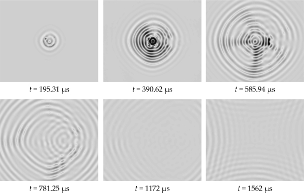
Figure 21. Evolution of wave propagation patterns in time for a square composite plate with multiple damage based on results of experimental measurements of the transverse displacement component by 1D LSV.
Download figure:
Standard imageFigure 22 presents logarithmic RMS damage maps obtained for two different damage scenarios. Only two additional masses at the same time were considered in each damage scenario, i.e. masses 3 and 4 (case 1) or masses 5 and 6 (case 2). In both these cases the logarithmic RMS damage maps were calculated based on the first 256 samples, i.e. covering the total time span of 1 ms. As can be clearly seen from figure 22 the use of the RMS or logarithmic RMS damage maps is very effective, enabling both detection and localization of the additional masses. It should be pointed out that the use of the RMS damage map revealed clearly the location of additional mass 6 hidden behind mass 5 (case 2) on a direct wave propagation path from the PZT transducer.
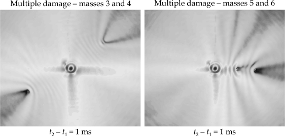
Figure 22. Logarithmic RMS damage maps for a square composite plate with multiple damage based on results of experimental measurements of the transverse displacement component by 1D LSV (t1 = 0 ms, wk = 1).
Download figure:
Standard image4.3. PZL W-3A helicopter stabilizer
The third object of experimental measurements was a composite stabilizer of a PZL W-3A helicopter, shown in figure 23. In this case the measurement area consisted of 475 vertical lines and 291 horizontal lines, which was approximately equal to a rectangle of 845 mm × 510 mm and included 138 225 grid points. As before, the intersection point of the rectangle's diagonals was the source of Lamb waves and the location of a PZT actuator. For that purpose a Sonox CeramTec PZT element of 10 mm diameter was used and the actuator was fixed to the stabilizer by PCB Petro Wax, as presented in figure 24.

Figure 23. Composite stabilizer of a PZL W-3A helicopter used for experimental measurements by 1D LSV.
Download figure:
Standard image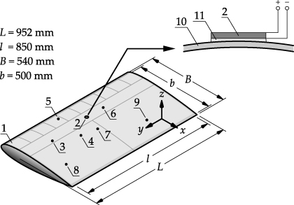
Figure 24. Geometry of a composite stabilizer of a PZL W-3A helicopter with damage arrangement: 1—measurement area, 2—PZT actuator, 3–9—additional masses, 10—composite stabilizer, 11—PCB Petro Wax and ± —electrodes.
Download figure:
Standard imageDuring measurements as the excitation signal a five-cycle sine pulses of various values of carrier frequencies fc modulated by the Hann window were used. Measurements for each point of the grid were repeated 20 times and the signals obtained in this way were averaged in order to improve the signal-to-noise ratio. Between each measurement of 1024 time samples a time interval of 20 ms was kept in order to ensure the fading out of previously generated elastic waves. The time span and the sampling frequency of the measurements was dependent on the carrier frequency fc of the excitation signal and were equal to: 4 ms and 256 kHz for the carrier frequency fc = 17.5 kHz, 2 ms and 512 kHz for the carrier frequency fc = 35 kHz, 0.8 ms and 1280 kHz for the carrier frequency fc = 100 kHz and 0.4 ms and 2.56 MHz for the carrier frequency fc = 250 kHz. Damage to the stabilizer was simulated by a number of small additional masses: 0.2 g (3, 4), 0.5 (5–7) and 1.6 g (8, 9), fixed to the top surface of the stabilizer, as presented in figure 24.
The results of experimental measurements presented in figure 25 were obtained for the lowest value of the carrier frequency fc = 17.5 kHz and were related to the case of the stabilizer with multiple damage, where all additional masses were attached to the upper surface of the stabilizer. However, contrary to the two cases of the aluminium and composite plates previously studied, the complex geometry of the stabilizer and its material properties resulted in wave propagation patterns carrying out very little visible information about any presence of damage. This was also observed for the remaining higher values of the carrier frequencies fc considered. Despite this fact, calculation of RMS or logarithmic RMS damage maps based on the signals registered by LSV revealed the presence of damage, but the maps obtained were strongly dependant on the values of the carrier frequency of propagating elastic waves fc, which, on the other hand, was very closely related to the damping properties of the composite material used for the stabilizer manufacturing and resulting energy distributions.
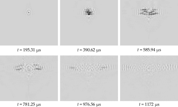
Figure 25. Evolution of wave propagation patterns in time for a composite stabilizer of a PZL W-3A helicopter with multiple damage based on results of experimental measurements of the transverse displacement component by 1D LSV.
Download figure:
Standard imageAs can be clearly seen from the logarithmic RMS damage maps presented in figure 26 simultaneous detection and localization of all additional masses could not be performed for one single carrier frequency fc due to different penetration ranges of propagating elastic waves within the structure of the stabilizer (i.e. different inspection areas). For the lowest value of the carrier frequency fc = 17.5 kHz the largest penetration range was obtained and, at the same time, additional masses 8 and 9 located relatively far from the excitation point could be successfully detected and localized as well as masses 3 and 6 located on the wave propagation path along the spur of the stabilizer. It is interesting to note that in this case the close range resolution was relatively low, and detection and localization of the remaining additional masses was difficult based on the RMS damage map obtained. When the value of the carrier frequency was increased to fc = 35 kHz the energy distribution associated with propagating elastic waves within the structure of the stabilizer was reduced to the area closer to the excitation point. This resulted in an improved resolution of the map obtained and, as a consequence, masses 4, 5 and 7 could be easily detected and localized, whereas detection and localization of masses 8 and 9 became difficult. Any further increase in the value of the carrier frequency fc resulted in a following decrease in the wave penetration range as well as in the signal-to-noise ratio. In the case of the carrier frequency fc = 100 kHz only masses 4 and 5 as the closest to the excitation point could be detected and localized together with masses 3 and 6 located on the spar. For the highest value of the carrier frequency fc = 250 kHz only mass 6 could be effectively detected and localized due to a very low signal-to-noise ratio.
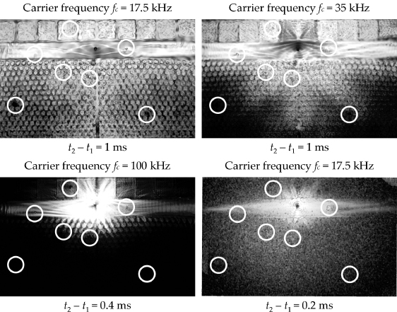
Figure 26. Logarithmic RMS damage maps for a composite stabilizer of a PZL W-3A helicopter with multiple damage based on results of experimental measurements of the transverse displacement component by 1D LSV—damage positions indicated by white circles (t1 = 0 ms, wk = 1).
Download figure:
Standard image4.4. Signal processing for short RMS measurements
All results presented in the three previous sections were obtained based on very precise experimental measurements. Unfortunately the assurance of this high precision required 14 h long tests. Such time-consuming measurements are, however, unacceptable from any practical point of view and should be significantly reduced in order to make this technique attractive for more realistic applications. Thus the authors examined an approach in which the long experimental testing was significantly shortened, preferably without any loss in the quality of the final result. This is demonstrated in the case of the square aluminium plate previously analysed. For experimental measurements the total number of grid points was reduced from an initial 93 011 to 9000 and any signal averaging was skipped. In this way the time required for the measurements was reduced nearly 200 times to 5 min only. In order to verify the quality of the signals registered by LSV and their further applicability for damage detection purposes and generation of RMS damage maps linear and cubic spline interpolations in the space domain were tested. The results obtained are presented in figure 27.

Figure 27. The influence of signal processing on logarithmic RMS damage maps for a square aluminium plate with multiple damage based on results of experimental measurements of the transverse displacement component by 1D LSV (t1 = 0 ms, t2 − t1 = 0.5 ms).
Download figure:
Standard imageAs can be seen from figure 27 linear interpolation in the space domain of the RMS damage map based on the raw signal had no significant improvement in the resulting RMS damage map. The obtained patterns in both raw and interpolated RMS damage maps are practically identical. A certain improvement in comparison with the linearly space-interpolated RMS damage map is obtained when cubic spline interpolation in the space domain is used. However, the best results were obtained in the case when the interpolation process was firstly performed on each time frame registered rather than on the resulting RMS damage map itself, which again was equivalent to cubic spline interpolation in the space domain. It should be emphasized that the resulting RMS damage map interpolated in this manner had practically the same resolution and quality as the original RMS damage map shown in figure 18 in section 4.
5. Conclusions
Based on the results of numerical and experimental measurement it can be concluded that damage maps based on the application of integral indices can be successfully employed for damage detection and localization in various structural elements. Out of two such indices assessed by the authors the RMS (root mean square) index is more sensitive to damage than the IMV (integral mean value) index and at the same time is much less sensitive to environmental noise. In the case of the composite materials, where propagating guided waves are strongly attenuated, results obtained by the use of the RMS index can be improved by appropriate signal weighting process. The weighting process also offers improved detection and localization of damage distant from the excitation point as well as located close to structural boundaries. Also logarithmic values of RMS functions allows easier damage recognition.
In practical applications RMS damage maps based on experimental measurements by LSV (laser scanning vibrometry) can be produced in a relatively short time, i.e. reaching 4 min for the area of 500 mm × 500 mm, all thanks to the use of relatively sparse grids of measurement points together with appropriate signal processing techniques. According to the results presented by the authors the best results were observed when spline interpolation in the space domain for all time samples was applied.
Acknowledgments
The authors of this work would like to gratefully acknowledge the support for this research provided by the Polish Ministry of Science and Higher Education through the European Funds System under the Sectoral Operational Programme Improvement of the Competitiveness of Enterprises via the MONIT project (Monitoring of Technical State of Construction and Evaluation of Its Lifespan) no. POIG.01.01.02-00-013/08.