
Abstract
This paper presents an investigation on the numerical simulation of Lamb wave propagation problems in plate-like structures. Based on the simple plate theory with six variables and extended Chebyshev nodes, a novel formulation of two-dimensional spectral finite elements (2D SFEs) with and without a lead zirconate titanate (PZT) layer is proposed. A simple technique is used in the formulations to avoid inherent thickness locking, which exists in the simple plate theory. Contrary to the existing methods, only one voltage degree of freedom is introduced for each PZT element. Formulations have been worked out in detail, and analysis of the base plates with and without PZTs has been carried out. The accuracy of the proposed 2D SFE is verified by comparing the simulations to data obtained by the finite element method-base commercial software ANSYS with very fine meshes and with existing experimental data. Numerical results indicate that the proposed method is efficient in simulating Lamb wave propagation in plate-like structures.
Export citation and abstract BibTeX RIS
1. Introduction
Lamb waves, with the advantages of small attenuation in long-distance propagation and high sensitivity to minute damage, have been widely used in structural health monitoring (SHM) for decades. For the purpose of designing an aircraft SHM network based on Lamb waves, it is necessary to have a fundamental understanding of the Lamb wave propagation properties in plate-like structures. This requires a reliable physics model and an efficient numerical approach.
The conventional finite element method (FEM) [1, 2], as one of the most efficient numerical methods, is often used to obtain numerical simulations of wave propagation in structures. The diagnosed Lamb waves induced and received by PZT transducers have less than a few tenths of a millimeter as a minimum wavelength. To accurately catch the wave scattering by boundaries, the potential damage and the surface-bonded transducers in structures, high discretization of the model is required. Thus, models of complex structures based on conventional FEM inevitably lead to impractical computational time and memory.
Compared with FEM, the spectral finite element method (SFEM) exhibits an exponential convergence rate. As a more promising tool to investigate the characteristics of Lamb wave propagation in plate-like structures, the SFEM has been studied by many researchers [3–12]. In general, the SFEM for plate-like structures can be classified into two categories: (1) three-dimensional (3D) SFEM [6–8], which usually has a large number of element nodes or a great number of degrees of freedom (DOFs). Although the high computational accuracy is retained, the computational efficiency is reduced; (2) two-dimensional (2D) SFEM [3, 4, 9, 10], developed based on plate theories such as the first-order shear deformation theory (FSDT), higher-order plate theories (HOPT) or their variants. The simulation of Lamb wave propagation in plate-like structures by the 2D SFEM is obviously more efficient than by the 3D SFEM, since the 2D element has fewer nodes and DOFs but can meet the solution accuracy by pre-integration of the element mass/stiffness matrix across the thickness. The PZT transducers with circular shapes are modeled by using either isoparametric elements [6] or subparametric elements or by using a semi-analytical method [11, 12].
For accurate simulations of the Lamb wave propagation in plates, one should pay attention to a locking phenomenon, called thickness locking or Poisson locking and occurring for nonzero Poisson's ratios [13–15], since the thickness locking may degrade the numerical solution accuracy. One way to overcome this defect is by adopting quadratic, cubic or higher-order displacement distribution through the thickness, introducing more nodes or variables across the thickness. Willberg et al [16] suggested that a quadratic polynomial through the thickness is needed when higher-order finite element schemes are to be used for simulating Lamb wave propagation in plates. Chang and his coworkers [6] solved PZT-induced Lamb wave propagation problems by adopting 3D SFE with six nodes in the thickness direction. The simulations agree well with the experimental results since the thickness locking disappears. It is obvious, however, that the 3D solid SFEM is not efficient for simulating the Lamb wave propagation in plates. To improve the computational efficiency, Chang and his coworkers [17] proposed a hybrid spectral element with only two nodes in the thickness direction. They achieved the goal of computational efficiency to a certain extent, but the computational accuracy may be lost since the thickness locking may occur with the usage of linear interpolation functions in the thickness direction.
For the development of 2D SFEs, some assumptions are introduced in the plate theories to simplify the 3D plate-like structures. Carrera and Brischetto [15] pointed out that due to coupling between the transverse normal strain and the in-plane strains in the constitutive law, thickness locking occurs when simplified kinematic assumptions are introduced in the plate theories. More precisely, thickness locking will appear if the distribution of transverse normal strain  is assumed constant through the thickness [18].
To the best of the authors' knowledge, it seems that thickness locking in 2D SFEs for simulating Lamb wave propagation in plates has not been well addressed in the literature thus far. Therefore, the aim of the paper is to fill that gap. Based on the first-order shear deformation theory with only a linear variation in the thickness direction, a new efficient and accurate 2D SFE is proposed. A simple way [19] is used to avoid the inherent thickness locking in the formulation of the element stiffness matrix. To validate the proposed element, numerical results obtained by the proposed element are compared with those obtained by ANSYS with very fine meshes and existing experimental data. The effect of thickness locking on the simulations is demonstrated. Some conclusions are drawn based on the results reported herein.
2. Formulation of a 2D spectral finite element
2.1. Displacement and strain fields
Consider a PZT-bonded base plate that refers to the global coordinate system (x, y, z) located on the mid-plane of the base plate, as shown in figure 1. If the excitation frequency is not too high, the first-order shear deformation theory (FSDT), which takes the effect of the lateral contraction in the z-direction into account [4, 20], can be adopted in modeling Lamb wave propagation in plate-like structures. Theoretical analysis demonstrates that the simple plate theory can be used when the product of the wave frequency and the plate thickness is within 1.0 MHz mm, although the Lamb wave structure can be fairly complicated. Details on this issue can be found in the appendix.

Figure 1. Kinematic parameters used for the description of a PZT-bonded base plate.
Download figure:
Standard image High-resolution imageAccording to the first-order shear deformation theory, the displacement fields for the base plate are given by
where the subscripts A and S represent the anti-symmetric and symmetric modes,  ,
,  and
and  are the in-plane and out-of-plane displacements on the mid-plane of the base plate,
  and
and  are the rotations of the cross section normal to the mid-plane of the base plate,
  is the lateral contraction and t is time, respectively. Note that
  ,
,  and
and  are related to the symmetric modes, and
  ,
,  and
and  are related to the anti-symmetric modes.
To employ the simple way shown in [19] to avoid the inherent thickness locking in the simple plate theory, the strain fields of the base plate are also decomposed into anti-symmetric and symmetric modes, namely
For the PZT layer, the displacement fields are given by
where  ,
,  and
and  are the in-plane and out-of-plane displacements on the mid-plane of the PZT layer,
  and
and  are the rotations of the cross section normal to the mid-plane of the PZT layer,
  is the lateral contraction and
  is the distance between the mid-planes of the base plate and the PZT layer, shown in figure 1.
Since the PZT layer is perfectly bonded on the base plate, the displacements at the interface should be compatible. After some manipulations, one has
where

and the strains in the PZT layer can be given by
An assumption is made that the electric potential for the PZT layer is distributed linearly through the thickness [21, 22]. The electric voltage is equal to zero on the lower surface of the PZT layer and is equal to V on the upper surface of the PZT layer. Therefore, the electric voltage  in the PZT layer can be calculated by

The resulting electric field  is
is

where  is the thickness of the PZT layer, and
 ![$[{{{\bf B}}_{V}}]=[1/{{h}_{p}}]$](https://content.cld.iop.org/journals/0964-1726/23/9/095018/revision1/sms498054ieqn24.gif) .
.
2.2. Constitutive equations
Equation (2) expresses three-dimensional (3D) strain fields; however, the 3D constitutive equations should not be used directly. Otherwise, thickness locking would occur if no remedial measure was used since the displacement shown in equation (1) varies only linearly through the plate thickness.
It is known that anti-symmetric modes are primarily flexural waves and are more likely to be influenced by thickness locking [16]. Equation (2) shows that  . However,
  due to Poisson's effect. In other words,
  for nonzero
  or
or  . This contradiction, known as thickness locking, can be avoided if a plane stress state is assumed [19]. In this way,
  is not involved in equation (9) to calculate the stress components. Alternatively, it is observed that the anti-symmetric displacement components, shown in equation (1), are exactly the same as the ones in the well-known Mindlin plate theory. Therefore, the plane stress state as adopted in the Mindlin plate theory should also be employed for the anti-symmetric mode.
In summary, the 3D constitutive equation is only used for the symmetric strains, and a different constitutive equation is used for the anti-symmetric strains [19]. In detail, the stress-strain equations are given by

where  and
and  are the 3D stress and strain vectors, the superscripts A and S represent the anti-symmetric and symmetric modes,
 ![$[{\bf C}]$](https://content.cld.iop.org/journals/0964-1726/23/9/095018/revision1/sms498054ieqn33.gif) and
and ![$[\tilde{{\bf C}}]$](https://content.cld.iop.org/journals/0964-1726/23/9/095018/revision1/sms498054ieqn34.gif) are given by
are given by
and
where
and
Equation (11) is obtained based on the assumption of the plane stress state and  is the shear correction factor as adopted in the Mindlin plate theory. In equations (12) and (13), E and v are the elasticity modulus and Poisson's ratio, respectively.
hp is much smaller than hb . However, hp /Lp is much larger than hb /Lb , where Lp and Lb are the smaller in-plane dimension of the PZT layer and the base plate. Besides, the PZT layer is usually bonded on the upper surface of the base plate; thus, pure anti-symmetric modes will not exist practically. Therefore, for the PZT layer, the 3D constitutive equations are used, namely

where ![$[{\bf e}]$](https://content.cld.iop.org/journals/0964-1726/23/9/095018/revision1/sms498054ieqn36.gif) and
and ![$[{{{\boldsymbol{ \varepsilon }} }^{S}}]$](https://content.cld.iop.org/journals/0964-1726/23/9/095018/revision1/sms498054ieqn37.gif) are matrices of the piezoelectric constant and the dielectric constant measured at zero strain and {D} and {E} are vectors of the electric displacement and electric field, respectively.
are matrices of the piezoelectric constant and the dielectric constant measured at zero strain and {D} and {E} are vectors of the electric displacement and electric field, respectively.
2.3. Mass and stiffness matrices
In developing a 2D spectral finite element without PZT layers, each node of the element owns six displacement degrees of freedom  , i.e.,
  and
and  . Thus, the total number of DOFs is the same as the hybrid spectral element in [17] if the node distribution in the
  plane is the same. For a 2D SFE with one PZT layer, each node of the element owns nine displacement degrees of freedom
  , i.e.,
  and
and  .
.
In the proposed 2D spectral finite element with a PZT layer, each PZT element shares only one conjunct voltage DOF V, no matter how many SFEs are used to model the PZT element. In other words, each PZT element (actuator or sensor) has only one voltage DOF. This is quite different from the existing methods [2, 6, 8] in that each node has one voltage DOF, and the weighted average of all of the voltage DOFs is taken as the voltage applied on the PZT element. It is obvious that the proposed approach is beneficial to the CPU time in numerical simulations, especially when the PZTs are modeled by more than one spectral finite element, or the total number of voltage DOFs is large.
It is known that if the extended Chebyshev points are used as the element nodes, a larger time step can be used in the numerical integration by the central difference method [23]. The non-dimensional node position in [−1, 1] can be explicitly computed by
For illustration, a 6 × 6 node 2D SFE, shown in figure 2, is presented. The element contains a PZT layer, and each node has nine DOFs.

Figure 2. Nodal distribution of a 6 × 6-node 2D spectral finite element.
Download figure:
Standard image High-resolution imageThe nine displacements within the element can be expressed as
where ![$[{\bf N}]$](https://content.cld.iop.org/journals/0964-1726/23/9/095018/revision1/sms498054ieqn45.gif) is the shape function matrix,
is the shape function matrix,  are shape functions,
  and
and  are Lagrange interpolation functions and {q} is the vector of the nodal DOFs, respectively.
Element strain fields can be obtained by substituting equation (16) into equations (2) and (6). One has
Based on the virtual work principle or on Hamilton's principle [2, 6], a set of equations of motion for each element can be derived and written in a matrix form as
where
 is the determinant of the Jacobian matrix, and
  and
and  are the mechanical force vector due to the applied load and the applied electrical charge on the surface of the PZT layer, respectively.
Note that [BV
] is given by equation (8), each PZT element (actuator or sensor) has only one voltage DOF and ![$\int {{\Omega }_{b}} {{[{\bf B}_{b}^{A}]}^{T}}[{\bf C}][{\bf B}_{b}^{S}]d\Omega =\int {{\Omega }_{b}} {{[{\bf B}_{b}^{S}]}^{T}}[\tilde{{\bf C}}][{\bf B}_{b}^{A}]d\Omega =0$](https://content.cld.iop.org/journals/0964-1726/23/9/095018/revision1/sms498054ieqn52.gif) , where
, where  is the domain of integration defined in the base plate. The Gauss quadrature is used for obtaining the element matrices in equation (19). The diagonal mass matrix can be obtained by the method of row summation before performing the numerical integration [23].
For the base plate model without PZTs, simply remove the terms associated with the PZT layer. Thus, one has

The well-known explicit time-integration scheme, called the central difference method, is adopted to solve equation (18) or equation (20).
To model irregular shapes, the method of the sub-parametric element is adopted. The order of geometric functions is relatively lower than the order of displacement functions. The geometric functions are defined by
where x and y are the space variables defined on the physical domain of the element, and  are the variables defined on the bi-unit square domain, shown in figure 2.
  are coordinates of nodes on the element boundaries and M is the total number of boundary nodes; thus,
  are the shape functions for serendipity type finite elements with only boundary nodes.
The first order derivatives of shape functions  with respect to the space variables x and y can be computed by

With equation (21) and the given  , the Jacobian matrix can be computed by

3. Numerical analysis and discussions
3.1. Model definition
In order to verify the validity of the proposed 2D SFE established by the simple plate theory, two models with free boundary conditions are considered: (1) a base plate without PZTs and (2) a PZT bonded on the top of the base plate. For the convenience of analysis, assume that the two models shown in figure 3 are in the state of plane strain, similar to the models employed in [6, 16]. To be more specific, both models have a sufficiently large dimension in the y direction.
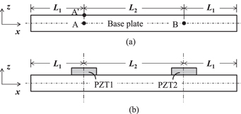
Figure 3. Geometry of two-dimensional models: (a) model of the base plate without PZTs, (b) model of the base plate with bonded PZTs.
Download figure:
Standard image High-resolution imageIn figure 3(a), points A and B are on the mid-plane of the base plate, a force is actuated at point A' and the displacement signal is the output at point B. In figure 3(b), a pitch-catch method using a pair of piezoelectric actuators (PZT1) and sensors (PZT2) is introduced.
The base plate has a total length of L = 2L1 + L2 and has the thickness of hb . The base plate material is aluminum, and the material properties are E = 70.0 GPa, ν = 0.3 and ρb = 2700 kg m−3. The material properties of PZTs are listed in table 1.
Table 1. Material properties of PZTs.
| Properties | Value | Properties | Value |
|---|---|---|---|

|
147.0 GPa |

|
−3.09 C m−2 |

|
105.0 GPa |

|
16.0 C m−2 |

|
93.7 GPa |

|
11.6 C m−2 |

|
113.0 GPa |

|
1130 |

|
23.0 GPa |

|
914 |

|
21.2 GPa |

|
7700.0 kg m−3 |
In numerical simulations, a frequency of the force or the voltage input signal is chosen to guarantee that only the lowest symmetric S0 mode and the lowest anti-symmetric A0 mode are excited. In the present investigation, hb = 1.02 mm and hp = 0.25 mm; therefore, both input signals have a center frequency of 100 kHz and a time duration of 50 μs, as shown in figure 4.
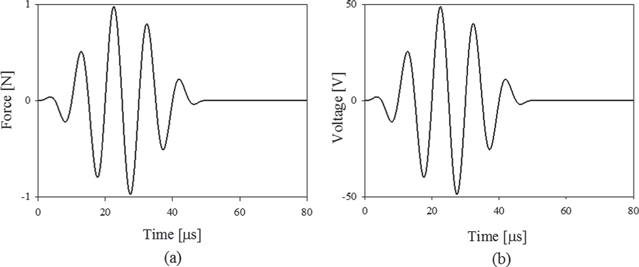
Figure 4. Excitation signals: (a) a force input signal, (b) a voltage input signal.
Download figure:
Standard image High-resolution imageDuring numerical simulations, it is possible that both the A0 and S0 modes are received simultaneously at point B or by sensor PZT2 since the speeds of the A0 and S0 modes are quite different, and the reflected S0 wave from the edge of the base plate may propagate to point B or sensor PZT2 when the slower A0 wave reaches there. This makes it difficult to recognize or distinguish different Lamb wave modes and makes the calculated velocities inaccurate, or it can even cause them to make no sense. Hence, in order to completely separate the two Lamb wave modes during the simulations, the distance between point A and point B or between PZT1 and PZT2 should be carefully selected.
For illustration, take the base plate model without PZTs as an example. Three propagation paths are considered, namely path #1: S0 mode propagates from point A directly to point B; path #2: A0 mode propagates from point A directly to point B; and path #3: S0 mode propagates from point A to the left end of the base plate, and then the reflected S0 mode propagates to point B. To distinguish the three Lamb wave modes from the signal picked up at point B, the waves propagating along these three paths should reach point B at different times or satisfy the following relations:

where the subscripts p1 – p3 represent path #1 – path #3, respectively.
Taking the wave packet width of the S0 and A0 modes into consideration and assuming that they have the same width as the input signal, equation (24) should be modified by
where  represent the analytical group velocities of the S0 and A0 modes, and
  is the wave packet width of the input signal.
In the present investigation, the geometric dimensions are chosen according to equation (25). They are L1 = 406.4 mm and L2 = 177.8 mm and are different from the ones used in [6]. If the dimensions in [6] are used, then the speed of the A0 mode cannot be accurately calculated by the so-called A0 signal that was picked up by PZT2 since it actually contains both A0 and reflected S0 waves.
3.2. The model of the base plate without PZTs
Consider first the model of the base plate without PZTs. The plate is modeled by 312 proposed SFEs. For verification, the same model is also analyzed by using ANSYS. In ANSYS, four rectangular plane strain elements (2D plane182) are used in the thickness direction; thus, the finite element model has a total of 14 976 elements. Figure 5 shows the applied load format used in ANSYS and in the SFEM. In ANSYS, a force Fx , shown in figure 5(a), is applied at point A' on the upper surface of the plate. The same force Fx and the resulting bending moment My = Fx hb/2 are applied at point A' in the SFEM, shown in figure 5(b). The Fx applied at point A excites the S0 mode, and My excites the A0 mode. For simplicity and for convenience in discussions, symbols SFEσz and SFE3D stand for the proposed 2D SFE and for the one based on the 3D constitutive equations, without taking any remedial measure for the thickness locking, respectively.

Figure 5. Load configurations: (a) in ANSYS, (b) in the SFEM.
Download figure:
Standard image High-resolution imageMore precisely, the only difference between SFE3D and SFEσz is the way in which to compute the stress components. SFEσz directly uses equation (9) to compute the stress components. SFE3D also uses equation (9) to compute the stress components but with some modifications, i.e., replacing matrix ![$[\tilde{{\bf C}}]$](https://content.cld.iop.org/journals/0964-1726/23/9/095018/revision1/sms498054ieqn73.gif) in equation (9) by matrix [C]. All of the other mathematic formulations for the two approaches are exactly the same.
in equation (9) by matrix [C]. All of the other mathematic formulations for the two approaches are exactly the same.
Figures 6(a) and (b) compare the components of displacement  and
and  at point B obtained by SFEσz with those obtained by ANSYS. From equation (1), it is known that the
  and
and  at point B (z = 0) are the S0 and A0 modes. The S0 wave, excited by force Fx
, propagates along the right and left directions of point A simultaneously. The S0 wave propagating along the right direction reaches point B, which is the first wave package shown in figure 6(a). The S0 waves propagating along the left and right directions are reflected successively when they reach the left and right ends of the plate. The two reflected waves meet at point B at the same time, which is the second wave package, shown in figure 6. This explains why the amplitude of the second wave package is twice as high as that of the first wave package, shown in figure 6(a). The good agreement between the results obtained by SFEσz and those obtained by ANSYS demonstrates that the proposed 2D SFE is capable of simulating the propagation of Lamb waves in plates. It is also seen that the A0 mode with a relatively slower group/phase velocity exhibits more dispersive characteristics compared to the S0 mode.
at point B (z = 0) are the S0 and A0 modes. The S0 wave, excited by force Fx
, propagates along the right and left directions of point A simultaneously. The S0 wave propagating along the right direction reaches point B, which is the first wave package shown in figure 6(a). The S0 waves propagating along the left and right directions are reflected successively when they reach the left and right ends of the plate. The two reflected waves meet at point B at the same time, which is the second wave package, shown in figure 6. This explains why the amplitude of the second wave package is twice as high as that of the first wave package, shown in figure 6(a). The good agreement between the results obtained by SFEσz and those obtained by ANSYS demonstrates that the proposed 2D SFE is capable of simulating the propagation of Lamb waves in plates. It is also seen that the A0 mode with a relatively slower group/phase velocity exhibits more dispersive characteristics compared to the S0 mode.
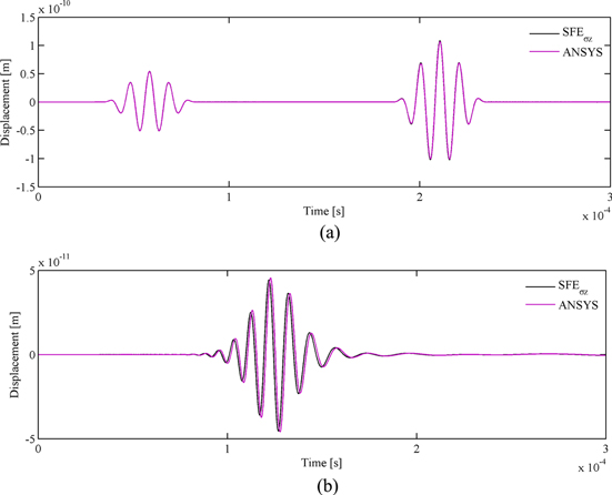
Figure 6. The displacement outputs: (a)  and (b)
  at point B using the modification of constitutive equations.
Download figure:
Standard image High-resolution imageIn the simulation, the time step is chosen as 3.0 × 10⁻⁸ s for the SFEM and 7.5 × 10⁻⁸ s for ANSYS. Table 2 shows the comparison of the computational resources. It is seen that the SFEM can get similar accurate results with a fewer number of DOFs and much less CPU time; thus, the computational efficiency is greatly increased.
Table 2. Comparison of computational resources.
| SFEM | ANSYS | |
|---|---|---|
| Total number of DOF | 6244 | 37 450 |
| CPU time | 43 s | 2340 s |
The results obtained by using the SFE3D are shown in figure 7. It is seen that the predictions of the S0 mode, shown in figure 7(a), agree well with the ANSYS data. However, a significant difference exists between the predictions of the A0 mode shown in figure 7(b) and the ANSYS data. From figures 6 and 7, one may conclude that thickness locking only exists in the anti-symmetric modes, and remedial measures are necessary to avoid the thickness locking.
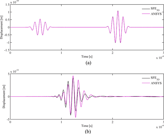
Figure 7. The displacement outputs: (a)  and (b)
  at point B directly using the 3D constitutive equations.
Download figure:
Standard image High-resolution imageTable 3 summarizes the group velocity that was obtained by numerical simulations and compared with theoretical solutions. To extract the accurate wave packet time of flight (TOF) from the signal, a time–frequency technique called the wavelet transform (WT) is used. Since the propagation distance is exactly known, the group velocity can be easily obtained. From table 3, it is seen that SFEσz shows extremely high accuracy for the case studied and is even higher than the data obtained by ANSYS with fine meshes. It is seen that the results of SFE3D are not satisfactory for the A0 mode. Due to thickness locking, the error reaches 4.54% for this simple case. The error will be increased with the increase of the center frequency [19]. This implies that remedial measures should be taken to avoid thickness locking, which exists inherently in the simple plate theory.
Table 3. Comparison of the group velocities of the A0 mode and S0 mode.
| A0 mode | S0 mode | |
|---|---|---|
| SFEσz | 1790.5 m s−1 (−0.084%) | 5336.8 m s−1 (0.034%) |
| SFE3D | 1873.5 m s−1 (4.54%) | 5336.8 m s−1 (0.034%) |
| ANSYS | 1780.1 m s−1 (−0.66%) | 5333.3 m s−1 (−0.032%) |
| Theoretical value | 1792.0 m s−1 | 5335.0 m s−1 |
3.3. The model of the base plate with PZTs
In practice, the input signal is usually induced by PZT actuators, and the output signals are picked up by PZT sensors. In this section, a model of the base plate with two surface-mounted PZTs, shown in figure 3(b), is investigated. The input voltage signal with an amplitude of 50 V is applied on the top surface of PZT1. The output voltage signal is measured by PZT2. The plate is modeled by 312 proposed SFEs, including four SFEs with PZTs. For verification, the same model is also analyzed using ANSYS. In Contrast to the previous case, besides 14 976 rectangular plane strain elements (2D plane 182), 24 additional rectangular plane strain elements (2D plane13) for each PZT transducer are used to model the two PZT elements. The mesh configurations for the 2D SFEM and the ANSYS models are schematically shown in figure 8.

Figure 8. Finite element mesh configurations for (a) 2D SFEM, (b) ANSYS.
Download figure:
Standard image High-resolution imageTo verify the usage of one voltage degree for each PZT element, the problem is analyzed by using the 2D SFE with different numbers of voltage degrees: one with only one voltage degree for the entire PZT element, the other with one voltage degree at each node. Although the magnitude of voltage at each node is quite different, the weighted sum of the voltage on the PZT element is the same as the one obtained by the 2D SFE with only one voltage degree for the entire PZT element. Due to space limitations, the detailed comparisons are omitted, and only the results obtained by the proposed SFEs are presented.
The simulation results, together with the data obtained by ANSYS, are shown in figure 9. The first and third waves are the S0 mode, and the middle one is the A0 mode. A similar phenomenon to the displacements shown in figures 6 and 7 is observed. The data obtained by the proposed SFEs, shown in figure 9(a), agree well with the ones by ANSYS with very fine meshes; thus, the proposed SFEs with and without PZTs are verified. Due to the thickness locking, however, the results obtained by the SFE3D, shown in figure 9(b), do not agree well with the ANSYS data for the anti-symmetric mode. It is demonstrated again that remedial measures should be taken to avoid thickness locking in formulating a 2D spectral plate element based on the simple plate theory.
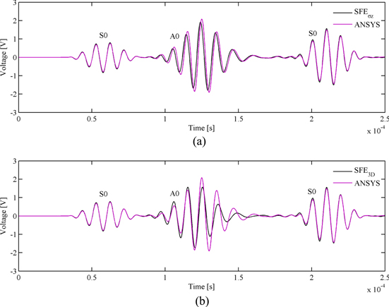
Figure 9. Sensor signals at PZT2 compared to ANSYS with (a) SFEσz and (b) SFE3D.
Download figure:
Standard image High-resolution imageTable 4 compares the group velocities of the A0 and S0 modes with three different methods. Again, the accuracy of the proposed SFE is the highest. Due to the presence of PZT elements, the error appears slightly larger than the base plate without PZTs, shown in table 3. It is reported in [20] that the PZT layer tends to decrease the group velocities of all the wave modes. Due to thickness locking, the error of the group velocity of the A0 mode predicted by SFE3D is much larger than the other two.
Table 4. Comparisons of the group velocity of the A0 mode and S0 mode.
| A0 mode | S0 mode | |
|---|---|---|
| SFEσz | 1785.1 m s−1 (−0.39%) | 5319.4 m s−1 (−0.29%) |
| SFE3D | 1869.6 m s−1 (4.33%) | 5322.8 m s−1 (−0.23%) |
| ANSYS | 1778.9 m s−1 (−0.73%) | 5315.0 m s−1 (−0.38%) |
| Theoretical value | 1792.0 m s−1 | 5335.0 m s−1 |
During the Lamb wave propagation, voltages will also be induced by the actuator PZT1, even after the input signal has finished. Figure 10 shows the output signal picked up by PZT1. With the group velocity of the S0 mode, listed in table 4, it is easy to distinguish the four Lamb wave modes. The first wave package with the largest voltage amplitude is excited by the input voltage signal, and the other three wave packages with much smaller amplitudes are all S0 modes, generated by the reflected Lamb waves coming from PZT2 and the left and right edges of the base plate, respectively.
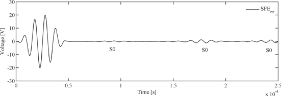
Figure 10. Voltage induced by PZT1.
Download figure:
Standard image High-resolution image3.4. 3D modeling of piezo-elastic dynamics for circular PZTs
To demonstrate the capability of the proposed 2D SFE for 3D modeling of piezo-elasto dynamics for PZTs with circular shapes, a pitch-catch model in [17] is analyzed by using the SFEσz. A 355.6 mm × 508.0 mm × 1.0 mm thick aluminum plate is instrumented with a pair of 6.35 mm radius, 0.25 mm thick PZTs on the upper surface of the plate, as shown in figure 11. PZT1 acts as an actuator, while PZT2 as a sensor. The entire plate is modeled by 17 920 proposed 2D SFEs, including eight SFEs with PZTs. For comparisons, the excitation signal and the material properties of the base plate and the PZTs are the same as the ones listed in [17].
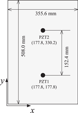
Figure 11. A pitch–catch model.
Download figure:
Standard image High-resolution imageSnapshots of the y-displacement of the induced waves on the top surface of the plate at four different time instances are shown in figure 12. The excitation frequency is 100 kHz. It can be clearly seen that only the S0 mode and the A0 mode are excited. The S0 mode has a large wavelength and a fast velocity, while the A0 mode has a small wavelength and a low velocity. When the Lamb waves encounter the free boundaries of the plate, they are reflected back into the plate.
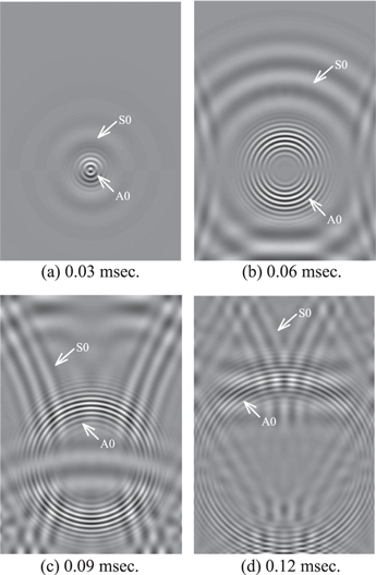
Figure 12. Snapshots of the y-displacement on the top surface of the plate.
Download figure:
Standard image High-resolution imageFigure 13 presents the comparison of the voltage results at PZT2 simulated by the proposed 2D SFEs to the experimental data directly cited from [17]. The excitation frequency is 100 kHz. It is seen that the simulated results correlate well with the experimental data in terms of the waveform. A similar correlation between the experimental data and the hybrid spectral element [17] is observed. Since one hybrid spectral element was used in the thickness direction, the total number of DOFs is the same as in the present model, if the same number of elements is used.
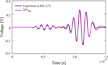
Figure 13. Voltage signal at PZT2 compared to the experimental sensor signal at 100 kHz.
Download figure:
Standard image High-resolution imageWhen the excitation frequency increases to 400 kHz, the simulated results by the proposed 2D SFEs are shown in figure 14. The agreement with the experimental data is not as good as the agreement shown in figure 13. Disagreements on the shape of the wave package, especially for the S0 mode, are clearly seen. A similar mismatch to the experimental data also exists for the results obtained by the hybrid spectral element in [17]. It is pointed out by Ha and Chang [17] that the mismatch is attributable to the interface adhesive layer since the effects of the adhesive layer are not considered in the simulations. In contrast to the case of 100 kHz, two hybrid spectral elements were used in the thickness direction to obtain reasonably accurate results. Since the present model uses one element in the thickness direction, the total number of DOFs is much smaller than the hybrid spectral element model in [17] for the case considered.

Figure 14. Voltage signal at PZT2 compared to the experimental sensor signal at 400 kHz.
Download figure:
Standard image High-resolution image4. Conclusions
In this paper, novel 2D spectral finite elements (2D SFEs) with and without a PZT layer are developed to simulate PZT-induced Lamb wave propagation in thin plates. In contrast to the existing method, the extended Chebyshev points are used as the element nodes, and only one voltage degree of freedom is introduced for each PZT element. The effect of thickness locking on the solutions is discussed, and a simple way to resolve this problem is demonstrated. An analysis of the base plate model with and without PZTs has been carried out. The accuracy of the proposed 2D SFE is verified by comparing the simulations to the results obtained by ANSYS with very fine meshes or with existing experimental data.
Based on the results reported herein, one may conclude that the accuracy of the proposed 2D SFE is high, although the simple plate theory is adopted in the formulations. It is seen that only the anti-symmetric modes suffer from the influence of thickness locking, and the introduction of the plane stress condition on the anti-symmetric mode can solve the problem effectively.
Acknowledgements
The work is partially supported by the National Natural Science Foundation of China (50830201) and by the Priority Academic Program Development of Jiangsu Higher Education Institutions.
Appendix.: Application range of linear across-the-thickness displacement assumption
Since the Lamb wave modes can be fairly complicated, the argument may arise that a linear representation may not be a good assumption, especially for higher order modes. To better understand the behavior of Lamb wave motion, a plane-strain PZT-structure shear layer coupling model [24, 25], shown in figure A.1, is used. An adhesive layer is considered, and the assumption is made that the adhesive layer acts only as a shear layer in which the mechanical effects are transmitted through the shear effects.
The PZT length is 2a, the base plate thickness is 2d and the material property is μ. Ideal bonding is assumed; thus, the adhesive layer is viewed as a pin force model, and all of the load's transfer occurs over an infinitesimal area of the PZT's ends. Using the space-domain Fourier analysis and the residue theorem, the Lamb wave displacements in the base plate are given by
where u(x, z, t) and w(x, z, t) are the in-plane and the out-of-plane displacements, τ0 is the interfacial shear stress, ξS and ξA are the symmetric and anti-symmetric wave numbers, the prime is the first order derivative with respect to ξ and
in which  , ξ is the wave number, ω is the angular frequency and cl
and ct
are the velocities of the longitude wave and the transverse wave.
, ξ is the wave number, ω is the angular frequency and cl
and ct
are the velocities of the longitude wave and the transverse wave.

Figure A.1. Plane-strain PZT-structure shear layer coupling model.
Download figure:
Standard image High-resolution imageEquation (A.1) describes the displacements in the base plate when the Lamb waves are excited by PZT transducers. The equation has great instructive significance to the numerical simulation of Lamb wave propagation in plate-like structures.
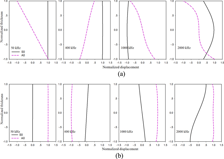
Consider a 1.02 mm aluminum plate bonded with a 6.35 mm PZT actuator. The material properties of the plate are E = 70.0 GPa, ν = 0.3 and ρ = 2700 kg m−3. Figure A.2 presents the across-the-thickness displacement distributions of Lamb waves at four different excitation frequencies. Normalized displacement–thickness curves are shown, and only the S0 mode and the A0 mode are presented.
Figure A.2. Across-the-thickness displacement distributions of Lamb waves at four different excitation frequencies: (a) in-plane displacement, (b) out-of-plane displacement.
Download figure:
Standard image High-resolution image
At a low frequency (50 kHz), the in-plane displacements are constant and linearly distributed across the thickness for the S0 mode and A0 mode, while the out-of-plane displacements are almost zero and constant across the thickness, respectively. Hence, the widely used first-order shear deformation theory or the Mindlin plate theory, in which w is independent of z and the transverse shear deformation and rotary inertia effects are taken into account, is capable of providing accurate predictions of Lamb wave propagation.
At a relatively high frequency (400–1000 kHz), the displacement distributions across the thickness change slightly but are different from the case of the low frequency (50 kHz). The distributions of the in-plane and the out-of-plane displacements across the thickness are, respectively, approximately constant and linear for the S0 mode while linear and almost constant for the A0 mode. It is obvious that the effect of lateral contraction should be taken into account within the first-order shear deformation theory to fully approximate the displacement distribution across the thickness at a relatively high frequency. The plate theory used in the present investigations has taken into account the lateral contraction and can thus provide reasonably accurate results at a relatively high frequency of up to 1000 kHz (or more precisely, up to 1.0 MHz mm). Figure A.2 confirms that the discrepancy of the S0 mode for the 400 kHz case in figure 14 is not mainly due to the linear variation assumption used in the model, but it is attributed without consideration to the interface adhesive layer in the numerical simulations, as reported in [17].
At a much higher frequency (e.g., 2000 kHz), the displacement distributions across the thickness are complicated and are no longer approximately constant or linear. Thus, higher-order plate theories should be used. Wang and Yuan [26] pointed out that, theoretically, it is possible to expand the displacement fields in terms of the thickness coordinate up to any degree. For computational efficiency considerations, however, higher-order plate theories with three orders or less are commonly adopted. Furthermore, it is noticed that the displacement distributions across the thickness are symmetric about the middle plane for the S0 mode and are anti-symmetric for the A0 mode.