
Abstract
In this paper, we present the first implementation of the novel localization relationships, formulated in the recently developed mathematical framework called materials knowledge systems (MKS), into a finite element tool to enable hierarchical multiscale materials modeling. More specifically, the MKS framework was successfully integrated with the commercial finite element (FE) package ABAQUS through a user material subroutine. In this new MKS-FE approach, information is consistently exchanged between the microscale and macroscale levels in a fully coupled manner. The viability and computational advantages of the MKS-FE approach are demonstrated through a simple case study involving the elastic deformation of a component made from a composite material. It will be shown that the MKS-FE approach can be used to accurately capture the microscale spatial distributions of the stress or strain fields at each material point in the macroscale FE model with substantial savings in the computational cost.
Export citation and abstract BibTeX RIS
1. Introduction
A 2006 NSF Report [1] has identified 'the tyranny of scales: the challenge of multiscale modeling and simulation' as one of the core challenges for advances in simulation based engineering science (SBES). This report suggests that the conventional multiscale modeling approaches are incapable of addressing physical phenomena operating across the large range of length scales encountered in the design of advanced materials (∼10 orders of magnitude in spatial length scales are anticipated), and that fundamentally new concepts and approaches are essential to address this challenge. In a more recent report from the National Materials Advisory Board (NMAB) [2], the Committee on Integrated Computational Materials Engineering (ICME) emphasized the importance of multiscale modeling (both spatial and temporal) for the design, development and accelerated insertion of new high-performance materials in emerging advanced technologies. This report further clarifies the anticipated roles of concurrent modeling and hierarchical modeling in multiscale simulations of materials phenomena. While conceding that the goal of multiscale materials modeling is true concurrent modeling (e.g. [3–7]), the report states that for the foreseeable future most multiscale modeling will be accomplished in practice by information passing between stand-alone codes. The latter approach is referred to as hierarchical modeling (e.g. [8–12]) in this paper as it usually entails passing information between constituent disparate length scales.
The main drawback of the hierarchical modeling approach is that it usually employs various simplifying assumptions and therefore trades accuracy for computational speed. On the other hand, the scale-bridging relationships used in hierarchical modeling are better suited for quantitatively capturing the specific influence of any selected microstructure parameter on the macroscale material response of interest. This information is central to the materials design effort [8–11]. Consequently, the hierarchical approach requires the execution of a large number of numerical simulations at each selected length (or time) scale of interest, and establishing the salient structure–property–processing correlations of interest by mining the large number of datasets produced by these simulations. Although this constitutes a significant effort, it is typically a one-time effort. It is generally expected that the overall computational effort involved in setting up hierarchical multiscale models is far smaller than the overall computational effort involved in seeking simultaneous numerical solutions of governing field equations at all length scales of interest in concurrent multiscale modeling, especially when a large number of simulations need to be performed as in the materials design effort.
Another important difference between concurrent multiscale modeling and hierarchical multiscale modeling relates to the direction in which the information flows between the constituent length scales in the problem. Since all governing field equations are solved simultaneously in the concurrent multiscale modeling approach, information flows in both directions between the disparate length scales, albeit at a significant computational cost. In most hierarchical modeling approaches to date, the focus has been in communicating the effective properties to the higher length scales, i.e. on homogenization. Consequently, there is often very little information passed in the opposite direction, i.e. localization. As an example, localization might involve the description of the spatial distribution of the response field of interest (e.g. stress or strain fields) at the microscale for an imposed loading condition at the macroscale. In several materials design problems (for example, in simulating thermo-mechanical processes on materials where there is macroscale heterogeneity in the evolution of the underlying microstructure) localization is just as important as homogenization, if not more important. Furthermore, if localization is addressed with adequate accuracy, it implicitly results in much higher accuracy for homogenization.
The homogenization and localization relationships used in hierarchical multiscale modeling can be significantly improved by employing better measures of the material structure at the lower length scale (referred to as the microstructure in this paper). This is the central idea behind the recently formulated scale-bridging framework called materials knowledge systems (MKS) [13–17]. Building on the established concepts of n-point statistics for the rigorous quantification of the microstructure [11, 18] and the statistical continuum theories developed by Kroner [19, 20], MKS establishes high fidelity microstructure–property–processing relationships that are amenable for bi-directional exchange of information between the constituent hierarchical length scales. In the MKS framework, the localization relationships of interest are expressed as calibrated meta-models that take the form of a simple algebraic series whose terms capture the individual contributions from a hierarchy of local microstructure descriptors. Each term in this series expansion is expressed as a convolution of the appropriate local microstructure descriptor and its corresponding local influence at the microscale. The series expansion in the MKS framework is in complete accordance with the series expansion obtained in the statistical continuum theories developed by Kroner [19, 20]. However, the MKS approach dramatically improves the accuracy of these expressions by calibrating the convolution kernels in these expressions to results from previously validated physics-based models. In a recent work [17], the MKS approach was demonstrated to successfully capture the tails of the microscale stress and strain distributions in composite systems with relatively high contrast, using the higher order terms in the localization relationships. It was also demonstrated that the MKS approach can be applied to problems involving non-linear material behavior such as spinodal decomposition and rigid-plastic deformation [13, 14]. The MKS approach has an analog in the use of Volterra kernels [21, 22] for modeling the dynamic response of nonlinear systems.
This paper describes our first attempt to link the MKS framework with a commercial finite element (FE) code to enable multiscale materials modeling. The merits and limitations of this new MKS-FE approach are critically evaluated. In this initial foray, we have limited the discussion to elastic deformations in a component made from a low-contrast composite material.
2. MKS framework
Generalized composite theories for effective elastic response of heterogeneous materials are well established in the literature, especially for linear properties such as conductivity and elastic stiffness [20, 23–25]. Inherent to these theories is the concept of a scale-bridging localization tensor that relates the local fields of interest at the microscale to the macroscale (typically averaged) fields. For example, the fourth-rank localization tensor for elastic deformation, a, relates the local elastic strain at any location of interest in the microstructure, ε(x), to the macroscale strain imposed on the composite, 〈ε(x)〉, as


In equations (1) and (2), I is the fourth-rank identity tensor, C'(x) is the deviation in the local elastic stiffness at spatial location x with respect to that of a selected reference medium, Γr is a symmetrized derivative of Green's function defined using the elastic properties of the selected reference media, and 〈···〉 brackets denote ensemble averages over representative volume elements (RVEs).
The evaluation of the terms in the series expression in equation (2) requires knowledge of higher order spatial correlations of local states in the microstructure (related to the n-point statistics of the microstructure [18, 20, 26, 27]). Local states are defined as a combination of observable microstructural parameters (such as phase, lattice orientation, composition), and their correlations contain quantitative information regarding their spatial distribution. The series terms in equation (2) correspond to a hierarchy of local spatial statistics of the microstructure. More explicitly, the first 〈···〉 term on the right-hand side of equation (2) captures the contribution to the tensor a(x) from the local state at point x' in the material. In a very similar manner, the second 〈···〉 term in equation (2) reflects the contribution from two local states at points x' and x'', respectively, to a(x).
There exist two main difficulties in the computation of the localization tensor defined in equation (2). The first difficulty stems from the evaluation of the ensemble averages that are in fact convolution integrals whose integrands exhibit singularities (also known as the principal value problem). The second difficulty is that the accuracy of the solutions obtained is quite sensitive to the selection of the reference medium [28]. It should also be noted that the expression of the localization tensor in equation (2) does not lend itself to a scheme where some of the calculations performed for one microstructure may be efficiently carried forward to the calculations for a different microstructure. In other words, any changes in the microstructure would force one to re-evaluate almost all of the terms in the series expansion.
The convolution expressions in equation (2) can be conveniently cast into discrete Fourier transform (DFT) space [29, 30] to allow exploitation of the fast Fourier transform (FFT) algorithms in seeking solutions to the localization relationship (also called Lippmann–Schwinger equation). Indeed, this approach has been explored by many authors in the literature (e.g. [31–35]). However, these approaches continue to require relatively high computational resources because of the iterative schemes employed in the solution methodologies. Although, the approaches described in prior literature are very useful for capturing the intricate details of the microscale response in a single RVE, they are not well suited for addressing inverse problems in materials design (where a very large number of microstructures need to be evaluated and screened) or for conducting practical multi-scale simulations where every material point at the macroscopic level is to be associated with a representative three-dimensional microstructure. In recent papers [13–17], we present a new mathematical framework to cast equation (2) into a computationally efficient, potentially invertible, scale-bridging linkage that is especially suited for multi-scale design and analyses of composite microstructures. These scale-bridging relationships are expected to capture the salient aspects of the microstructure–property linkages at a given length scale, and to communicate them to a higher length scale. It is therefore important to recognize that our approach is not designed for accurately capturing all of the finest details of these linkages, rather it is more suited to provide computationally efficient scale-bridging relations through series expansions that consider higher order statistics of the microstructure. A central element of this new framework is the transformation of the generalized composite theories described in equation (2) into an efficient spectral (Fourier) form that decouples the terms capturing the physics (called influence functions) from the terms capturing the microstructure topology (called microstructure function). We describe below only the final expressions of the MKS approach, and the interested reader is referred to our earlier papers [36, 37] for further details of this transformation.
In the MKS framework, we use the concept of microstructure function [38]. In this description, the three-dimensional spatial domain of the material internal structure is discretized into a uniform grid of spatial cells (or voxels) indexed by s ∈ S. Let |S| denotes the number of spatial cells in the tessellated microstructure domain. The microstructure datasets identify the amount of each local state (e.g. phase identifiers, elemental compositions, crystal lattice orientations) present in each spatial cell. The set of all distinct local states that are possible in a given material system is referred to as the local state space. The local state space is also tessellated into individual bins enumerated by h = 1, 2, ..., H. Following the approach proposed by Adams et al [38], the microstructure function, denoted by
 , is defined as the volume fraction of each distinct local state h in the spatial cell s. Based on this definition of discretized microstructure variable, it is easy to establish the following properties:
where Vh denotes the volume fraction of local state h in the entire microstructure dataset.
Let 〈p〉 denote the macroscale imposed variable (e.g. local stress, strain or strain rate tensors) that needs to be spatially distributed in the microstructure as ps for each spatial cell indexed by s. For many physical quantities of interest, 〈p〉 is indeed equal to the volume-averaged value of ps over the microscale. This is certainly true in the case studies discussed in this paper as they involve only elastic deformations (without initiation of any damage or cracks or the creation of new interfaces by debonding). In the MKS framework, the localization relationship, extended from Kroner's statistical continuum theories [19, 20], captures the local response field in the microstructure using a set of kernels and their convolution with higher order descriptions of the local microstructure. The localization relationship can be expressed as a series sum [13–17]:
where the kernels
 and
and
 are referred to as the first-order and second-order influence coefficients, respectively, which are assumed to be completely independent of the microstructure descriptors
. For multi-scale problems involving elasticity, these influence coefficients are fourth-rank tensors, as shown in equation (4). The influence coefficients capture the contributions of various microstructure features in the neighborhood of the spatial position s to the local response field at that position. The first-order influence coefficients
capture the influence of the placement of the local state h in a spatial location that is t away from the spatial cell of interest denoted by s. Likewise, the second-order influence coefficients
capture the combined effect of placing local states h and h' in spatial cells that are t and t' away, respectively, from the spatial cell of interest s. In this notation, t enumerates the bins in the vector space used to define the neighborhood of the spatial bin of interest [38], which has been tessellated using the same scheme that was used for the spatial domain of the material internal structure, i.e. t ∈ S. It should be noted that the influence coefficients in the localization relationship (equation (4)) are closely related to the Green's function used in other problems [39, 40]. For simplicity, we will limit the considerations in this paper to the first-order influence coefficients. Higher order coefficients have been shown to play an important role in composites with medium to high contrast [17]. A salient feature of the MKS approach is that the influence functions are established such that they are independent of the microstructure topology [13–17]. The multi-scale modeling framework presented here can be easily extended to include the higher order coefficients as needed.
are referred to as the first-order and second-order influence coefficients, respectively, which are assumed to be completely independent of the microstructure descriptors
. For multi-scale problems involving elasticity, these influence coefficients are fourth-rank tensors, as shown in equation (4). The influence coefficients capture the contributions of various microstructure features in the neighborhood of the spatial position s to the local response field at that position. The first-order influence coefficients
capture the influence of the placement of the local state h in a spatial location that is t away from the spatial cell of interest denoted by s. Likewise, the second-order influence coefficients
capture the combined effect of placing local states h and h' in spatial cells that are t and t' away, respectively, from the spatial cell of interest s. In this notation, t enumerates the bins in the vector space used to define the neighborhood of the spatial bin of interest [38], which has been tessellated using the same scheme that was used for the spatial domain of the material internal structure, i.e. t ∈ S. It should be noted that the influence coefficients in the localization relationship (equation (4)) are closely related to the Green's function used in other problems [39, 40]. For simplicity, we will limit the considerations in this paper to the first-order influence coefficients. Higher order coefficients have been shown to play an important role in composites with medium to high contrast [17]. A salient feature of the MKS approach is that the influence functions are established such that they are independent of the microstructure topology [13–17]. The multi-scale modeling framework presented here can be easily extended to include the higher order coefficients as needed.
In prior work [16], we have demonstrated that it is possible to estimate the numerical values of the influence coefficients by calibrating the series expansions of equation (4) to results obtained from micro-mechanics finite element models. We have also shown that equation (4) takes a much simpler form when transformed into the DFT space, where it can be recast as:

where ℑk denotes the DFT operation with respect to the spatial variables s or t, and the superscript star denotes the complex conjugate. Note that the number of coupled first-order coefficients in equation (5) is only H, although the total number of first-order coefficients remains as |S| * H. This simplification is a direct consequence of the well-known convolution properties of DFTs [41]. Because of this dramatic uncoupling of the first-order influence coefficients into smaller sets, it becomes trivial to estimate the values of the influence coefficients
 by calibrating them against results from FE models. It is emphasized here that establishing
is a one-time computational task for a selected composite material system because these coefficients are implicitly assumed to be independent of the morphology of the microstructure. Once the influence coefficients are established for a given composite material system, equation (5) can be used to compute the spatial distribution of the selected response variables of interest for any microstructure dataset.
by calibrating them against results from FE models. It is emphasized here that establishing
is a one-time computational task for a selected composite material system because these coefficients are implicitly assumed to be independent of the morphology of the microstructure. Once the influence coefficients are established for a given composite material system, equation (5) can be used to compute the spatial distribution of the selected response variables of interest for any microstructure dataset.
The procedures for establishing the influence coefficients were discussed in our prior work [13–17]. This was accomplished by calibrating equation (5) to results from FE simulations. More specifically, the influence coefficients were calibrated using delta microstructures on a 21 × 21 × 21 voxel RVE subjected to periodic boundary conditions. A total of six different periodic boundary conditions were used to build the complete MKS database needed for elasticity problems for simulating any arbitrary boundary condition.
It is acknowledged here that identifying the correct boundary conditions in multi-scale problems is an outstanding problem in the field. The reader is referred to [42] for a discussion of this problem. In this work, we have followed the most commonly employed approach in the literature of using periodic boundary conditions, as they are particularly well suited for DFT representations. It is also noted that the basic MKS formulation in equation (4) is not restricted to any set of boundary conditions (i.e. the influence functions can be calibrated to any selected set of boundary conditions); however, the use of periodic boundary allows one to use DFT representations and obtain the highly simplified de-coupled version shown in equation (5). For this reason, we have restricted our attention in this study exclusively to periodic boundary conditions in setting up the MKS framework.
3. Multi-scale simulation using MKS-FE approach
The MKS framework described in the previous section is intended to formulate a multi-scale constitutive description at a material point. As described above, this framework assumes that the hierarchical length scales of interest in the material are sufficiently separated and utilizes periodic boundary conditions at each relevant length scale to address both the homogenization and localization problems. It is noted that for problems where the scales are not well separated, other approaches such as micromechanical finite element methods are better suited for capturing the intricate details of the microscale response. In the MKS-FE approach described in this paper, we aim to use the FE approach for the macroscale analyses (at the component scale) and MKS approach for the microscale analyses. This MKS-FE integration was accomplished through the use of a user material subroutine (UMAT) in the commercial finite element analysis package ABAQUS [43]. In this MKS-FE simulation, each material point in the macroscopic FE model is associated with a representative three-dimensional microstructure at that location. In this novel approach, information is consistently exchanged between the microscale and macroscale in a fully coupled manner. In other words, the MKS approach is used to compute the microscale spatial distribution of the stress and strain fields at each material point in the macroscopic FE model, and the homogenized (volume-averaged) stress field from the microscale is transferred to the macroscale FE analyses at the component scale. Although only the homogenized stress is transferred to the macroscale simulation in the present case study, it is noted that all details of the microscale stress field are available in the MKS approach for upscaling (to the macroscale). This is a particularly valuable aspect of the MKS-FE approach developed in this work.
Let 〈σ〉 and 〈ε〉 denote the macroscale stress and strain tensors defined at an integration point in the FE model. The microscale stress and strain tensors in each spatial cell s are calculated using the MKS approach (equations (4) and (5)) as
where
 represents the fourth-order elasticity tensor for the local state h,
 is the fourth-rank localization tensor and
 denotes the inverse DFT operator that transforms from the Fourier space (k) to the real space (s).
The implementation of UMAT in ABAQUS also requires the computation of the Jacobian defined as
4. Evaluation of the MKS-FE approach
The MKS approach has already been validated in prior work [13–17] for a range of materials phenomena including elastic deformation in multi-phase composites. Our focus here is the critical evaluation of the integrated MKS-FE approach described in this paper. For this purpose, we have compared the microscale stress and strain distributions predicted from the MKS-FE approach with the corresponding predictions from a direct FE simulation with an extremely fine mesh resolution (i.e. a very large number of elements in the FE model) that allows explicit incorporation of the microstructural details. A simple case study involving the elastic bending of a cantilever beam made from a composite material was selected for this evaluation.
Figure 1 illustrates the main features of the MKS-FE and the direct-FE simulations for the elastic bending of a composite cantilever beam. In the MKS-FE model, the cantilever beam is discretized into 637 cuboid-shaped three-dimensional eight-noded solid elements (C3D8) [43]. At each integration point inside each element of the mesh, the microstructure is represented by a spatial domain comprising 9261 (21 × 21 × 21) cubical voxels that are occupied by one of the two different phases colored black and white in figure 1. In this simulation, the macroscale strain tensor provided by ABAQUS at each integration point is used to calculate the microscale strain and stress tensors at each cell in the microstructure using equations (6)–(8). Then, the volume-averaged stress tensor along with the Jacobian matrix is passed up to the macroscale FE analyses (see figure 1(a)).

Figure 1. FE model of the cantilever beam bending problem: (a) a schematic of how the MKS approach is integrated with the FE package ABAQUS in the form of a user material subroutine (UMAT), referred to as MKS-FE approach in this paper, and (b) a direct FE model of the cantilever beam used to validate the MKS-FE approach. Each element in the MKS-FE model shown in (a) is discretized into 21 × 21 × 21 elements in the direct FE model shown in (b). The elements in each 21 × 21 × 21 block of elements are assigned the same 3D microscale structure and local properties as the microscale RVEs used in the MKS-FE model.
Download figure:
Standard imageIn the direct-FE simulation, each element in the MKS-FE model is further discretized into 21 × 21 × 21 elements, as shown in figure 1(b), resulting in a total of 5 899 257 3D solid elements (C3D8). The elements in each 21 × 21 × 21 block of elements are assigned the same 3D microscale structure and local properties as the microscale RVEs used in the MKS-FE simulation, as depicted in figure 1.
5. Results and discussion
A two-phase composite material was selected for this study. The two phases are assumed to exhibit isotropic elastic behavior with Young's moduli of 200 GPa and 300 GPa, respectively. The value of Poisson's ratio is assumed to be 0.3 for both phases. The selection of these values of properties classifies this composite as a low-contrast composite. For higher contrasts, it becomes necessary to include higher order influence coefficients in the MKS approach [17].
In this case study, two different microstructures were selected to validate the MKS-FE approach. The first microstructure was constructed by random placement of the individual phases in the microstructure, as depicted in figure 2(a), and is referred to as the random microstructure in this paper. The random microstructure with its rich diversity of local neighborhoods produces the most heterogeneous microscale stress and strain fields in the composite, and offers an excellent opportunity to validate the MKS-FE approach. The second microstructure is made of rods (or short fibers) placed randomly in the microstructure and oriented along the sample x-direction, as shown in figure 2(b), and is referred to as the rod microstructure in this paper. The volume fraction of both phases in both microstructures was kept about 50%. For simplicity, we assume that the microstructure is the same at each integration point in the MKS-FE model.
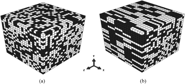
Figure 2. Details of the two different microstructures used to validate the MKS-FE approach: (a) random, (b) rods (or short fibers) oriented along the x-direction.
Download figure:
Standard imageOur goal in this study is to critically validate the MKS-FE approach by comparing the spatially resolved microscale stress or strain fields in the MKS-FE model with the stress or strain fields of the corresponding block in the direct FE model. It is emphasized that our desire here is to validate the spatial distribution of the stress or strain fields at the microscale level using the localization relationship as opposed to just examining the effective stress or strain values of the RVE through any of the homogenization theories. More specifically, elements A and B in figure 1(a) were selected for these comparisons as they represent some of the highest stress locations in the beam.
A meaningful direct comparison of the MKS-FE results with the direct FE results presented a substantial challenge because of a fundamental difference in these models. The mesh used in the MKS-FE model was fairly coarse because a finer mesh would require an even higher level of discretization in the direct FE model (note that each element of the MKS-FE model is further discretized into 9261 elements in the direct FE model). As a result of this coarseness, the MKS-FE results indicated a substantial gradient in the y-direction (i.e. the beam height). Of course, the direct model results also show a similar gradient within the corresponding block of 9261 elements. In order to make a meaningful direct comparison between the MKS-FE results and the direct FE results obtained in this study, it is essential to devise a suitable interpolation scheme for the results obtained from the MKS-FE results. This interpolation scheme is described next.
In the MKS-FE model, each material point is assumed to correspond to a 21 × 21 × 21 microscale RVE. However, the microscale strain (and stress) distributions are output from the simulation only at each of the eight integration points in the C3D8 elements used on this model. The output microscale distributions at the eight integration points were interpolated using linear shape functions consistent with the C3D8 elements to obtain the microscale distributions at spatial locations corresponding to the centroids of each element in the corresponding block of the direct FE model, as shown schematically in figure 3. It is important to recognize that this procedure results in the use of different weights for each of the eight integration points for each selected spatial location. Consequently, we now have 9261 microscale distributions for each element of the MKS-FE model. A composite 21 × 21 × 21 microscale distribution was assembled from this large set by accepting one value from each microscale distribution, as shown in figure 3, and used in the direct comparisons with the results from the direct FE model. As an example, the MKS-FE prediction for the microscale strain tensor in spatial cell s = 100 for element A is taken from the spatial cell s = 100 in the interpolated microscale strain distribution at the corresponding spatial cell (i.e. s = 100) in element A, as shown in figure 3.

Figure 3. Illustration of the interpolation scheme used in this work to compare the microscale spatial strain and stress fields predicted from the MKS-FE approach with the corresponding predictions from the direct FE simulation.
Download figure:
Standard imageFigure 4 shows a comparison of the contour plots for the microscale (εs)11 component of strain for mid-planes through the random microstructure (shown in figure 2(a)) at elements A and B predicted by both the MKS-FE model (using the interpolation scheme described above) and the direct FE model. It is seen that the two predictions are in excellent agreement with each other.
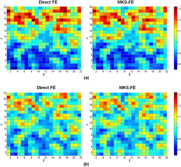
Figure 4. Comparison of contour maps of the local ε11 component of strain (normalized by the macroscopic applied strain) for the mid-plane of the random microstructure (figure 2(a)), calculated using the MKS-FE model against the corresponding predictions from the direct FE model at (a) location A and (b) location B in the cantilever beam model shown in figure 1.
Download figure:
Standard imageFigure 5 compares the frequency distributions of the microscale σ11 component of stress in each phase in the random microstructure at elements A and B in the MKS-FE model with the corresponding frequency distributions of the elements of blocks A and B in the direct FE model. In this figure, the stress distributions from the MKS-FE approach are shown using solid lines, while the stress distributions from the direct FE model are shown using dotted lines. It is seen that the predictions from the MKS-FE method matched very well with the corresponding predictions from the direct FE model. It is also observed that the difference in the stress distributions between the two approaches is slightly higher at element A compared with element B, especially in the tails of the distributions. The reasons for this difference are discussed in more detail below. However, it is worth noting that the accuracy of the MKS-FE model for capturing the effective stress continues to be very high. For example, the values of the averaged stress component 〈σ11〉 were predicted by the MKS-FE model were 145.9 MPa and 134.8 MPa at elements A and B, respectively; the corresponding values predicted by the direct FE model were 144.9 MPa and 134.3 MPa, respectively.

Figure 5. Comparison of the microscale stress distributions predicted from the MKS-FE model against the corresponding predictions from the direct FE model at (a) location A and (b) location B in the cantilever beam model shown in figure 1. Results are for the random microstructure shown in figure 2(a).
Download figure:
Standard imageIt should be noted that the predictions from the MKS-FE approach are obtained with very minimal computational effort. Specifically, for the case study discussed here, the direct FE simulation involving about 6 million elements required 15 h when using 64 processors on a supercomputer (using National Center for Supercomputing Applications, NCSA, UIUC, IL), whereas the MKS-FE simulation took only 55 s on a standard desktop computer (2.6 GHz CPU and 4 GB RAM). It is therefore clear that there is tremendous gain in computational efficiency in using the MKS approach for conducting practical multi-scale FE simulations.
In order to better compare the predictions from the MKS-FE approach with the predictions from the direct FE model, we define an average difference measure as
where the superscripts DFE and MFE indicate that the predictions were made using the direct FE and MKS-FE methods, respectively. Based on the above definition, the difference measures for ε11 between the two predictions in elements A and B for the random microstructure were 3.1% and 1.3%, respectively. However, we have previously evaluated the same influence coefficients without coupling the MKS with FE tool, by comparing the microscale strain fields in a single RVE predicted by the MKS against the corresponding predictions from a microscale FE model subjected to periodic boundary conditions, and found that the maximum error was only 1% [16]. It is therefore seen that the difference between the MKS-FE and direct FE predictions presented here is higher than the inherent error expected in the MKS formulation (from calibration of the influence coefficients). We attribute this increased value of difference to two main reasons. (i) As noted earlier, the coarse discretization of the MKS-FE mesh results in a significant macroscale gradient (along the beam height in the y-direction) within the element, which appears to contribute to this difference. (ii) The boundary conditions in the direct FE model are significantly different compared with the periodic boundary conditions implicit in the MKS formulation. Both these points are discussed in more detail next.
In order to confirm that the coarse discretization of the MKS-FE mesh contributes to the observed difference, we produced a slightly coarser mesh with 325 elements. The corresponding direct FE mesh had ∼3 million elements. Repeating the same analyses described earlier, it was noted that the difference between the MKS-FE and the direct FE predictions in elements A and B increased from 3.1% and 1.3% to 5.2% and 2.3%, respectively. This observation suggests that the coarseness of the MKS-FE mesh does indeed contribute to the observed difference between MKS-FE and the direct FE simulations presented earlier. In this study, we were limited to the coarse mesh shown in figure 1 because we aimed to match each element in the MKS-FE mesh to a microstructure of 21 × 21 × 21 elements in the direct FE mesh. Constraints on available computing resources did not permit a finer mesh in the MKS-FE simulation. In addition, it is observed that the difference between the MKS-FE and direct FE approaches at the fixed end of the cantilever beam (location A in figure 1), which is known to experience the highest stress fields, is always higher than that at any other location in the cantilever beam. This clearly suggests that more discretizaton is needed near the fixed end to decrease the effect of strain gradient and therefore improve the agreement between the two models.
The fact that the boundary conditions implied in the MKS formulation (i.e. periodic boundary conditions) are substantially different from the boundary conditions imposed on each block of elements of interest in the direct FE does contribute to some of the observed differences between the two predictions discussed earlier. As noted earlier, the difference is highest for the elements at the edge of the MKS-FE mesh, especially the elements whose nodes have an external nodal force. However, we strongly believe that this difference is largely due to the fact that the microstructure in the direct FE simulations was represented by a fairly small RVE. In reality, we expect a substantial difference between the macro- and micro-length scales. Due to limitations on the available computational resources, we were not able to accommodate a much larger RVE that would more accurately reflect the actual length scales involved. Based on the numerous simulations performed we are confident that a higher discretization of the microscale RVE would reduce the observed difference between the two predictions discussed here. This assertion is strongly supported by the observation that a direct comparison between the two predictions (i.e. between a specific spatial cell in the microscale in the MKS-FE simulation and the corresponding element in the direct FE simulation) shows that the differences mostly arise in the boundaries of the microscale RVE.
The predictions of the MKS-FE model and the direct FE model were also compared for the rod microstructure shown in figure 2(b). Because the random and the rod microstructures are distinctly different from each other, this comparison attests the versatility of the MKS-FE approach for a broad range of potential microstructure topologies. Note that the influence coefficients
of the MKS approach have been shown to be independent of the microstructure topology in prior studies [13–17]. In other words, the same set of influence coefficients were used for both microstructure topologies. The microscale distributions of the σ11 component of stress in each phase in the rod microstructure at elements A and B in both the MKS-FE and direct FE models are compared against each other in figure 6. The effective 〈σ11〉 stress values calculated using the MKS-FE approach at elements A and B were 149.4 MPa and 137.83 MPa, respectively, while the effective 〈σ11〉 stress values computed using the direct FE approach at blocks A and B were 148.3 MPa and 137.6 MPa, respectively. Furthermore, we compare in figure 7 the spatial distributions of the local (σs)11 component of stress for a mid-plane through the rod microstructure at element B from both the MKS-FE and direct FE models. It is seen once again that the two predictions are once again in excellent agreement with each other for the case of rod microstructure. The average differences between the MKS-FE and direct FE predictions of the local strain components at locations A and B for the rod microstructure were approximately 3.1% and 1.2%, respectively. This result demonstrates the versatility of the MKS-FE approach in its broad applicability to a wide range of microstructure topologies.

Figure 6. Comparison of the microscale stress distributions predicted from the MKS-FE model against the corresponding predictions from the direct FE model at (a) location A and (b) location B in the cantilever beam model shown in figure 1. Results are for the rod microstructure shown in figure 2(b).
Download figure:
Standard image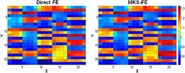
Figure 7. Comparison of contour maps of the local σ11 component of stress (normalized by the macroscopic effective stress component 〈σ11〉) for the mid-plane of a 3D rod microstructure (figure 2(b)), calculated using the MKS-FE against the corresponding predictions from the direct FE model at location B in the cantilever beam model shown in figure 1.
Download figure:
Standard image6. Conclusions
This work demonstrates the first implementation of the localization relationships formulated in the recently developed MKS framework into a finite element tool to enable multiscale materials modeling. The MKS approach was integrated with the commercial finite element package ABAQUS through a user material subroutine. The new MKS-FE approach was critically validated on a case study involving the elastic bending of a cantilever beam made from a composite material by including the microstructure features at each material point in the FE model. In this novel approach, information is consistently exchanged between the microscale and macroscale in a fully coupled manner.
In this work, the microscale stress and strain distributions predicted from the MKS-FE approach were compared with the corresponding predictions from a direct FE simulation with an extremely fine mesh resolution that allows explicit incorporation of the microstructural details. It is found that the MKS-FE approach accurately captures the microscale stress and strain fields in the microstructure at a dramatically reduced computational cost. It is also shown that the mesh densities and boundary conditions in the MKS-FE and direct FE models contribute to the observed difference between these models.
Acknowledgments
This work was partially supported by the National Center for Supercomputing Applications under DMR110025. The authors gratefully acknowledge financial support received for this work from NSF Grant CMS-0727931.