
Abstract
Solid-state magnetic cooling near room temperature has recently gained a prominent position among alternative cooling technologies that are deemed to have higher energy efficiency compared to vapour compression. This prospect has surged a rapid growth of the area of magnetocaloric materials. Although several breakthroughs were achieved, the extensive study revealed a number of challenges in the effective deployment of the magnetic refrigerants. This review focuses on fundamentally and technologically relevant aspects of the cooling with magnetocaloric materials. A critical evaluation of magnetic refrigerants and progress made in improvement of their performance is provided. Future development trends in the field of materials for the solid state cooling are highlighted.
Export citation and abstract BibTeX RIS
1. Introduction
In recent years magnetocaloric materials have gained increasing interest as materials for application in alternative cooling and refrigeration systems. The rising interest is related to the fact that air conditioning and refrigeration account for at least 15% of energy consumed in residential and commercial buildings (Goetzler et al 2009, Preuß et al 2011). The majority of sold cooling units are based on the vapour compression technology (DOE 2010), yet the technology is mature—it has been in service for over 100 years—and foreseen efficiency improvements have an incremental character (Park et al 2015). Whereas the best commercial vapour compressors reach about 40% of Carnot efficiency, magnetic cooling system studies predict Carnot efficiency of more than 60%, i.e. substantial energy efficiency gains compared to the conventional vapour compression are expected (Zimm et al 1998, Engelbrecht et al 2007, Gschneidner and Pecharsky 2008). Along with the prospect of higher efficiency, magnetic cooling offers a lower environmental impact, as no hazardous fluids and only a few movable parts (low noise pollution) are used.
The magnetocaloric effect (MCE) was discovered in nickel almost a century ago by Weiss and Piccard (1917) (for the history of the discovery see Smith (2013)). Using general thermodynamics and Langevin's function Debye (1926) predicted the possibility of cooling by adiabatic demagnetisation to temperatures close to absolute zero. Giauque and MacDougall (1933) were the first to demonstrate a practical implementation of the magnetocaloric effect: by adiabatic demagnetisation of a paramagnetic salt, gadolinium sulfate octahydrate, they were able to attain temperatures of about two tenths of a Kelvin. The turning point towards magnetic refrigeration near room temperature was the demonstration of a regenerative thermodynamic cycle in gadolinium, a metal with a sizable MCE at the Curie transition at about 295 K (Brown 1976). A significant achievement showing that magnetic cooling can compete with vapour compression technology was the demonstration of a successful proof-of-principle cooling unit employing Gd as magnetic refrigerant in 1997 (Gschneidner and Pecharsky 2008). In the same year, a giant MCE due to a first order magnetostructural transition has been reported in Gd5Si2Ge2 by Pecharsky and Gschneidner (1997a). This has triggered substantial research activities resulting in the observation of the giant MCE in other material classes (Tegus et al 2002, Fujita et al 2003, Gschneidner et al 2005, Krenke et al 2005, Brück 2008). A recent milestone was the demonstration of an industrial prototype wine cooler refrigerated by a magnetic heat pump in 2015 (ChemistryViews 2016). Nevertheless, as of now the magnetic refrigeration is not commercialised. In order for this technology to disrupt the existing vapour compression dominated market, considerable research activity needs to continue in terms of both providing the fundamental knowledge on how to design the most effective magnetocaloric materials and how to engineer efficient solid-state magnetic cooling systems.
It should be emphasised that adequate characterisation of potential magnetic refrigerant materials is crucial in the assessment of their applicability in magnetic cooling. One lesson to be taken is that the misinterpretation of the order of the transition, such as that occurred on the discovery of ternary intermetallic Gd5(Si,Ge)4 compounds (Holtzberg et al 1967), might lead to failing of taking account of compounds with a potentially large MCE. Since the MCE determination can be intricate, especially in magnetocaloric materials experiencing a first order transition, it was decided to dedicate a part of this review to characterisation techniques.
A number of reviews on various magnetocaloric material classes and their properties has been published in the recent years (Tishin and Spichkin 2003, Gschneidner et al 2005, Brück 2008, Franco et al 2012). Here, a progress in understanding the properties of the magnetocaloric materials crucial for applications is reported with an emphasis on material design. On the basis of thermodynamic considerations, differentiation of first order transitions into two different types according to the relation of the thermal energy to the height of the energy barrier between magnetic states below and above the transition point is proposed. The review discusses materials potentially interesting for near room temperature cooling and magnetic refrigerants already employed in prototypes. Moreover, magnetocaloric materials in thin film form that can serve as model systems for the development of new solid state cooling concepts are reviewed.
2. Magnetocaloric effect and magnetic heat pumping
Temperature change under a magnetic field variation is the manifestation of the magnetocaloric effect. The role of the magnetic field H is to influence the arrangement of electron spins in a solid and, thus, change its magnetic entropy Smag, which is a consequence of the largely configurational character of the latter. By following the effect of the field on a solid represented in figure 1(a) in terms of the spin and lattice systems, the essence of the magnetic cooling becomes vivid. The application of the magnetic field leads to the alignment of spins and reduces the magnetic entropy Smag. Under adiabatic conditions (the total entropy S = const), the reduction in Smag is compensated from other sources within the material. By recalling that the total entropy also contains a phonon term Sph (Wohlfarth 1980), it is apparent that the compensation can be brought about by an increase in Sph, i.e. by intensified lattice vibration. This situation is schematically illustrated by a largely exaggerated phonon wave in figure 1(a), step I. As a result of the increased lattice vibration the temperature rises. The evolved heat is removed from the system to the environment, also called bath (step II). On thermal isolation of the solid from the environment and removal of the magnetic field, the spins randomise causing an increase in Smag and the corresponding reduction in Sph. This step leading to the temperature reduction received the name 'adiabatic demagnetisation' (step III, figure 1(a)). Adiabatic demagnetisation is a one-shot process. The magnetic cooling by the adiabatic method is thus intentionally shown in figure 1(a) as an incomplete cycle, because due to the inevitable heat flow from the environment the end temperature is always the temperature of the bath. It was only several years later since the adiabatic demagnetisation demonstration by Giauque and MacDougall (1933), when a continuous refrigeration using the MCE has been introduced by Heer et al (1954).
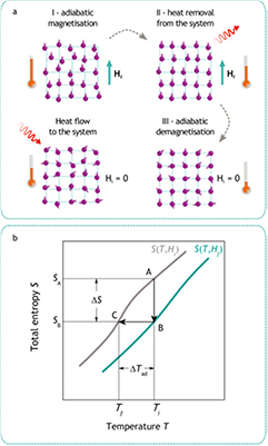
Figure 1. Thermodynamics of the magnetic cooling: (a) the spin and phonon systems and (b) the entropy of a solid. The solid is a paramagnet or a ferromagnet near the Curie temperature.
Download figure:
Standard image High-resolution imageFigure 1(b) illustrates the thermodynamic equivalent of the model discussed above in terms of the entropy state equation, not as a thermodynamic cooling cycle. The temperature T dependence of the total entropy S(T, H) is shown in the magnetic fields Hi and Hf being the initial (often zero) and final fields, respectively, so that Hi < Hf. In the process AB, the field is applied and the heat evolved as a result of Smag decrease is rejected isothermally to the bath at temperature Ti. In the process BC, the adiabatic (isentropic) demagnetisation cools the solid from temperature Ti to Tf. The above discussion is valid for a ferromagnet near the Curie temperature or a paramagnet, where the application of the magnetic field leads to the reduction of the magnetic part of the entropy. In certain materials, e.g. in magnetic Heusler alloys and magnetically anisotropic materials, the application of the magnetic field may lead to the reduction of the net magnetisation and as a consequence a so-called inverse MCE is observed, i.e. the material cools on field application (Manosa et al 2013).
The knowledge of the total entropy S(T, H) is sufficient to completely describe the magnetocaloric effect (note that since the magnetic cooling is carried out at essentially a constant pressure, pressure is omitted in the expression for S). Taking into account the 2nd and 3rd law of thermodynamics and the fact that a measurement can only be performed above absolute zero, we arrive at the following expression for the entropy:

where Cp is the heat capacity, S0 is a constant associated with the number of states of possible nuclear spin orientations (Reif 1985) and T0 is the starting temperature of the measurement.
In many applications, only entropy difference ΔS is of importance. In magnetocaloric applications, one refers to the entropy change ΔS as a difference between the entropy at a field Hi and Hf. S0 is independent of external parameters (Fliessbach 1995); therefore, making use of the result  one obtains the relation for the entropy change:

where  . By using experimental heat capacity measurements and by numerical integration of equation (2), the entropy change can be obtained.
In terms of MCE schematics in figure 1(b), the entropy change is an isothermal difference  given by

In the isentropic process ( ) corresponding to the adiabatic magnetisation (
 ), a further parameter can be defined—the adiabatic temperature change

where  is the temperature at the point C (figure 1(b));
  emphasizes the dependence of ΔTad on the specific start temperature of the adiabatic process. Likewise, the specific field values Hi and Hf are crucial in the determination of ΔS and ΔTad. Since these scale with the field as Hn, where n < 1 (Oesterreicher and Parker 1984, Kuz'min et al 2011, Lyubina et al 2011), ΔS and ΔTad will assume different values depending on whether the change is from 0–1 T or from 1–2 T, irrespective of the same field difference
  . Usually, Hi = 0 and by referring simply to a field difference
  this fact is tacitly assumed. We will not do this exercise here, but note that analytical derivation of the results in equations (3) and (4) is also possible (Pecharsky and Gschneidner 2001a).
ΔS and ΔTad are used as an alternative to S(T, H) for the complete description of MCE. Applicability of a particular magnetocaloric material for cooling purposes requires the knowledge of further material parameters (section 5).
As discussed above, the magnetocaloric effect enables heat pumping, i.e. the movement of the heat from a reservoir at temperature Tcold to a reservoir at Thot (Tcold < Thot), when a device is subjected to a work. Clearly, a heat pump can operate as refrigerator, when the heat is picked up from the cold space and expelled to the environment (Thot) or in the heating mode, where the heat from the environment (Tcold) is moved to the interior space (Thot). Thermodynamics states that it is possible to proceed in the reverse way and extract heat from a heat reservoir and convert it into macroscopic work (Reif 1985). Such a concept was introduced by Stefan (1889) and patented in the form of a thermomagnetic generator by Tesla (1890) and Edison (1892), for the detailed history see a paper by Smith (2013). Thermomagnetic energy generation employs the decrease of the magnetisation of a ferromagnet at the Curie temperature Tc to produce work (Kirol and Mills 1984), but is unrelated to the magnetocaloric effect. Nevertheless, materials with a rapidly changing magnetisation that are considered for magnetic cooling can also be suitable candidates for the thermomagnetic generation (Dung et al 2011) and are deemed to be able to compete with thermoelectric generation (Vuarnoz et al 2012). A proof-of-principle thermomagnetic generation device employing (Mn,Fe)2(P,As) as active material was recently demonstrated by Christiaanse and Brück (2014).
The adiabatic demagnetisation is not suitable for heat pumping near room temperature, since in most magnetocaloric materials ΔTad is too small (<8 K, see section 6) to attain a useful temperature span  and thermal loads are too large to be carried by a direct thermal contact (Brown 1976). The so-called magnetic regeneration method allows to attain a temperature span
  significantly larger than ΔTad (Brown 1976). A concept that is used for magnetic heat pumping nowadays is that of an active magnetic regenerator (AMR), where the magnetocaloric material acts simultaneously as refrigerant and regenerator (Barclay 1982, Barclay and Steyert 1982), hence the name of the magnetic refrigerant as often used in the literature.
AMR consists essentially of a magnetic regenerator containing a magnetocaloric material, a magnetic field source and accessories which control the device (figure 2). As magnetic field source a permanent magnet is preferred, since in this case only a motor that delivers a field variation is required. This sets a limit on the maximum attainable field to below 2 T. A review of various permanent magnet designs can be found in Bjørk et al (2010b). The heat exchange fluid is pushed back and forth through the regenerator by a pump and control valves are used to regulate the flow. The magnetocaloric material in the regenerator bed is shaped in a way to allow the fluid flow; possible geometries include powders, plates or a bulk material with pores or channels. If particles are used to form a layered (i.e. several Tc) magnetic refrigerant bed, these must be fixed, e.g. by an epoxy, in order to prevent particle intermixing during the AMR operation and the resultant disturbance of the temperature profile.
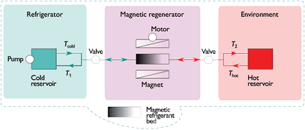
Figure 2. Active magnetic regenerator.
Download figure:
Standard image High-resolution imageCooling using the AMR cycle involves four distinct steps (Jacobs et al 2014). First, the fluid is stagnant and the magnetic refrigerant is heated by the application of a magnetic field. Next, while the field is still on, the fluid at a temperature Tcold is pumped through the refrigerant bed from the cold to hot end and leaves the regenerator at a higher temperature T2; the heat is exhausted to the surroundings and temperature reduces to Thot < T2. Next, the magnetic field is removed, the refrigerant cools and the flow is reversed; the fluid passing through the refrigerant bed cools from Thot to T1. Finally, the fluid leaving the regenerator is revolved through the cold heat exchanger, accepts heat from the refrigerator and leaves it at temperature Tcold, by this keeping the refrigerator at a lower temperature. The flow and the corresponding fluid temperatures are shown schematically in figure 2.
Most of the reported AMR employ gadolinium as magnetic refrigerant and can provide a cooling power of 100–1000 W, common for household appliances (Zimm et al 1998, 2006, Yu et al 2010, Rowe 2011, Tura and Rowe 2011, Engelbrecht et al 2012). A magnetic refrigerator employing 1.5 kg of La(Fe,Si)13Hy spherical particles with six different Curie temperatures was recently shown to be able to provide a high cooling power of about 2000 W at  (Jacobs et al 2014). The electrical coefficient of performance (COP) of about 2 was measured for this large-scale device. Ultra-high efficiency cooling units based on the vapour compression technology can provide COP of up to 5.8 (Brown and Domanski 2014). It is obvious that there is a need for improvement of this parameter in order for the magnetic refrigeration to hold the promise of the improved energy efficiency. General considerations for the design of an efficient AMR and AMR thermodynamics are discussed by Engelbrecht et al (2012) and Burdyny et al (2014). A distinct advantage of the AMR systems is the ambient pressure operation, which offers additional possibility to improve thermodynamic efficiency by optimisation of heat exchangers which, in contrast to vapour compression systems, do not have to contain high pressure gas. Also on the side of the magnetic refrigerants improvements are urgently sought after. Besides technological considerations, the magnetocaloric effect is of fundamental significance, since the appearance of the MCE is a result of complex interactions in the solid state. Therefore, characterisation of the magnetocaloric effect as well as revealing the fundamental interplay between magnetism and thermodynamics plays a vital role in the understanding and control of the magnetocaloric materials and ultimately their performance improvement.
3. Magnetic phase transitions and classification of magnetocaloric materials
The order of the phase transition is a key parameter in the evaluation of magnetocaloric materials. The magnetic phase transitions in the magnetocaloric materials are distinguished into first and second order. The knowledge of the transition type is indispensable in modelling and prediction of the material performance and in developing strategies that help to overcome known hindrances typical for the transition type.
Figure 3 presents schematically the difference in the first and second order transition types according to the Ehrenfest classification, which defines the transition order by the order of the derivative after which the thermodynamic potential  exhibits a discontinuity.
  here represents the Gibbs potential (Castellano 2003). The entropy S, magnetisation M and volume V are the first derivatives of
  and at second order transitions these are changing smoothly with temperature and show no discontinuity at the transition point Tc (figure 3). The heat capacity near Tc has the λ-anomaly. ΔS curves have a caret shape; the peak maximum ΔSmax grows with the field according to a law Hn. In the mean field model, n = 2/3 (Oesterreicher and Parker 1984), whereas in materials not following the mean field description n can be around 0.75 (Franco et al 2006a).
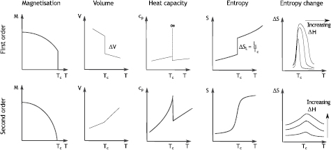
Figure 3. Magnetisation M, volume V, heat capacity Cp, entropy S and entropy change ▵S in dependence on the field change ▵H at first and second order magnetic phase transitions.
Download figure:
Standard image High-resolution imageMaterials with a first order transition are much more intriguing, as these show a giant magnetocaloric effect; the name 'giant' stresses the fact that the entropy change in first order materials is significantly larger than that in second order materials, such as a benchmark material Gd. The underlying mechanism behind giant MCE differs from material to material and can be due to a magnetic transition coinciding with a structural one with or without symmetry change (Pecharsky and Gschneidner 1997a, Dung et al 2011, Lyubina 2011), spin reorientation (Pique et al 1996) or ferromagnetic (FM) to antiferromagnetic (AFM) transition (Tu et al 1969, Nikitin et al 1990). A discontinuity in the volume ΔV, magnetisation ΔM and entropy  , where Si and Sf are the entropies of initial and final states, respectively (figure 3) has major implications for the material performance as magnetic refrigerant and determination of the MCE, which will be discussed in the following sections. In contrast to materials with the second order transition, the ΔS curve in first order-type materials moves not vertically, but aslant with the field as a consequence of the temperature dependence of the critical field of the transition (Lyubina et al 2008, Caron et al 2009, Morrison et al 2009).
Thermodynamic models describing temperature and field dependence of ΔS and ΔTad are an indispensable tool for modelling of the performance and design of the refrigerator device, where a particular set of parameters, not always available in the form of experimental data, is required. The knowledge of the MCE scaling behaviour is also of fundamental importance, as it can be used in the search and design of magnetocaloric materials with improved properties. A common approach in the description of second order materials is the use of the Landau expansion (Romanov and Silin 1997, Amaral and Amaral 2004, Kuz'min 2008, Kuz'min et al 2011, Lyubina et al 2011) or the Arrott–Noakes equation of state (Franco and Conde 2010).
In the Landau theory, it is assumed that the thermodynamic potential  can be expanded in terms of the order parameter ξ close to the transition point (Landau and Lifshitz 1980). In magnetic materials, the magnetisation M is taken as the order parameter and the magnetic part of the thermodynamic potential
  without external magnetic field can be written as
where a, b and c are material parameters and  is a term of zeroth order; we limit ourselves to the first three terms of the power row. At thermal equilibrium
  and the Landau's theory of the second order transitions (we consider the first two terms of the expansion only) yields the following expression for the entropy change (Kuz'min and Richter 2009)

where Mi and Mf are the magnetisation in the initial (zero) and in final magnetic fields, respectively.
The entropy change obtained from the Arrott–Noakes equation of state has the following form (Franco and Conde 2010)
where β and γ are the critical exponents. Franco et al (2008) showed that by fitting the magnetisation data and making use of equation (7), the ΔS shape can be predicted in a broad temperature range around the Curie temperature. For the description of the MCE in materials with the first order transition the Preisach model was shown to be useful (Basso et al 2005, von Moos et al 2015). In the framework of the molecular mean field model incorporating Bean–Rodbell magnetovolume coupling Belo et al (2012) have established a scaling behaviour of the maximum entropy change with the Curie temperature  , which was found to hold for both, second and first order transitions.
The strong dependence of the exchange energy on the lattice volume were shown by Bean and Rodbell (1962) to be responsible for the appearance of the first order transition. Models based on the Bean and Rodbell model that consider the magnetic, crystal lattice and electron contributions to the free energy were developed for the description of the magnetocaloric effect in materials with first order transitions (de Oliveira and von Ranke 2010, Basso 2011). Further models used to describe the magnetocaloric effect include molecular field approximation (Amaral et al 2007), Monte-Carlo method (Nóbrega et al 2006, Buchelnikov et al 2011) and first principles calculation (Paudyal et al 2006, Kuz'min and Richter 2007, Liu and Altounian 2009, Roy et al 2016). It should be noted that first principles calculations can be instrumental in finding materials with properties favourable for magnetic cooling applications (see section 5.3).
Making use of the expansion in equation (5), one can also derive the maximum entropy change ΔSmax as a function of the field (Lyubina et al 2011)

where A and B are material constants and the parameter H0 relates to the distribution of Curie temperatures in the material. The same field dependence is observed for the maximum ΔTad (Kuz'min et al 2011). Strictly speaking, equation (8) should only be valid for materials experiencing a second order transition, since the relation was derived on the basis of the Landau's theory of second-order phase transitions. However, Lyubina et al (2011) showed that equation (8) can also be useful in describing the entropy change of materials with the first order of particular types. It is valid for materials with a non-uniform (continuous) magnetic first order phase transition, such as that observed in materials with a distribution of the particle or crystallite size or other inhomogeneity (Lyubina et al 2010) and in materials with the gradual transition from first to second order (Lyubina et al 2011, Morrison and Cohen 2014). It has been recognised that only materials that follow the relation in equation (8) have a chance of finding application in magnetic cooling.
So we set out to find out the thermodynamic characteristics of such materials useful for the application. Above the Curie temperature, the condition  and
and  in equation (5) corresponds to the condition for the observation of the first order transition, as opposed to the second order transition, where
  and
and  (Grazhdankina 1969). From the form of equation (5) we note that for
  ,
,  ,
,  and
and  the function
  has two minima at
  and at a finite value of the magnetisation
  ; the two minima are separated by an energy barrier U (Yamada 1993). The condition for the appearance of the first order transition with the corresponding minima can also be derived using a microscopic model in the mean field approximation (Alho et al 2012). The dependence
  for such first order transition from the para- to ferromagnetic state is schematically shown in figure 4. For the particular case of
  shown in figure 4, the FM state at
  is metastable. Overcoming the energy barrier between the two minima is a thermally activated process, which has a characteristic energy
  (
( is the Boltzmann constant) of about 25 meV near room temperature. When this condition is not fulfilled, the state at
  can be induced by an external magnetic field; the transition occurs non-quasistatically at a critical field Hmi. There will be a difference in Hmi in two directions, i.e. the hysteresis ΔHhys will arise. This hysteresis is proportional to the energy barrier,
  .
.
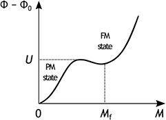
Figure 4. Magnetic part of the thermodynamic potential  as a function of the magnetisation M for a hypothetical refrigerant undergoing a first order transition from the paramagnetic (PM) to the ferromagnetic (FM) state.
Download figure:
Standard image High-resolution imageIn the magnetocaloric materials, a generally linear trend is observed in the relation between hysteresis and the prominent first order characteristics of the phase transition, latent heat (Morrison and Cohen 2014)

Two groups of first order materials can be further distinguished: one material group, such as Gd5Si2Ge2, CoMnSi, Mn1.95SbCr0.05, NiMnInCr, has a significantly larger hysteresis ΔHhys compared to another material group (e.g. LaFe13−xSix for x < 1.8, manganites exhibiting a first order transition) at the same value of the latent heat L (Morrison and Cohen 2014).
Taking into account the above observations and thermodynamics, we can now differentiate first order transitions into two different types according to the relation of the height of the energy barrier U between magnetic states below and above the transition point to the thermal energy  . A transition of the first type, we will call it strong first order transitions, is characterised by a high energy barrier
  . This transition type is often observed in materials with a strong magnetostructural coupling (e.g. Gd5Si2Ge2). A transition of the second type, we name it weak first order transition, has an energy barrier U comparable to the thermal energy
  . The weak first order transitions are typical for materials with a gradual departure from first- to second order transformation (e.g. LaFe13−xSix). Strong first order materials show a significantly larger hysteresis compared to materials with the weak first order transition.
Itinerant magnet systems, such LaFe13−xSix and (Mn,Fe)2P-type alloys are prominent examples of magnetocaloric materials with the weak first order transition. The transition from first to second order is gradual and the hysteresis associated with the first order transition is low—a very favourable characteristic allowing a greater flexibility in tuning the MCE and lowering hysteresis. The energy barrier between different magnetic states in the LaFe13−xSix alloys is typically below 150 meV/f.u. (Kuz'min and Richter 2007); this value is expected to be even lower in the MnFeSixP1−x compounds (Roy et al 2016). These energy barriers are comparable to the thermal energy near 300 K. The effect of the thermal energy is to smear out the transition, therefore, the transition in weak first order materials appears to be smooth (Lyubina et al 2009b, Brück et al 2012), as opposed to the textbook example with a distinct discontinuity in the magnetisation ΔM (see figures 3, 5 and 6). Nevertheless, the transition is clearly first order, as indicated by the presence of the latent heat L at the transition (Morrison and Cohen 2014).
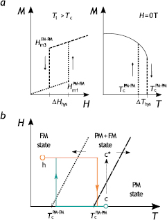
Figure 5. Hysteresis at a first order magnetic phase transition. (a) Magnetisation M in dependence on the magnetic field H (temperature T) sweep with characteristic critical fields (temperatures) of the transition  (
( ) and field hysteresis
  (thermal hysteresis
  ). (b) The corresponding magnetic phase diagram constructed with the use of
  and
and  .
.
Download figure:
Standard image High-resolution image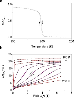
Figure 6. Experimentally observed magnetisation M in melt-spun LaFe11.6Si1.4 showing a weak first order transition in dependence on (a) temperature and (b) magnetic field. M(T) was measured in the field of 10 mT. The arrows indicate the direction of the temperature and magnetic field sweep.
Download figure:
Standard image High-resolution imageIn terms of heat capacity behaviour (Morrison and Cohen 2014), these two first order transition types show distinctly different behaviour (figure 7). At the strong first order transition the heat capacity  peak shifts with increasing magnetic field, but its height is less affected by the magnetic field;
  dependence shows a sharp step and its height only weakly depends on temperature with the corresponding weak temperature dependence of the latent heat (figures 7(a)–(c)). At the weak first order transition the functions
  ,
,  and
and  are in the form of a broad peak and are strongly sensitive to temperature and magnetic field; the magnitude of the latent heat decreases with increasing field (figures 7(d)–(f)). There exist materials (e.g. CoMnSi exhibiting a FM-AFM transition), where a combination of the two characteristics is observed (Morrison and Cohen 2014).
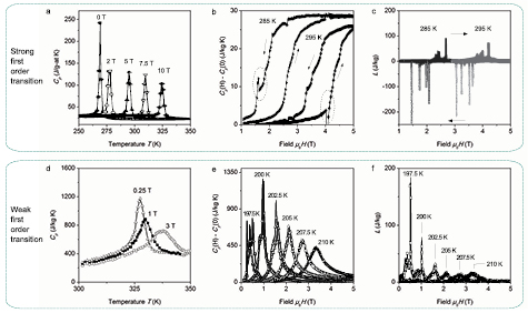
Figure 7. Classification of first order transition types in magnetocaloric materials in terms of temperature dependence of the heat capacity Cp, field dependence of the heat capacity Cp(H) and latent heat L. (a) Cp(T) of homogenised Gd5Si2Ge2 in various magnetic fields. (b) Change in heat capacity of single crystal Gd5Si2Ge2 at 285 and 295 K; the dotted circles highlight (irreproducible) artefacts due to latent heat. (c) Latent heat of single crystal Gd5Si2Ge2 at 285 and 295 K; sharp spikes in L indicate multiple nucleation of the ferromagnetic phase over a range of critical fields. The arrows indicate the direction of the magnetic field sweep. (d) Cp(T) of melt-spun LaFe11.6Si1.4H1.6 in various magnetic fields. (e) Change in heat capacity of bulk homogenised LaFe11.44Si1.56 at different temperatures and (f) the corresponding latent heat of bulk homogenised LaFe11.44Si1.56. Cp(0) is the heat capacity in zero magnetic field. The data is compiled from Pecharsky et al (2003), Morrison and Cohen (2014) and own data.
Download figure:
Standard image High-resolution imageAs apparent from figure 7(a), the thermal energy smears the strong first order transition as well, albeit to a much lesser extent compared to the weak first order transition. As a result, the phase transition in strong first order materials also occurs in a finite temperature and field range and, although very sharp, the heat capacity has a finite value (no singularity, compare to figure 3); this value only weakly depends on the field.
It should be emphasised that the existence of the weak first order transition follows from the thermodynamics and should not be mistaken with a broadened (sequential or continuous) first order transition. The distribution in the transition temperatures (broadening) can arise as a result of inhomogeneous microstructure, impurities, crystal defects, stray fields and local difference in strain (Pecharsky et al 2003, Morrison et al 2009, Lyubina et al 2010, Lovell et al 2015). Inhomogeneity and local difference in strain smear out the weak first order transition additionally to the thermal energy (Lyubina et al 2010). This effect is also observed in materials with the strong first order transition, such as Gd5(SixGe1−x)4 alloys (Pecharsky et al 2003): in an arc-melted inhomogeneous Gd5Si2Ge2 alloy containing an impurity phase, the heat capacity behaviour in increasing magnetic fields resembles that of weak first order materials shown in figure 7(d), i.e. the field not only shifts the transition to higher temperatures, but also smears out the  peak significantly. This is in contrast to a homogenised Gd5Si2Ge2 alloy, where the
  behaviour remains clearly of strong first order character.
4. Magnetocaloric effect measurement
4.1. Direct measurement
Although the direct measurement of the MCE is straightforward, the lack of commercial equipment impedes the widespread use of this technique. A recent review of home built equipment can be found in Smith et al (2012).
To measure ΔTad one needs to ensure adiabatic conditions and provide means for a magnetic field variation and temperature measurement. Thermocouple is commonly used to measure temperature directly (Dan'kov et al 1997, Lyubina et al 2009a, 2010, Skokov et al 2009); indirect temperature measurements can also be employed (Otowski et al 1993, Christensen et al 2010). According to the way the magnetic field variation is achieved, one distinguishes ΔTad measurement systems where the source of the magnetic field is stationary and a sample is moved relatively to this source (Bjørk et al 2010a, Yibole et al 2014) and systems where the magnetic field is varied in time and the sample position is fixed (Dan'kov et al 1997, Lyubina et al 2009a, 2010, Skokov et al 2009, Kuz'min et al 2011, Morrison et al 2012c, Ghorbani Zavareh et al 2015). Adiabatic conditions require the avoidance of heat exchange between a sample and environment for the duration of the measurement. Along with a good thermal insulation a fast magnetic field change is essential; this can be realised by moving permanent magnets (Lyubina et al 2009a, 2010, Skokov et al 2009) or in pulsed fields (Dan'kov et al 1997, Ghorbani Zavareh et al 2015). Exemplarily, ΔTad for a single crystal Gd and bulk LaFe11.6Si1.4 alloy measured in a device (Lyubina et al 2009a, 2010, Skokov et al 2009, Kuz'min et al 2011, Morrison et al 2012c), where the magnetic field is provided by a rotating Halbach-type permanent magnet assembly and temperature is recorded by a thermocouple, is shown in figure 8. The use of vacuum and heat shields combined with a field variation rate in the order of 1 T s−1 ensures adiabaticity. In Gd, where no field or thermal hysteresis is expected to occur, essentially no difference in ΔTad(H) on the application and removal of the magnetic field is apparent (figure 8(a)). In contrast, substantial field hysteresis at and above Tc (191 K and 195 K in figure 8(c)) and thermal (Lyubina et al 2010) hysteresis is observed for the bulk LaFe11.6Si1.4 alloy, which is caused by dynamic processes within the solid (Lovell et al 2015).
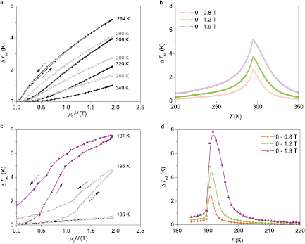
Figure 8. Directly measured adiabatic temperature change ▵Tad in dependence on the magnetic field sweep and temperature; the rate of the field change is 1.8 T s−1. (a) and (b) Single crystal Gd, Tc = 295 K and (c) and (d) bulk LaFe11.6Si1.4 alloy, Tc ≈ 191 K. Single crystal Gd was provided by K A Gschneidner, Jr.
Download figure:
Standard image High-resolution imageDifferential scanning calorimetery (DSC) enables a direct entropy change ΔS measurement. Basso et al (2008, 2010) reported direct ΔS measurements in a home built Peltier cells heat flux DSC, where an electromagnet is used as magnetic field source. As in a commercial DSC, reference materials are used either for the determination of the calibration constant connecting the measured voltage to the heat flux or the time constant governing the kinetics. The DSC signal is due to a sum of the heat capacity and latent heat. When operated under isothermal conditions, the DSC measures a heat flux due to the change of the applied magnetic field and the induced entropy change ΔS can be directly measured.
4.2. Indirect measurement
The so-called indirect measurement of the MCE is a widely adopted technique in which either the heat capacity is measured in a calorimeter or magnetisation is measured in a magnetometer and the MCE is subsequently computed from the acquired data.
4.2.1. Heat capacity.
The calculation of the entropy S and entropy change ΔS in materials experiencing a second order transition is performed using equations (1) and (2) by numerical integration of Cp(H, T) data. Even though the transitions we are interested in are taking place around room temperature, it is important to start recording Cp(H, T) at the lowest possible temperature (typically between 2 and 5 K) to keep the error arising due to the entropy term S0 low (Lyubina 2016). The accuracy of the MCE calculation from Cp data was studied in detail by Pecharsky and Gschneidner (1999a, 1999b).
The first order characteristics of the phase transition, latent heat (equation (9)), needs to be accounted for in the calculation of the entropy from Cp data in materials with the first order transition. Clearly, the latent heat cannot be determined by the integration of the heat capacity in materials with a very sharp first order magnetic phase transition and a singularity in Cp at the transition point (figure 3), such as that observed in ultra-pure and homogeneous Dy metal (Pecharsky et al 1996). The infinitely large heat capacity makes the accurate determination of the height of the  jump impossible.
In most materials, the phase transition occurs in a finite temperature range and, as a result, although sharp, the heat capacity has a finite value (figure 7). Regardless of the first order transition type (strong, weak or inhomogeneity broadened), the latent heat must be captured appropriately in order to correctly determine the MCE (Pecharsky and Gschneidner 1999b, Morrison et al 2012a). Therefore, special procedures for the independent determination of L should be adopted.
Pecharsky et al (1996) proposed a method for capturing the latent heat at sharp first order transitions that can be used in a heat pulse calorimetry, a technique often used in both home-built and in commercial equipment operating near and below room temperature. In accordance with the thermodynamics, if the material experiences a first order transformation, the latent heat L will effectively change the amount of heat supplied to it by the calorimeter  (
( , m is the sample mass) and, thus, will introduce uncertainty in the measurement. The method consists in the application of heat pulses
  with a different amplitude and recording temperature rise and decay
  (Pecharsky et al 1996). The heat pulse resulting in
  allows the precise determination of the latent heat of the transformation. The corresponding entropy
  should then be added above and below the transition point into the entropy function in equation (1) and the entropy is obtained as

S0 is neglected here. The separate measurement of the latent heat can also be realised by a temperature modulated (micro)calorimetry technique (Morrison et al 2012a, Morrison and Cohen 2014).
4.2.2. Magnetometry.
Calculation of the MCE using calorimetry requires time-consuming and non-trivial Cp measurements. The MCE can alternatively be calculated using magnetometry data; this method is often employed due to its simplicity and effectiveness in terms of reduced data collection time and accessibility of the magnetometry equipment.
Integration of the Maxwell relations (Reif 1985) yields the entropy change that is related to the magnetisation M(T, H) as

Since equation (11) is obtained from the free energy, thermodynamics demands that the states in the initial field Hi and final field Hf are equilibrium states. It is further assumed that the magnetisation M(T, H) has a derivative at the transition point  , i.e. it does not have a jump discontinuity.
At second order transitions, both conditions are fulfilled and the entropy change ΔS is readily calculated by numerical integration of equation (11), if isofield magnetisation curves  or isotherms
  used to build
  are known. Often, isothermal magnetisation is recorded due to a shorter data collection time and well defined lower integration limit Hi (usually zero). In the isofield measurements, recording
  in zero field is connected to a larger uncertainty. The equivalency of both measurements was demonstrated by Morrison et al (2012c).
If open magnetic circuit magnetometry is employed, correction for demagnetising effects is required for the determination of the internal magnetic field

where Happl is the applied field and N is the demagnetising factor. The latter can only be neglected in thin flakes and films with M in the plane or in needles with M along the long axis.
As discussed in the preceding section, in the majority of the first order materials the phase transition occurs in a finite temperature range and, thus, the derivative  exists. This is also the case in ultra-pure and homogeneous materials (Chernyshov et al 2005). However, the condition of the equilibrium can be violated under particular measurement conditions. In magnetocaloric material families showing a field induced metamagnetic or magnetostructural transition, the paramagnetic (PM) state is generally the equilibrium phase above Tc and in H = 0 (Pecharsky and Gschneidner 1997a, Gschneidner et al 2005, Brück 2008, Lyubina et al 2009b, Dung et al 2012). The equilibrium state below Tc or in sufficiently high magnetic fields above Tc is the ferromagnetic state. When the transition occurs in a finite temperature range, a mixture of the PM and FM phases is observed; note that at each particular temperature only a certain PM/FM fraction is an equilibrium fraction. A frequently employed measurement protocol is a 'continuous' cooling (heating), during which an M(H)T curve is recorded at a given temperature and a subsequent M(H)T is recorded at a lower (higher) temperature (Caron et al 2009, Bratko et al 2012). Magnetic field sweep (zero → maximum field → zero) at a particular temperature may not always return the material to the equilibrium (e.g. PM in zero field), but some part of the sample can transform to a non-equilibrium state (e.g. FM) in the magnetic field and remain in this state in zero field. The PM/FM phase fraction will thus deviate from the equilibrium. The reason for the observation of this behaviour is a non-zero hysteresis at the transition (figure 5). Considerable errors arise as a result of the equilibrium condition violation (Caron et al 2009). In extreme cases, failure to take this effect into account can lead to a 'colossal entropy change overestimation' yielding unphysically large ΔS (Bratko et al 2012).
In first order materials, where a field sweep during magnetisation measurements induces a non-equilibrium state, another procedure for recording M(H)T data is required. The essence of the method lies in 'resetting' the material to its equilibrium state by either heating well above—point c in figure 5(b) (or cooling well below—point h in figure 5(b)) the temperature of the transition. The solid thus attains equilibrium before the next isotherm is recorded (Caron et al 2009, Bratko et al 2012). It should be appreciated, however, that the formation of inhomogeneous magnetisation states (Amaral and Amaral 2010) and magnetically induced reorientation in martensitic Heusler alloys (Niemann et al 2014) can be another source of spurious effects and need to be eliminated in the calculation of ΔS.
It should be emphasised that the magnetometry technique allows the calculation of the total entropy change. Statements found in the literature that only the magnetic part of the entropy is captured by magnetisation measurements are erroneous; although the magnetic field merely influences Smag, the change in Smag obviously induces a variation in other relevant entropy terms (here, Sph). Provided the equation (11) applicability conditions are not violated, the entropy change obtained from heat capacity resembles that from magnetometry (see e.g. Manosa et al 2009, Morrison et al 2010, Bratko et al 2012).
The integration of the Maxwell relation and the use of equation (1) yields the following expression for the adiabatic temperature change:
As is apparent from equation (13), the ΔTad determination using magnetometry data requires the knowledge of Cp(T, H) additionally to M(T, H). The strong temperature and field dependence of the Cp(T, H) function (figure 7) does not allow to treat the heat capacity as a constant and exclude it from the integral in equation (13) (Pecharsky and Gschneidner 1999a). On the other hand, the availability of Cp data (and hence S data) in fields Hi and Hf makes the use of equation (13) obsolete, as simply equation (4) can be applied for ΔTad calculation. Nevertheless, it is appreciated that if the Cp(T, H) data is available only for a limited number of fields, equation (13) can be useful in the calculation of missing entropies S(T, Hi) and S(T, Hf) and the corresponding ΔTad determination (Pecharsky and Gschneidner 1999a).
Clausius–Clapeyron equation (Reif 1985) is an alternative method that can be used to obtain the entropy change at first order transitions:
It correlates the equilibrium line slope  in the magnetic phase diagram (figure 5(b)) to the discontinuity in entropy
  and magnetisation
  and assumes equal chemical potentials of the phases at the transition point. Since the transition between the two magnetic states must essentially be complete (which is ensured by the application of a sufficiently high magnetic field), equation (14) gives the limit of the entropy change achievable in a particular material at this transition (see e.g. Giguère et al 1999, Casanova et al 2002, Fujita et al 2013a). In practice, the magnetisation change occurs in a finite magnetic field range and not at a single H (figure 6). ΔM is as a result often underestimated (Amaral and Amaral 2010).
5. Properties of magnetic refrigerants
In the evaluation of the suitability of materials as magnetic refrigerants, magnetic and non-magnetic properties should be considered. Along with the assessment of specific material properties, assessment of the economic and environmental merits (precursor/material costs, manufacturing costs, potential health hazards) is equally important. In the following, material properties relevant for magnetic cooling application will be discussed.
5.1. Cooling efficiency
To justify the technology switch from vapour compression to magnetic refrigeration, ever higher performance of magnetic cooling devices must be demonstrated. In this respect, a large MCE in the magnetic refrigerant is a prerequisite for being potentially able to provide a large cooling power and high efficiency. The entropy change ΔS is a measure of the material's cooling power; adequate ΔTad is required to move the heat. MCE increase with the magnetic field change (see equations (11) and (13)) is limited, since the available magnetic field provided by permanent magnets is below 2 T and in high magnetic fields the MCE does not grow unlimitedly, but eventually saturates (Tishin 1990, Lyubina et al 2011). Therefore, the maximisation of MCE should be achieved through an increase of  (equations (11) and (13)).
The magnetisation derivative is maximised at magnetic phase transitions. The derivative  at first order transitions is significantly larger compared to that at second order transitions (see the magnetisation curves versus temperature in figure 3). The steep magnetisation variation leads to the observation of the giant MCE (Nikitin et al 1990, Pecharsky and Gschneidner 1997a); the latter is commonly observed in the magnetocaloric materials with a coupled magnetic and structural transformation either with or without symmetry change (figure 9). The entropy change ΔS of giant MCE materials is limited to a narrower temperature range compared to materials with a second order transition, resulting in a considerably higher ΔSmax. Figure 10 shows ΔS for a family of LaFe13−xSix alloys that depending on the composition can exhibit a weak first or second order PM to FM transition; the giant MCE material, LaFe11.6Si1.4, possesses ΔSmax a factor of three larger compared to that of Gd.

Figure 9. Schematic crystallographic and magnetic phases above and below the first order transition temperature in various magnetocaloric materials in zero magnetic field (except Gd showing the second order transition). For Gd, T < Tc corresponds to the temperature range between 294 and 232 K, i.e. prior to the onset of spin reorientation.
Download figure:
Standard image High-resolution image
Figure 10. Entropy change ▵S in LaFe13−xSix for a field change 0–1.5 T calculated using equation (11). Data for La(Fe,Mn,Si)13Hz (commercial name CV 310H by Vacuumschmelze) is for a field change of 1.6 T and is courtesy of Barcza and Katter (2015). For comparison, ▵S of Gd in a field change of 0–1.5 T is provided.
Download figure:
Standard image High-resolution imageIt should be emphasised that for the ease of ΔS comparison in various materials and from the engineering point of view, it is advisable to provide ΔS in volumetric, J m−3 K−1, and not in gravimetric units, J kg−1 K−1 (Lyubina et al 2009b, Gschneidner et al 2005). The conversion between the units requires the knowledge of the material density.
The use of a single figure-of-merit reflecting ΔS and ΔTad for a particular magnetocaloric material could provide a convenient means for comparison and assessment of different refrigerant materials. Magnetic refrigerant capacity in the form suggested by Wood and Potter (1985),  , assumes a uniform temperature across the magnetic refrigerant bed (a condition violated in AMR) and equal entropy change at the cold and hot ends,
  . No limitations are posed on ΔTad, allowing it to be unacceptably small. Likewise, from the knowledge of the relative cooling power (RCPΔS) alone, defined as ΔS(T) peak area or as a product of ΔSmax and the full-width-at-half maximum (FWHM) (Gschneidner and Pecharsky 2000, Lyubina et al 2009b), no conclusion can be made, whether cooling can be performed with this material. This is because a large RCPΔS does not necessarily imply availability of a sufficient ΔTad; note the additional heat capacity term in equation (13) compared to equation (11) (Pecharsky and Gschneidner 2006).
The minimum requirement for ΔTad is device specific. Engelbrecht and Bahl (2010) demonstrated that cooling can cease when ΔTad drops below 2 K. Based on this result, one can introduce a figure-of-merit parameter useful for an engineer, RCPΔS|ΔTad > 2 K, defined as an area of the ΔS peak limited to a temperature range, where ΔTad is above 2 K, ( ) (see figure 11 for a graphical visualisation):


Figure 11. Determination of RCP▵S|▵Tad > 2 K from the ▵S(T) diagram. The relative cooling power with respect to the entropy change ▵S is determined as the area below the ▵S(T) curve only in the temperature range ▵Ts = T2 − T1, where in the corresponding adiabatic temperature change ▵Tad(T) ⩾ 2 K.
Download figure:
Standard image High-resolution imageRelative cooling power determined in this manner for different families of magnetocaloric materials is summarised in figure 12. It is apparent that in a single material bed regenerator, Gd by far outperforms not only material families with a second order transition, but also materials experiencing the first order transition. In some material families, such as amorphous Fe78B12Cr8Ce1–5 and Heusler alloys Ni50Mn34In16 and Ni50Mn36Co1Sn13 (Khovaylo et al 2010, data not included in figure 12) the (cyclic) adiabatic temperature change is below 2 K in a field change of up to 2 T and consequently the relative cooling capacity RCPΔS|ΔTad > 2 K is null.
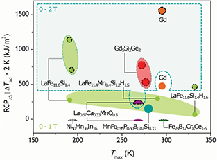
Figure 12. Relative cooling power for different families of magnetocaloric materials RCP▵S|▵Tad > 2 K, defined as a product of ▵Smax and FWHM of the ▵S peak limited to the temperature range, where ▵Tad is above 2 K. The values are provided for a field change of 0–1 T and 0–2 T. The values are computed from data published by Pecharsky et al (2003), Lin et al (2006), Khovaylo et al (2010), Lyubina et al (2010), Law et al (2011), Morrison et al (2012c), Guillou et al (2014b) and Lyubina (2016), except for LaFe11.6Si1.4, LaFe11.6Si1.4H1.6 and Ni50Mn34In16 that are computed from own data. In amorphous Fe78B12Cr8Ce1–5 and Ni50Mn34In16, RCP▵S|▵Tad > 2 K is null in a field change of 1 and 2 T, since ▵Tad is below 2 K for the both field variations.
Download figure:
Standard image High-resolution imageThe MCE in magnetic refrigerants can be influenced by the microstructure. Figure 13 illustrates the effect of microstructure on the entropy change for alloys of the LaFe13−xSix family with a first order transition. The largest entropy change is observed in bulk microcrystalline alloy. The introduction of porosity leads to the removal of constraints imposed by grain boundaries and as a consequence ΔS is decreased by about 30% in porous alloys consisting of cold-pressed powders with surface area moment mean particle size Lm of 225 µm (Lyubina et al 2010, Lyubina 2011). Reduction of the internal strain (constraints), distribution of transition temperatures as well as material degradation due to defects and surface oxidation (Moore et al 2009, Lyubina et al 2010, 2012b, Radulov et al 2015) are discussed in relation to the reduction of the MCE on further decrease of the particle size (figure 13). A dramatic drop of the magnetocaloric effect is observed on reducing the crystallite size to the nanometer range (figure 13). In LaFe13−xSix, the reduction of the grain size to 70 nm and to 40 nm gradually weakens the first order transition and ΔSmax drops by 40% and 60% compared to the microcrystalline counterpart, respectively (Lyubina 2011). The lattice microstrain is on the similar level ( ≈ 0.13–0.15%) for both nanocrystalline materials. Thus, the gradual transition to the second-order regime may be mainly ascribed to the grain size reduction. This behaviour can be a manifestation of random anisotropy effects, when the exchange energy starts to balance the anisotropy energy yielding a so-called intergrain exchange coupling (Skomski 2003). The exchange length, a characteristic length below which atomic exchange interactions dominate magnetostatic fields, is ~10 nm in low magnetocrystalline anisotropy materials, such as LaFe13−xSix. It determines, for example, the transition from a particular magnetisation rotation regime and the grain size below which the hysteresis loops of two-phase magnets appear single-phase-like (Skomski 2003). Apparently, the reduction of the crystallite size in first-order materials to the range comparable to the exchange length weakens magnetostructural coupling in first-order materials and leads to the overall MCE reduction. Similar effects were observed in Gd5(SixGe1−x)4 alloys experiencing a first order coupled magnetostructural transition (do Couto et al 2011, Pires et al 2015). The authors did not report the grain sizes of the ball milled Gd5(SixGe1−x)4 materials explicitly, but the presented x-ray diffraction patterns indicate their nanocrystalline nature. Also in materials with a second order transition the magnetocaloric effect is reduced on decreasing the crystallite size to the nanoscale. For example, crystallite size reduction to the nanometer regime in Gd leads to a sizable drop of ΔS (Mathew et al 2010). Thus, nanostructuring has a detrimental effect on the size of the magnetocaloric effect.

Figure 13. The maximum entropy change ▵Smax in a magnetic field change of 0–2 T for LaFe11.6Si1.4 alloys with different microstructure. ▵Smax for porous microcrystalline LaFe11.6Si1.4 alloy synthesised by pressing of the pulverised bulk alloy is shown as a function of surface area moment mean particle size Lm. ▵Smax for nanocrystalline LaFe11.6Si1.4 alloy prepared by mechanical ball milling at liquid nitrogen temperature is shown as a function of the crystallite size  . The ▵Smax value for bulk microcrystalline LaFe11.6Si1.4 (induction melted and homogenised) is marked for comparison. The data is compiled from Lyubina (2011) and Lyubina et al (2012b).
Download figure:
Standard image High-resolution image5.2. Operation temperature range
To overcome the limitation of a narrow temperature span  and correspondingly lower RCPΔS|ΔTad > 2 K provided by a single (first order) magnetocaloric material, a graded regenerator bed comprising materials with different Curie temperature is employed (Russek et al 2010). Variation of the material composition with the aim of Tc tuning should preferably be performed in a way allowing to retain the large cooling capacity. Exemplarily, specific stoichiometry variation in MnxFe1.95−xP1−ySiy does not change the transition type and potentially a constant and large ΔS is obtainable in
  (figure 14, Dung et al 2011). The condition of the constant ΔS is of utmost importance for the AMR performance (Engelbrecht and Bahl 2010). For engineering a magnetic refrigerant bed containing multiple Tc materials, it is furthermore desirable to have a sufficient and constant adiabatic temperature change along the regenerator length. The AMR performance in dependence on the temperature profile ΔTad(T) along the regenerator, where T is the material's temperature, was studied by Smaili and Chahine (1998), who showed that any monotonically increasing ΔTad(T) can provide adequate regenerator performance. 'Excessive' ΔTad shifts the operating temperature of a neighbouring material from its optimum and thus can reduce the overall efficiency of the refrigerator (Russek et al 2016).
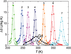
Figure 14. Example of stoichiometry variation that can be used to obtain essentially constant entropy change ▵S in a broad temperature span. ▵S of MnxFe1.95−xP1−ySiy (1: x = 1.34, y = 0.46; 2: x = 1.32, y = 0.48; 3: x = 1.30, y = 0.50; 4: x = 1.28, y = 0.52; 5: x = 1.24, y = 0.54; 6: x = 0.66, y = 0.34; 7: x = 0.66, y = 0.37) and benchmark Gd is shown for a field change of 0–1 T (open symbols) and 0–2 T (solid symbols) (From Dung et al 2011, copyright 2011. This material is reproduced with permission of John Wiley & Sons, Inc.).
Download figure:
Standard image High-resolution image5.3. Hysteresis
Hysteresis is observed both at field induced and temperature induced first order transitions (figure 5) and is detrimental for refrigerator operation. Figure 5(a) shows schematically the hysteresis in the field and temperature driven first order transitions with characteristic transition fields/temperatures and hysteresis widths,  and
and  . Hysteresis can be mapped in the (H, T)-plane by, for instance, extracting the field of the transition
  from the M(H) isotherms at a temperature Ti and constructing a phase equilibrium line
  (figure 5(b)). In materials with the hysteresis, two phase equilibrium lines exist; the first line corresponds to the transition from a high-temperature (e.g. PM, austenite) to a low-temperature (e.g. FM, martensite) phase and the second one corresponds to the reverse transition. In the time independent or static process, the influence of the field and temperature on the transition are equivalent. It is apparent from figure 5(b) that the following relation between the thermal and field hysteresis can be established

Thus, the knowledge of the thermal hysteresis width  and the shift of the transition temperature with the field
  or its inverse value
  allows one to determine the amplitude of the field hysteresis
  . For an ideal first order transition, the adiabatic temperature change can be approximated with the use of equations (11), (13) and (14)

provided the field  is large enough to complete the transformation (Pecharsky and Gschneidner 2006). Note that cooling will cease as soon as
  becomes comparable or exceeds the magnetic field change
  . The same result is obtained on examination of the RCP (Kuz'min and Richter 2007). Obviously, magnetocaloric materials with a large
  or in other words, a steep
  or a small rate of the Tc shift with field and large
  , cannot be good refrigerants. If one follows the transition along the path c → c*, one notices that the lowest field hysteresis is obtained when the width
  and slope of the phase equilibrium line
  are small (figure 5).
Materials with the strong first order transition have a large hysteresis. Exemplarily,  for Gd5Si2Ge2 (table 1),
  in FeRh and
  for Ni50Mn36Co1Sn13 (Basso et al 2012). If the application in the cyclic AMR process is considered, the extremely large hysteresis (especially in the latter case) would require unacceptably high magnetic fields to induce the transformation. In contrast, materials with the weak first order transition are characterised by a much lower hysteresis, e.g.
  for LaFe13−xSix and
  for MnFeSixP1−x-type compounds (table 1). Clearly, only materials with the weak first order transition are attractive for heat pumping applications. We recall that the field dependence of the MCE in these materials follows the form of equation (8).
Table 1. Properties of the magnetocaloric materials with strong and weak first order transitions: the peak temperature of the ▵S curve (Tmax), the gravimetric and volumetric maximum entropy change (▵Smax) in a field change μ0▵H = (0–1) T, the discontinuity of the lattice constants (▵a/a and ▵c/c) and discontinuity in volume (▵V/V), the thermal (▵Thys) and field (▵Hhys) hysteresis and the thermal conductivity (κ) at 300 K.
| Material | Tmax (K) | −ΔSmax (kJ m−3 K−1) | −ΔSmax (J kg−1 K−1) | Lattice discontinuity (%) |  (T) (T) |
ΔThys (K) | κ (W K−1 m−1) | Reference | ||
|---|---|---|---|---|---|---|---|---|---|---|
| ▵a/a | ▵c/c | ▵V/V | ||||||||
| Gd5Si2Ge2 (homogenised) | 272 | 68 | 12 | −0.9 | 0.2 | 0.4 | 1.5–2 | 10 | 5.2 | Morellon et al (1998), Pecharsky and Gschneidner (2001a), Pecharsky et al (2003) and Fujieda et al (2004) |
| LaFe11.6Si1.4 (bulk) | 196 | 147 | 22 | 1.09 | 1.09 | 1.09 | 0.5 | 2.3 | 9.1 | Fujieda et al (2004), Lyubina et al (2009b) and Lyubina (2011, 2016) |
| LaFe11.6Si1.4 (porous and {melt-spun}) | 196 | 76{68} | 11{10} | 1.09 |
1.09 |
1.09 |
0.1 | 0.5 | 2.7–5.0 | Lyubina (2011, 2016), Lyubina et al (2012b) and Radulov et al (2015) |
| Mn1.25Fe0.7P0.5Si0.5 | 274 | 57 | 9 | −0.79 | 1.86 | 0.26 | 21(5.7) |
75(20) |
Brück (2008) and Guillou et al (2014a, 2014b) | |
| MnFe0.95P0.582Si0.34B0.078 | 289 | 57 | 9 | −0.73 | 1.57 | 0.09 | ≈0.1 | 2.5 | Guillou et al (2014a) | |
| MnFe0.95P0.595Si0.3B0.075 | 281 | 62 | 9.8 | ⩽0.05 | 0.4 | 1.6 | Guillou et al (2014b) | |||
| Ni50Mn36Co1Sn13 | 281 |
−110 |
−13.8 |
11 | 16.5 | Khovaylo et al (2010) | ||||
| Ni53.3Mn20.1Ga26.6 | 320 |
220 |
27.6 |
7 | 5.2 | 15.6 | Abhyankar et al (2010) and Basso et al (2012) | |||
| La0.67Ca0.33MnO3 | 268 |
42.8 |
6.9 |
≈0.1 | 5 | 2.0–2.5 | Radaelli et al (1995), Lin et al (2006) and Turcaud et al (2013) | |||
| Fe–Rh | 313–320 | −123.2 | −12.5 | 0.27 | 0.27 | 0.27 | ≈1 | ≈10 | Nikitin et al (1990), Annaorazov et al (1996), Stern-Taulats et al (2014) and Chirkova et al (2015) | |
aLattice expansion accommodated by pores. bThe values in brackets correspond to 2nd cooling, see Brück (2008). cμ0▵H = 2 T. dμ0▵H = 1.2 T.
The mechanism for the appearance of the hysteresis can be of intrinsic and extrinsic origin. The intrinsic hysteresis stems from the fundamental characteristics of the first order transition, the latent heat L (Landau and Lifshitz 1980). The transition can proceed hysteresis-free only in a quasi-static regime (section 3). In the dynamic transition regime, the evolution of the latent heat will move the equilibrium in the endothermic or exothermic process direction depending on the direction of the temperature (or field) sweep. This will lead to the appearance of the intrinsic (i.e. thermodynamically governed) hysteresis. Intrinsic hysteresis is low in materials with the weak first order transition (section 3), as free energy profiles F(M) of such materials have very low energy barriers U comparable to the thermal energy (Yamada and Terao 2002, Kuz'min and Richter 2007, Lyubina et al 2008, Dung et al 2011, Roy et al 2016).
The underlying reason for the appearance of the extrinsic hysteresis is material microstructure and transition kinetics. In first order materials, the transition involves a structural (symmetry or/and lattice constant) change, which, in turn, is responsible for the onset of the magnetism (Bean and Rodbell 1962, Grazhdankina 1969, Yamada 1993). Microstructural features, such as crystallite size and shape, size distribution, porosity, secondary phases, inhomogeneity and strain, change the path along which this structural change actually occurs. A subtle deviation in the transition mechanism suffices to bring about a dramatic variation in the critical temperature/field of the coupled first order phase transition and consequently can bring about a substantial hysteresis (Bean and Rodbell 1962, Grazhdankina 1969).
Since most of the magnetic refrigerants are polycrystalline materials, one of the reasons for the observation of the large extrinsic hysteresis is the large volume change ΔV/V (Fujita et al 2001, Lyubina 2011) or anisotropic expansion (Morellon et al 1998, Yabuta et al 2006) of the crystallites at the first-order transition constrained by neighbouring grains (Lyubina et al 2010, Guillou et al 2014a). Table 1 summarises the lattice discontinuity for various magnetocaloric material families. It is apparent that there is a correlation between the width of the hysteresis and the lattice parameter discontinuities (Dung et al 2012).
Weakening of the first order transition by compositional modification is a common method for the reduction of the hysteresis (Provenzano et al 2004, Lyubina et al 2009b, Guillou et al 2015), but the resultant entropy change can be significantly lower. It is more attractive to retain the first order transition, but at the same time reduce the extrinsic hysteresis. Lyubina et al (2010) demonstrated that in the materials with a large ΔV/V, microstructure modification can provide significant reduction in the extrinsic hysteresis, e.g. by accommodation of the lattice expansion by the introduction of porosity (see bulk and porous LaFe11.6Si1.4 in table 1). Corresponding ΔSmax and  reduction (Lyubina 2011, figure 13) can be mitigated by adjusting the degree of porosity or by embedding magnetocaloric materials in a ductile matrix, e.g. polymer, copper and silver (Lyubina et al 2012b, Turcaud et al 2013, Radulov et al 2015). Specific shaping of the magnetocaloric materials resulting in inhomogeneous magnetisation states was also shown to be useful for noticeable hysteresis reduction (Lovell et al 2015).
A magnetic refrigerator operates in the dynamic regime with a frequency limit f ~ 100 Hz (Kuz'min 2007). Note that practically achievable frequencies are currently <10 Hz, i.e. well below this theoretical value (Tura and Rowe 2011, Engelbrecht et al 2012, Jacobs et al 2014). Since the AMR cooling power is a product of the relative cooling power of the magnetocaloric material RCPΔS|ΔTad > 2 K and f, increasing the operation frequency could provide an attractive means for overall efficiency improvement. For this, low field hysteresis and fast kinetics of the transition are essential. Generally, magnetic isotherms M(H) expand with increasing frequency, i.e.  increases (figure 15, Lovell et al 2015). This flaring is caused by (i) the temperature variation in the material due to the magnetocaloric effect and (ii) poor thermal conductance between the material and surroundings. For the overview of further mechanisms leading to the increase of the hysteresis in magnetic materials in general (e.g. dynamic losses) the reader is referred to a book by Bertotti (1998). Improved thermal linkage and reduction of the magnetocaloric material thickness can significantly reduce the hysteresis arising at high magnetic field rates (Moore et al 2009, Kuepferling et al 2013, Lovell et al 2015). The latent heat generation and dissipation at the boundary between phases involved in the transformation (intrinsic effect) also plays an important role in determining the transition rate (Yako et al 2011, Fujita and Yako 2013, Fujita et al 2013b). Specific microstructure design and the introduction of a second phase (Lyubina et al 2012b) can be used to mitigate this effect.

Figure 15. Flaring of the magnetisation isotherm with increasing the field change rate  during the field driven first order transformation in bulk LaFe11.6Si1.4. The isotherm is measured at 194.5 K; the Curie temperature is Tc = 191 K (adapted from Lovell et al (2015)).
Download figure:
Standard image High-resolution image5.4. Non-magnetic properties: thermal conductivity, workability and stability
The design of the AMR requires anisotropic thermal transport properties of the magnetic refrigerants (Nielsen and Engelbrecht 2012). The thermal conductivity κ along the fluid flow should be low in order not to disturb the temperature gradient between the cold and hot side; the heat exchange transverse to the flow should be, on the other hand, very efficient. While very large anisotropy is observed in layered materials, such as graphite having the ratio of κ in the direction parallel and perpendicular to the c-axis of ~102–103, the thermal transport anisotropy in most materials is significantly lower (Slack 1961). The thermal conductivity of the known magnetocaloric materials is the range of 2–16 W m−1 K−1 at 300 K without any significant anisotropy (table 1). The thermal conductivity can to some extent be varied using synthetic routes and deploying various refrigerant bed geometries (Oezcan et al 2014). Bulk (low porosity) materials show expectedly a higher thermal conductivity. Improvement of thermal transport in higher porosity materials can be achieved by the introduction of a second component (Lyubina et al 2012b, Turcaud et al 2013, Radulov et al 2015). In composites containing a high conductivity material, a more than threefold increase in the thermal conductivity can be achieved (Lyubina et al 2012b, Turcaud et al 2013).
The majority of refrigerant beds employ epoxy fixed spheres ( 200–500 µm) or plates of the magnetocaloric materials (Zimm et al 2006, Tura et al 2012, Tusek et al 2013, Jacobs et al 2014). The disadvantage of powder beds is a likely pressure drop that ultimately limits the frequency. This problem can be circumvented by using a parallel channel geometry (Nielsen et al 2012, Tura et al 2012, Tusek et al 2013). Optimum thickness of Gd plates is found to be about 100 µm in the parallel channel geometry (Tura et al 2012, Tusek et al 2013). Thermal diffusivity of first order materials is similar to Gd (Fujieda et al 2004). However, due to the evolution of the latent heat plates with a lower thickness could be required when using first-order materials (see section 5.3).
One of the key parameters for the application is the material workability. That means the magnetic refrigerant should be capable of being manufactured into an optimum regenerator shape. If brittle intermetallic compounds are concerned, providing magnetic refrigerants with dimensions in the order of and below 100 µm can be challenging. Several methods can be employed to shape the magnetic refrigerants. Spheres can be obtained by the rotating electrode process (Saito et al 2007). Metallic materials can be produced by conventional melting and melt spinning often followed by homogenisation treatment, reactive sintering (Katter et al 2009) and spark plasma sintering (Patissier and Paul-Boncour 2015). The bulk materials, when produced in the industrially relevant volumes, usually need further processing into refrigerant shapes, such as cutting, grinding, pulverising. Since cutting into thin plates of brittle materials can lead to material fracture, the latter is especially relevant in first order materials with the Curie temperature around the temperature of machining (Katter et al 2009), powder or suspension processing routes are preferred. The shaping methods include polymer bonding (Skokov et al 2014, Zhang et al 2015) and extrusion of refrigerant/polymer mixtures (Lanzarini et al 2015), electroless coating (Lyubina et al 2012b), additive manufacturing (Seeler et al 2012, Moore et al 2013) and tape casting (Bahl et al 2012). In powder processing, if the pressure/shear stress are selected too high, fracture of the powder particles can lead to thermal conductivity and MCE reduction (Lyubina et al 2012b, Skokov et al 2014, Lanzarini et al 2015).
The lattice parameter discontinuity at the first order transition (table 1) is a disadvantage both in terms of workability and cyclic stability. Microcrack formation, performance fading and pulverisation of first order materials limits their lifetime greatly (Brück et al 2008, Gschneidner and Pecharsky 2008, Lyubina et al 2010). Volume expansion accommodation is, thus, required in materials with the large ΔV; the strategies include providing porosity (Lyubina et al 2010) and creating composite materials containing an elastic matrix (Lyubina et al 2012b, Skokov et al 2014, Zhang et al 2015). Composite materials can generally provide improved cycle behaviour. In materials with a second order transition, e.g. LaFe10.7Co1.3Si1.0 (Moore et al 2013), and in materials with a weak first-order transition and low volume change, e.g. MnFe0.95P0.582B0.078Si0.34 (Guillou et al 2014a), good mechanical stability is observed.
Since the magnetic refrigerant is in contact with a fluid, corrosion protection is required for stable performance (Engelbrecht et al 2011, Fujieda et al 2014). Protective coating and surface passivation of the magnetic refrigerants are the most efficient ways to provide chemical stability (Engelbrecht et al 2011, Tian et al 2013, Chennabasappa et al 2014). Ceramic materials (e.g. manganites) have inherently high corrosion resistance, which is a very favourable characteristics of these materials in terms of chemical stability.
6. Materials
In the following, properties and performance of the magnetocaloric materials that are currently considered for the near room temperature magnetic heat pumping are discussed. A review on further material classes can be found in Gschneidner et al (2005), Brück (2008) and Franco et al (2012).
6.1. Gadolinium
Gadolinium is the only element that has a ferro- to paramagnetic transition near room temperature; Tc of Gd depends on homogeneity and purity and is at 294 K in a single crystal (Cable and Wollan 1968, Dan'kov et al 1998, Lyubina et al 2011). The near-room temperature transition was the reason for Gd being the first material that was considered for near room temperature refrigeration by Brown (1976). Gd is used ever since as a benchmark for comparison of performance of magnetic refrigerants. Expectedly, due to the second order nature of the Curie transition no hysteresis is observed and the entropy change ΔS is moderate (table 2, figure 10). However, the heat capacity of Gd is significantly lower compared to that of several-component materials (see equation (13)) and, consequently, Gd has a sizable ΔTad (table 2, figure 8). Due to its ductility Gd can be shaped into thin plates and foils, although one needs to be aware that (severe) plastic deformation can change the microstructure and reduce the MCE (Taskaev et al 2013). The formation of solid solutions with other rare earth elements allows Tc tuning (Gschneidner et al 2005). Nevertheless, despite the favourable characteristics Gd can offer, this material is not attractive for applications primarily due to its high cost (Gd belongs to heavy rare-earths that are significantly less abundant compared to e.g. Ce, La and Nd). Furthermore, it should be noted that whereas the relative cooling power RCPΔS|ΔTad > 2 K of Gd is superior to first order materials in a single material bed (figure 12), in multiple-Tc beds, first order materials provide significantly larger cooling power compared to Gd (Russek et al 2010).
Table 2. Properties of Gd and Gd-based compounds: the peak temssperature of the ▵S curve (Tmax), the gravimetric and volumetric maximum entropy change (▵Smax) and the maximum adiabatic temperature change ( ) in a field change μ0▵H = (0 − Hf) T.
| Material | Tmax (K) | Hf (T) | −▵Smax (kJ m−3 K−1) | −▵Smax (J kg−1 K−1) |  (K) (K) |
Reference |
|---|---|---|---|---|---|---|
| Polycrystalline Gd, purity 99.7% | 294 | 1 | 26 | 3.2 | 2.9 | Lyubina et al (2011) and Lyubina (2016) |
| 2 | 48 | 6.1 | 5.2 | |||
| 5 | 86 | 11 | ||||
| Single crystal Gd | 295 | 1 | 32 | 4.0 | 3.1 | Pecharsky and Gschneidner (1999a), Lyubina et al (2011) and Lyubina (2016) |
| 2 | 49 | 6.2 | 5.2 | |||
| 5 | 86 | 11 | 12.0 | |||
| Gd5Si2Ge2 (arc-melted) | 277 | 1 | 37 | 6.5 | Pecharsky and Gschneidner (1997a) and Pecharsky et al (2003) | |
| 2 | 85 | 15 | 5 | |||
| 5 | 114 | 20 | 11 | |||
| Gd5Si4 | 326 | 2 | 4.3 | Gschneidner and Pecharsky (2000) and Gschneidner et al (2005) | ||
| 5 | 61.7 | 7.0 | ||||
| Gd5Ge4 | 20 | 5 | 128 | Gschneidner and Pecharsky (2000) |
6.2. Gd5(SixGe1−x)4 compounds
The ternary intermetallic compounds Gd5(SixGe1−x)4 with Tc = 295–335 K and the eminent compound Gd5Si2Ge2 were discovered by Holtzberg et al (1967). It were Pecharsky and Gschneidner (1997a) who found a giant magnetocaloric effect in Gd5Si2Ge2. This material class exhibits the strong first order transition for x ⩽ 0.5 (section 3); the change of the transition to second order occurs abruptly at a Si content of x > 0.5 (Pecharsky and Gschneidner 2001b). The strong first order transition is due to a magneto-structural transformation from the monoclinic (space group  ) paramagnetic to the orthorhombic (space group
  ) ferromagnetic phase (figure 9). For details of the magnetic and structural peculiarities of the transition in this system the reader is referred to papers by Pecharsky and Gschneidner (1997b, 2001b), Pecharsky et al (2003), Paudyal et al (2006) and de Oliveira and von Ranke (2010). The transition temperature in Gd5(SixGe1−x)4 decreases linearly with decreasing Si content from about 277 K in Gd5Si2Ge2 to 20 K in Gd5Ge4 (table 2, Pecharsky and Gschneidner 2001b). As in most materials showing a large lattice discontinuity, the first order transition in Gd5(SixGe1−x)4 can also be induced by pressure (Tseng et al 2008).
Substitution of Gd and Ge is attractive in terms of material cost reduction. However, already the addition of small amounts (⩽1 at.%) of substitution elements, such as Fe, Al, Ga, Mn, Cu and Nb, generally leads to the formation of secondary phases (Provenzano et al 2004, Shull et al 2006, Prabahar et al 2010). The change of the element ratio in the parent phase Gd5(SixGe1−x)4 consequently leads either to the shift of the transition temperature or/and the change of the transition type to the second order. The effect of substitution of Gd by other rare-earths was discussed by Gschneidner et al (2005) and Zhang et al (2010). Of particular interest would be the substitution of Gd by more abundant light rare earth elements, e.g. La, Ce and Nd. However, in the Ce–Si–Ge and Nd–Si–Ge systems, all compounds show a second-order type transition at temperatures below 12 K and around 110 K, respectively (Gschneidner et al 2005, Zhang et al 2010).
In Gd5Si2Ge2, the rate of the transition temperature shift with the field  is 5.0–6.5 K T−1 (Pecharsky and Gschneidner 2001b, Pecharsky et al 2003). Combined with a significant thermal hysteresis of about 10 K it yields a fairly large
  of about 2 T (table 1). The large hysteresis typical for materials with the strong first order transition and high cost of the constituent elements precludes the effective use of Gd5(SixGe1−x)4-based materials in magnetic heat pumping.
6.3. LaFe13−xSix compounds
In the La–Fe–Si system, ternary cubic LaFe13−xSix compounds with the NaZn13-type structure form for x ⩽ 2.5; for higher Si concentrations tetragonal compounds are formed (Palstra et al 1983, Tang et al 1994). Due to the negative heat of formation between La and Fe, no binary LaFe13 is observed (the same is true for LaNi13), whereas LaCo13 is a stable compound (Krypiakewytsch et al 1968, Palstra et al 1983). Cubic phase LaFe13−xZx can be stabilised for Z = Si, Al, Co (Palstra et al 1983, Helmholdt et al 1986). In LaFe13−xSix (space group  ), La atoms are located on the 8a sites, Fe is at the 8b sites and the 96i positions are randomly occupied by Fe and Si (Lyubina 2011).
In the cubic LaFe13−xSix, no sharp transition type change is observed with x variation, instead a gradual departure is observed from the weak first order transition for low Si content to second order transition for Si concentration x above approximately 1.6 (Lyubina et al 2009b, 2011, Morrison et al 2010, 2012b, Morrison and Cohen 2014). The giant MCE was first reported in LaFe13−xSix for exactly this 'border' composition x = 1.6 by Hu et al (2001).
The weak first order transition in LaFe13−xSix (x < 1.6) is due to the extraordinary flat F(M) dependence with several minima, i.e. the intrinsic hysteresis in these compounds is very low (Kuz'min and Richter 2007, Lyubina et al 2008). The temperature driven transition involves the transformation from the PM to FM state accompanied by a large volume change ~1%; the cubic symmetry is preserved (table 1, figure 9, Fujita et al 2001, 2003, Lyubina 2011). The transformation induced by the magnetic field above the Curie temperature is an itinerant-electron metamagnetic transition and is manifested in a peculiar S-shape magnetisation (figure 6, Fujita et al 2003). The field dependence of  in LaFe13−xSix follows the relation in equation (8) in the whole composition range.
Figure 10 illustrates the influence of various elements on the transition temperature and on the size of the MCE in LaFe13−xSix. Increase of x and Co substitution lead to the linear increase of the transition temperature (table 3, Fujita et al 2001, Lyubina et al 2009b). However, the transition gradually changes to second order and ΔS is decreasing (figure 10, table 3). Although the entropy change and transition temperature range in Co-substituted alloys is comparable to Gd (figure 6), the large heat capacity (see section 5.1 and equation (13)) of La(Fe,Co,Si)13 alloys results in almost a threefold reduction of ΔTad (table 3, Rosendahl Hansen et al 2010).
Table 3. Properties of the LaFe13−xSix-type alloys: the peak temperature of the ▵S curve (Tmax), the gravimetric and volumetric maximum entropy change (ΔSmax) and the maximum adiabatic temperature change ( ) in a field change μ0ΔH = (0 − Hf) T.
| Material | Tmax (K) | Hf (T) | −ΔSmax (kJ m−3 K−1) | −ΔSmax (J kg−1 K−1) |  (K) (K) |
Reference |
|---|---|---|---|---|---|---|
| LaFe11.6Si1.4 (homogenised bulk) | 196 | 1 | 147 | 22 | 4.2 | Lyubina et al (2009b) and Lyubina (2016) |
| 2 | 160 | 24 | 7.8 | |||
| LaFe11.6Si1.4 (porous) | 196 | 1 | 76 | 11 | 3.3 | Lyubina (2011, 2016) |
| 2 | 109 | 16 | 5.8 | |||
| LaFe11.6Si1.4 (nanocrystalline) | 200 | 2 | 54 | 8 | 2.2 | Lyubina (2011) |
| 5 | 96 | 14 | ||||
| LaFe11.6Si1.4 (homogenised melt-spun) | 201 | 1 | 68 | 10 | 2.2 | Lyubina et al (2008) and Lyubina (2011, 2016) |
| 2 | 107 | 16 | 4.1 | |||
| 5 | 151 | 22 | ||||
| LaFe11.4Si1.6 (homogenised melt-spun) | 220 | 2 | 35 | 5 | Lyubina et al (2009b) | |
| 5 | 102 | 15 | ||||
| LaFe11.2Si1.8 (homogenised melt-spun) | 234 | 2 | 25 | 4 | Lyubina et al (2009b) | |
| 5 | 83 | 12 | ||||
| LaFe11.14Co0.76Si1.1 | 267 | 1 | 52 | 7.2 | 1.8 | Rosendahl Hansen et al (2010) |
| LaFe10.92Co0.98Si1.1 | 293 | 1 | 38 | 5.3 | 1.2 | Rosendahl Hansen et al (2010) |
| LaFe10.61Co1.29Si1.1 | 327 | 1 | 30 | 4.2 | Rosendahl Hansen et al (2010) | |
| LaFe11.6Si1.4H1.2 | 273 | 5 | 118 | 17 | Lyubina et al (2009b) | |
| LaFe11.6Si1.4H1.6 | 333 | 5 | 140 | 21 | Lyubina et al (2008) | |
| LaFe11.6Si1.4H2.3 | 342 | 5 | 120 | 18 | Lyubina et al (2009b) | |
| LaFe11.35Mn0.39Si1.26H1.53 | 282 | 1.6 | 75 | 11 | Barcza et al (2011) | |
| LaFe11.35Mn0.39Si1.26H1.53 | 289 | 1.6 | 88 | 13 | Barcza et al (2011) | |
| LaFe11.35Mn0.39Si1.26H1.53 | 295 | 1.6 | 82 | 12 | Barcza et al (2011) |
Also on interstitial hydrogen insertion Tc raises (figure 10, Lyubina et al 2009b), which is a result the lattice expansion (Fujieda et al 2008, Lyubina 2011) and electronic structure modification of the parent compound (Hannemann et al 2012). Hydrogen insertion can be realised at high temperature in a hydrogen containing atmosphere (Fujieda et al 2008, Barcza et al 2011) or electrochemically at low temperature (Lyubina et al 2012a). The advantage of the use of La(Fe,Si)13Hy hydrides is the preservation of the weak first order transition and, consequently, large MCE (figure 10). However, due to the desorption of hydrogen starting at approximately 150 °C, the operation and (post-)processing temperature are limited. Instability of partially hydrided materials can be circumvented by lowering Tc of the parent compound with Ce or Mn substitution (Fujita et al 2009, Wang et al 2011) followed by full hydrogen loading (Barcza et al 2011).
Table 3 summarises the magnetic properties of the LaFe13−xSix materials for various compositions and various microstructures. The large volume discontinuity at the transition in the LaFe13−xSix-based compounds (table 1) results in a noticeable contribution of the microstructure to the hysteresis amounting to  in bulk materials (see section 5.3). The fact that the contribution to the hysteresis is of extrinsic, microstructure-driven nature is further corroborated by the essentially equal rate of Tc shift with field
  in the bulk LaFe11.6Si1.4 (≈4.4 K T−1) and porous and melt-spun alloys of the same composition (≈4.2 K T−1). That means that the fundamental feature of the transition, latent heat, is at the same level in the bulk alloy and in the materials, where the lattice expansion can be accommodated (see Clausius–Clapeyron equation (14)). In the latter materials,
  is significantly reduced and
  (table 1); this value is representative for the intrinsic hysteresis in the LaFe13−xSix materials and means to achieve such values were devised by Lyubina et al (2010, 2012b), Lyubina et al (2011) and Lovell et al (2015).
The large MCE, cooling power RCPΔS|ΔTad > 2 K (figure 12, table 3) and a low hysteresis (tables 1 and 3) are very attractive characteristics for the magnetic heat pumping. Furthermore, the LaFe13−xSix materials are based on abundant and inexpensive elements and can be produced by technologies that can be easily scaled up, such as rapid solidification (Lyubina et al 2009b, Mayer et al 2014), reactive sintering (Katter et al 2009), electrolytic hydriding (Lyubina et al 2012a). Surface protection by a polymer, copper or other protective layer may be required for these materials to avoid corrosion. Exemplarily, the specific cooling power achievable in an AMR with a multiple-Tc refrigerant bed containing La(Fe,Si)13Hy was reported to be in the range of 450–1300 W kg−1 (Russek et al 2010, Jacobs et al 2014). The specific cooling powder of the AMR employing Gd is significantly below these values (170 W kg−1). It should be emphasised, however, that the achievable specific cooling power is very much design-specific.
6.4. MnFeSixP1−x compounds
MnFeSixP1−x (0 ⩽ x ⩽ 0.7) represents another very attractive material class showing for certain compositions a weak first order transition. These materials crystallise in the hexagonal Fe2P crystal structure (space group  ). Para- to ferromagnetic transition in the binary Fe2P occurs at 217 K; the transition is of first order and occurs without the symmetry change (figure 9, Beckman et al 1982, Yamada and Terao 2002). In MnFeSixP1−x, the Fe and Mn atoms preferentially occupy the 3f and 3g positions, respectively, and comprise different alternating layers (Roy et al 2016). The giant MCE in this material family was first reported by Tegus et al (2002) in MnFeP0.45As0.55. Despite the large MCE and low hysteresis (table 4), potential toxicity makes As-containing materials less appealing for applications, especially in domestic devices.
Table 4. Properties of (Mn,Fe)2P-type compounds: the peak temperature of the ΔS curve (Tmax), the gravimetric and volumetric maximum entropy change (ΔSmax) and the maximum adiabatic temperature change ( ) in a field change μ0ΔH = (0 − Hf) T.
| Material | Tmax (K) | Hf (T) | −ΔSmax (kJ m−3 K−1) | −ΔSmax (J kg−1 K−1) |  (K) (K) |
Reference |
|---|---|---|---|---|---|---|
| MnFeP0.45As0.55 | 303 | 1 | 82 | 13 | 2.8 | Tegus et al (2002) and Brück et al (2005) |
| 2 | 95 | 15 | ||||
| MnFeP0.78Ge0.22 | 323 | 2 | 189 | 30 | Brück et al (2012) | |
| MnFe0.94Co0.06P0.78Ge0.22 | 294 | 2 | 126 | 20 | Brück et al (2012) | |
| MnFe0.88Co0.12P0.78Ge0.22 | 260 | 2 | 107 | 17 | Brück et al (2012) | |
| MnFe0.88Co0.12P0.74Ge0.26 | 300 | 2 | 69 | 11 | Brück et al (2012) | |
| MnFeP0.55Si0.3Ge0.15 | 292 | 2 | 38 | 6 | Cam Thanh et al (2007) | |
| MnFeP0.59Si0.3Ge0.11 | 288 | 2 | 88 | 14 | Cam Thanh et al (2007) | |
| MnFeP0.59Si0.34Ge0.07 | 280 | 2 | 101 | 16 | Cam Thanh et al (2007) | |
| MnFe0.95P0.55Si0.45 | 282 | 1 | 63 | 10 | Guillou et al (2014a) | |
| Mn1.25Fe0.7P0.5Si0.5 | 274 | 1 | 57 | 9 | Guillou et al (2014a) | |
| MnFe0.95P0.582Si0.34B0.078 | 289 | 1 | 57 | 9 | Guillou et al (2014a) | |
| MnFe0.95P0.595Si0.3B0.075 | 281 | 1 | 62 | 9.8 | 2.7 | Guillou et al (2014b) |
| 2 | 91 | 14.5 |
Silicon and germanium were later shown to be the elements whose substitution for arsenic allows retaining the first order transition (figure 14, Brück 2008, Dung et al 2011). However, these alloys are characterised by an immense hysteresis:  and
and  (table 1). Apparently, this hysteresis is of extrinsic nature and arises due to the discontinuous anisotropic change in the lattice parameters (table 1, Cam Thanh et al 2007, Guillou et al 2014b). The fact that Fe2P and seemingly MnFeSixP1−x compounds have very flat F(M) dependence, i.e. low intrinsic hysteresis (Yamada and Terao 2002, Roy et al 2016) and that the hysteresis is reduced to 5.7 T and 20 K on the second and subsequent temperature cycles due to cracking and pulverisation of the material (Brück 2008, Brück et al 2008, Guillou et al 2014a) supports the observation.
Cobalt, nickel and boron substitution leads to the gradual departure from the first to second order transition (Brück et al 2012, Guillou et al 2014b, 2015). In certain compositions containing B, a large MCE and low hysteresis can be obtained (table 1). Boron substitution increases the rate of transition temperature shift  from 3.5 K T−1 in B-free to 4.3 K T−1 in the MnFe0.95(P,Si,B) materials (Guillou et al 2014b), which is a very favourable effect for applications (see section 5.3). Low temperature hysteresis
  and low field hysteresis
  , inexpensive constituent elements and scalable production routes (melt spinning) make MnFe0.95(P,Si,B) very attractive for heat pumping applications. In fact, these alloys have been used as refrigerant material in the first industrial prototype (ChemistryViews 2016).
6.5. Heusler alloys
Heusler alloys are materials with a formula X2YZ, where X is a transition element, Y atoms can belong either to transition or rare-earth or alkaline rare earth elements and Z are the elements from the IIIA–VA group. The first report on MCE in the Heusler compound Ni2MnGa is due to Hu et al (2000). The observation of the MCE in magnetic Heusler alloys relies on the presence of the martensitic transformation (Acet et al 2011, Manosa et al 2013). A temperature and field induced strong first order transformation between the martensite and austenite phases is responsible for the observation of a large MCE (table 5, Hu et al 2000, Marcos et al 2002, Acet et al 2011). Some Heusler alloys, such as Ni2MnZ with Z = Sn, In and Sb, exhibit an inverse magnetocaloric effect (Krenke et al 2005, Manosa et al 2008, Liu et al 2009). This effect occurs due to a lower magnetisation of the low temperature phase, martensite, compared to the magnetisation of the high-temperature phase, austenite (see the sign of the M derivative in equation (11)).
Table 5. Properties of the Heusler alloys: the peak temperature of the ΔS curve (Tmax), the gravimetric and volumetric maximum entropy change (ΔSmax) and the maximum adiabatic temperature change ( ) in a field change μ0ΔH = (0 − Hf) T.
| Material | Tmax (K) | Hf (T) | −ΔSmax (kJ m−3 K−1) | −ΔSmax (J kg−1 K−1) |  (K) (K) |
Reference |
|---|---|---|---|---|---|---|
| Ni55.2Mn18.6Ga26.2 | 315 | 5 | 163 | 20.4 | Zhou et al (2005) | |
| Ni50Mn34In16 | 174–181 | 1 | −19 | −2.4 | Manosa et al (2008) and Lyubina (2016), this work | |
| 2 | −37 | −4.6 | −1.3(−0.5) |
|||
| 5 | −75 | −9.4 | ||||
| Ni45Mn37In13Co5 | 312–321 | 1 | −1.3(−0.2) |
This work | ||
| 2 | −4.3(−1.3) |
|||||
| Ni50Mn37Sn13 | 295 | 1 | −26 | −3.3 | Krenke et al (2005) | |
| 2 | −55 | −6.9 | ||||
| 5 | −144 | −18.0 | ||||
| Ni50Mn36Co1Sn13 | 283 | 1 | −0.4 | Khovaylo et al (2010) | ||
| 2 | −110 | −13.8 | −1.25 |
aThe values without brackets correspond to  measured on heating, the values in the brackets are for
  measured on cooling.
Very large thermal hysteresis  and a slow rate of the transition temperature change with field
  (Khovaylo et al 2010) yield extremely large field hysteresis
  of 11 T. Consequently, the adiabatic temperature change in the Heusler alloys differs greatly upon cooling and heating (figure 16). A large ΔTad in Ni45Mn37In13Co5 is observed only on heating and drops significantly on reversing the temperature sweep direction, i.e. cooling (figure 15(a)). The low ΔTad observed on cooling is caused by the thermodynamic stability of the martensite and the large hysteresis: once the martensite is formed on cooling, it will not transform back to the ferromagnetic austenite unless it is heated to the temperature of the start of the austenite transformation or subjected to very high magnetic fields ~10 T; the high field is required due to the large thermal hysteresis and steep
  phase boundary lines (figure 5(b), Khovaylo et al 2010, Ghorbani Zavareh et al 2015). Regarded as a function of the field (not shown here), only the first magnetic field application results in a large MCE of −4.3 K; subsequent field application induces only a low ΔTad of about −1 K in µ0ΔH = 1.9 T, since no transformation can be completed in this field. Both situations are inacceptable in the conventional AMR cycle. The difference between the heating and cooling curve, though not so drastic, since the overall MCE magnitude is significantly lower, can also be observed in another Heusler alloy, Ni50Mn34In16 (figure 15(b)). The 'reversible part' of the MCE near the martensitic transformation in the Heusler alloys is below 2 K and is comparable to the MCE near the conventional second order PM-FM transition of the austenite
  (figure 15(b)). The relative cooling power RCPΔS|ΔTad > 2 K of the Heusler alloys is null (figure 12). The described behaviour essentially precludes their efficient use in the AMR cycle.
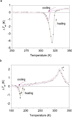
Figure 16. Temperature dependence of the adiabatic temperature change ▵Tad near austenite–martensite transition in Heusler alloys (a) Ni45Mn37In13Co5, transition temperature is around 320 K and (b) Ni50Mn34In16, transition temperature is around 180 K.  corresponds to the Curie temperature of the austenite;
  and
and  .
.
Download figure:
Standard image High-resolution image6.6. Manganites
Ferromagnetic manganites R1−xMxMnO3 are oxides with the perovskite structure, where R is at least one rare earth element and M belongs to the group including e.g. Ca, Pb, Ba, Na1+, Ag1+ and K1+. As oxide materials, manganites have significant advantage over intermetallic magnetocaloric compounds in terms of excellent chemical stability allowing low cost synthesis and various shaping opportunities (Bahl et al 2012, Turcaud et al 2013). A review of the manganite properties can be found in Phan and Yu (2007).
Most ferromagnetic manganites exhibit a second order transition (Phan and Yu 2007, Zhang et al 2012). An exception is La1−xCaxMnO3 with x between 0.25 and 0.5 that exhibits a first order PM insulator to FM metal transition with the concomitant volume change (table 1, Radaelli et al 1995). Due to the low density compared to the metallic materials, the volumetric entropy change in the manganites is moderate (table 6, Mira et al 2002, Phan et al 2005, Phan and Yu 2007). The large heat capacity (see equation (13)) is responsible for the low adiabatic temperature change; only for the La0.67Ca0.33MnO3 composition ΔTad slightly exceeds 2 K in a field change of 2 T (table 6, Lin et al 2006). Consequently, only a small RCPΔS|ΔTad > 2 K can be obtained (figure 12, Bahl et al 2012).
Table 6. Properties of manganites: the peak temperature of the ΔS curve (Tmax), the gravimetric and volumetric maximum entropy change (ΔSmax) and the maximum adiabatic temperature change ( ) in a field change μ0ΔH = (0 − Hf) T.
| Material | Tmax (K) | Hf (T) | −ΔSmax (kJ m−3 K−1) | −ΔSmax (J kg−1 K−1) |  (K) (K) |
Reference |
|---|---|---|---|---|---|---|
| La0.67Sr0.33MnO3 | 370 | 1 | 9.9 | 1.6 | 1.0 | Rostamnejadi et al (2011) |
| 2 | 16.7 | 2.7 | 1.6 | |||
| 5 | 31.9 | 5.15 | 3.3 | |||
| La0.67(Ca0.95Sr0.05)0.33MnO3 | 275 | 1 | 20.2 | 3.26 | Mira et al (2002), Phan et al (2005) | |
| 5 | 65.1 | 10.5 | ||||
| La0.67(Ca0.887Sr0.113)0.33Mn1.05O3 | 275 | 1 | 22.9 | 3.7 | 1.3 | Bahl et al (2012) |
| La0.67Ca0.33MnO3 | 268 | 1 | 1.3 | Lin et al (2006) | ||
| 2 | 42.8 | 6.9 | 2.4 |
6.7. Amorphous and nanocrystalline alloys
Soft magnetic Fe-based amorphous and nanocrystalline alloys as well as rare-earth-based bulk metallic glasses show the conventional second order PM to FM transition with the Curie temperature adjustable in the range of 100–600 K (Maeda et al 1983, Franco et al 2006b, 2012, Gorsse et al 2008, 2011, Ipus et al 2009). A recent review on the MCE in these materials can be found in Franco et al (2012). Favourable characteristics of the Fe-based alloys are good mechanical stability, low cost and chemical resistance. Common to this material type is, however, low absolute value of the entropy change ΔSmax, which is only about half of that observed in Gd (see tables 2 and 7). This is caused by a very wide temperature range (~100 K), where the transition is taking place. The adiabatic temperature change is below 2 K even in a field change of about 2 T (table 7, Law et al 2011). The wide temperature span is often used to calculate the relative cooling power of these materials without taking into account that a sufficient ΔTad is required to move the heat in the regenerator (section 5.1). Since the amorphous and nanocrystalline alloys show  , cooling will not be efficient (figure 12). As discussed in section 5.1, the reduction of the MCE, albeit not so drastic, is also observed in materials with the first and second order transitions, when the grain size is reduced to the nanometer range (Mathew et al 2010, Lyubina 2011).
Table 7. Properties of amorphous alloys: the peak temperature of the ΔS curve (Tmax), the gravimetric and volumetric maximum entropy change (ΔSmax) and the maximum adiabatic temperature change ( ) in a field change μ0ΔH = (0 − Hf) T.
| Material | Tmax (K) | Hf (T) | −ΔSmax (kJ m−3 K−1) | −ΔSmax (J kg−1 K−1) |  (K) (K) |
Reference |
|---|---|---|---|---|---|---|
| Fe90Zr10 | 230 | 1.4 | 9.5 | 1.4 | Maeda et al (1983) | |
| 5 | 27 | 4.0 | ||||
| Fe84Nb7B9 | 299 | 1.5 | 9.8 | 1.44 | Min et al (2007) | |
| Fe75B12Cr8Ce5 | 295 | 1.8 | 1.1 | 1.4 | Law et al (2011) | |
| Fe79B12Cr8La1 | 348 | 1.8 | 1.1 | 1.3 | Law et al (2011) |
6.8. Compounds with order–order transitions
Order–order transitions occur between magnetically ordered states and are distinct from the order–disorder transitions, such as FM → PM transition. The order–order transitions can be subdivided into (i) transitions involving the change in the orientation of the sublattice moments, e.g. transitions between ferromagnetic and antiferro- or ferrimagnetic states, and (ii) transitions, where orientation of the moments is altered only in respect to the crystallographic axes, i.e. spin reorientation transitions (SRT).
Fe–Rh alloys (space group  ) exhibit a strong first-order transition from the FM to antiferromagnetic (AF) state at 320–350 K (figure 9, Shirane et al 1963, Kouvel and Hartelius 1962). Fe49Rh51 was the alloy, where the first experimental observation of the giant MCE was made (Nikitin et al 1990). The MCE in the Fe–Rh alloys is of the inverse type, since the high-temperature phase in these materials is FM and the low-temperature phase is AF with zero net magnetisation. Consequently, on cooling or field application Fe–Rh shows a negative adiabatic temperature change of about
  (µ0ΔH ≈ 2 T) and positive entropy change of about 120 kJ m−3 K for µ0ΔH > 1 T (table 8, Stern-Taulats et al 2014). A large volume change is observed at the transition (table 1). The thermal hysteresis and the rate
  can differ to a great extent depending on the alloy microstructure: between 7.5 K and 50 K and
  and
and  , respectively (Nikitin et al 1990, Manekar and Roy 2008, Chirkova et al 2015). In the most favourable case, the parameters yield
  . As a result of the large hysteresis, the MCE on the second and subsequent cycles is lower compared to the first cycle (Manekar and Roy 2008, Chirkova et al 2015). The considerable hysteresis and high cost of rhodium are disadvantageous characteristics for heat pumping.
Table 8. Properties of materials with order–order transitions: the peak temperature of the ΔS curve (Tmax), the maximum entropy change (ΔSmax) and the maximum adiabatic temperature change ( ) in a field change μ0ΔH = (0 − Hf) T.
| Material | Tmax (K) | Hf (T) | −ΔSmax (kJ m−3 K−1) | −ΔSmax (J kg−1 K−1) |  (K) (K) |
Reference |
|---|---|---|---|---|---|---|
| FeRh | 313–320 | 1 | −123.2 | −12.5 | ≈−5.6 | Nikitin et al (1990), Annaorazov et al (1996) and Stern-Taulats et al (2014) |
| 2 | −123.2 | −12.5 | ≈−13 | |||
| 5 | −123.2 | −12.5 | ||||
| Er2Fe14B (H||c-axis) | 323 | 0.5; 1; 2; 5 | −6.6 | −0.7 | −0.5 | Pique et al (1996), Skokov et al (2009), Basso et al (2011) |
| NdCo5 (rotation from c- to a-axis) | 280 | 1.3 |
15.9 | 1.9 | 1.6 | Nikitin et al 2010 |
At SRT, rotation of the magnetisation induces a change in the anisotropy part of the free energy  with the corresponding change in the entropy term
  . In a uniaxial crystal, the adiabatic temperature change can be written as (Vonsovsky 1971)
where K1 is the uniaxial anisotropy constant and  and
and  is the angle between the magnetisation and the c-axis in the initial and final fields, respectively. Different to the operation of the conventional AMR (section 2), the adiabatic temperature change can be realised by rotation of the magnetic refrigerant in a constant magnetic field or by rotation of the field vector H while keeping the refrigerant stationary.
From the form of equation (18) it is apparent that the MCE is large, when the derivative  is large, which ultimately requires materials with a high magnetocrystalline anisotropy and a SRT of the first order type. The condition is fulfilled e.g. in the R2Fe14B (R = Er, Tm) compounds (space group
  ) showing SRT between the 'easy axis' (
 c-axis) and the 'easy plane' (
 c-axis) (Pique et al 1996). In a single crystal Er2Fe14B,
  saturates at a value of 0.5 K in µ0H = 0.5 T and
  at 6.6 kJ m−3 K in µ0H ~ 0.01 T; in fields above this value the entropy peak broadens (table 8, Skokov et al 2009, Basso et al 2011). A light-rare earth-based compound, NdCo5, also shows a first order SRT from 'easy axis' to 'easy cone' at 280 K (figure 9, Nikitin et al 2010). Larger MCE can be obtained by rotating this refrigerant in 1.3 T compared to R2Fe14B (table 8). However,
  yields negligible relative cooling capacity RCPΔS|ΔTad > 2 K.
6.9. Magnetocaloric effect in films and multilayers
Magnetocaloric effect in thin films is less of application interest, but is mainly interesting from the point of view of understanding the basic phenomena and exploring the ways to improve the performance or even radically change the way the magnetocaloric materials are applied. One of the first publications reporting the MCE in the film form are due to Babkin and Urinov (1989), who studied ΔTad on rotation (see equation (18)) of single-crystal Ni and Fe2O3 films, and Morelli et al (1996), who reported the MCE in 2.4 µm thick La0.67M0.33MnO3 films (M = Ca, Ba, Sr) on LaAlO3 substrates in the vicinity of the magnetic phase transition coinciding with the metal–insulator transition. The entropy change in the manganite films is significantly below that in bulk counterparts, compare ΔS = 0.5 J kg−1 K−1 ≈ 3.1 kJ m−3 K−1 for a field change of 0–1 T in films (Morelli et al 1996) to ΔS values in table 6. Suppression of the ΔS peak height with the concomitant smearing out of the ΔS peak width is also observed in 1–3 µm thick Gd films (Mansanares et al 2013), Gd/W multilayers on MgO substrate (Miller et al 2010) and Gd5(Si,Ge)4 thin films (Hadimani et al 2015). The reduction can be attributed to the finite size scaling effects in nanostructures that has also been observed in bulk systems (Mathew et al 2010, Lyubina 2011) and discussed in section 5.1.
Mukherjee et al (2009) proposed a concept of AF interlayer coupling of the FM layers that would potentially allow one to tailor a metamagnetic transition with a prominent magnetisation discontinuity at the transition. Experimentally observed values of the MCE in a model Co/Cr multilayer system are rather low. Nevertheless, the concept of artificial structures may provide a pathway for the discovery of new materials.
The entropy change in epitaxial 200 nm thick films of La0.8Ca0.2MnO3 on LaAlO3 substrate and La0.7Sr0.3MnO3/SrRuO3 superlattices is of the same value or even exceeds ΔS observed in bulk counterparts (Zhang et al 2011, Debnath et al 2013). The observed ΔS in epitaxial films exhibits an anisotropy with the values of about 36 kJ m−3 K−1 in the ab plane and 25 kJ m−3 K−1 along the c-axis for a field change of 1 T. Debnath et al (2013) attributed the anisotropy in the MCE to a stronger exchange interaction in the manganite intralayer compared to that in the interlayer, forcing the magnetic moments to lie in the ab plane.
A further effect that can play a role in thin film systems is the strain induced in the magnetocaloric film by a substrate. The effect of epitaxial strain induced by various substrates allowing to vary the size and direction (compressive/tensile) of the imposed stress was studied by Kumar et al (2013) in La0.67Sr0.33MnO3 films and by Maat et al (2005) in FeRh films. Moya et al (2013) exploited a first-order structural phase transition in BaTiO3 substrates to create giant and reversible magnetocaloric effects in epitaxial films of La0.7Sr0.3MnO3 via the entropic interconversion of ferromagnetic and paramagnetic phases.
A step further in the direction of manipulating the MCE by stimuli other than the magnetic field was demonstrated by Binek and Burobina (2013). In their theoretical concept, the entropy change in two-phase films consisting of the magnetocaloric material La0.7Sr0.3MnO3 and piezoelectric PbMg0.33Nb0.67O3–PbTiO3 (PMN–PT) is induced by voltage. Various possible geometries (figure 17) were suggested and isothermal voltage-controlled entropy change ~1 J kg−1 K−1 was predicted. Although the effect of voltage on the MCE still needs to be demonstrated experimentally, a step towards experimental realisation of magnetocaloric/piezoelectric heterostructures was devised by the successful growth of epitaxial Heusler-type Ni–Mn–Ga–Co films on PMN–PT substrates (Schleicher et al 2015).
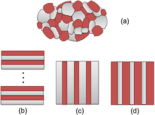
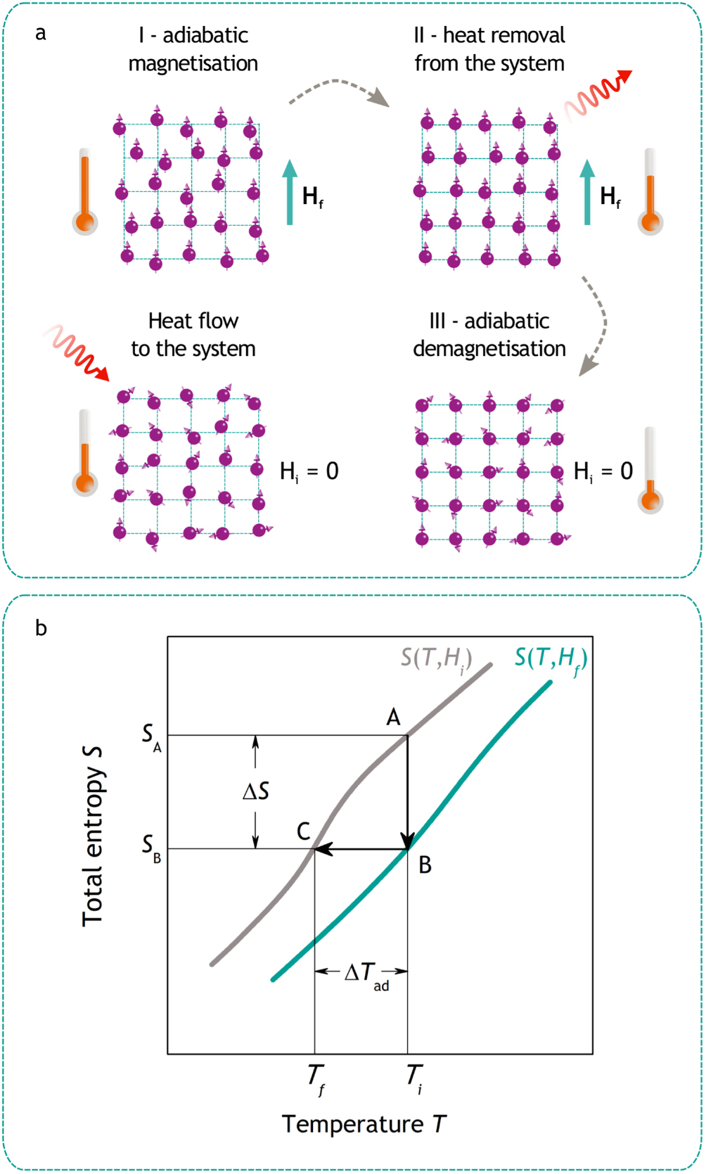
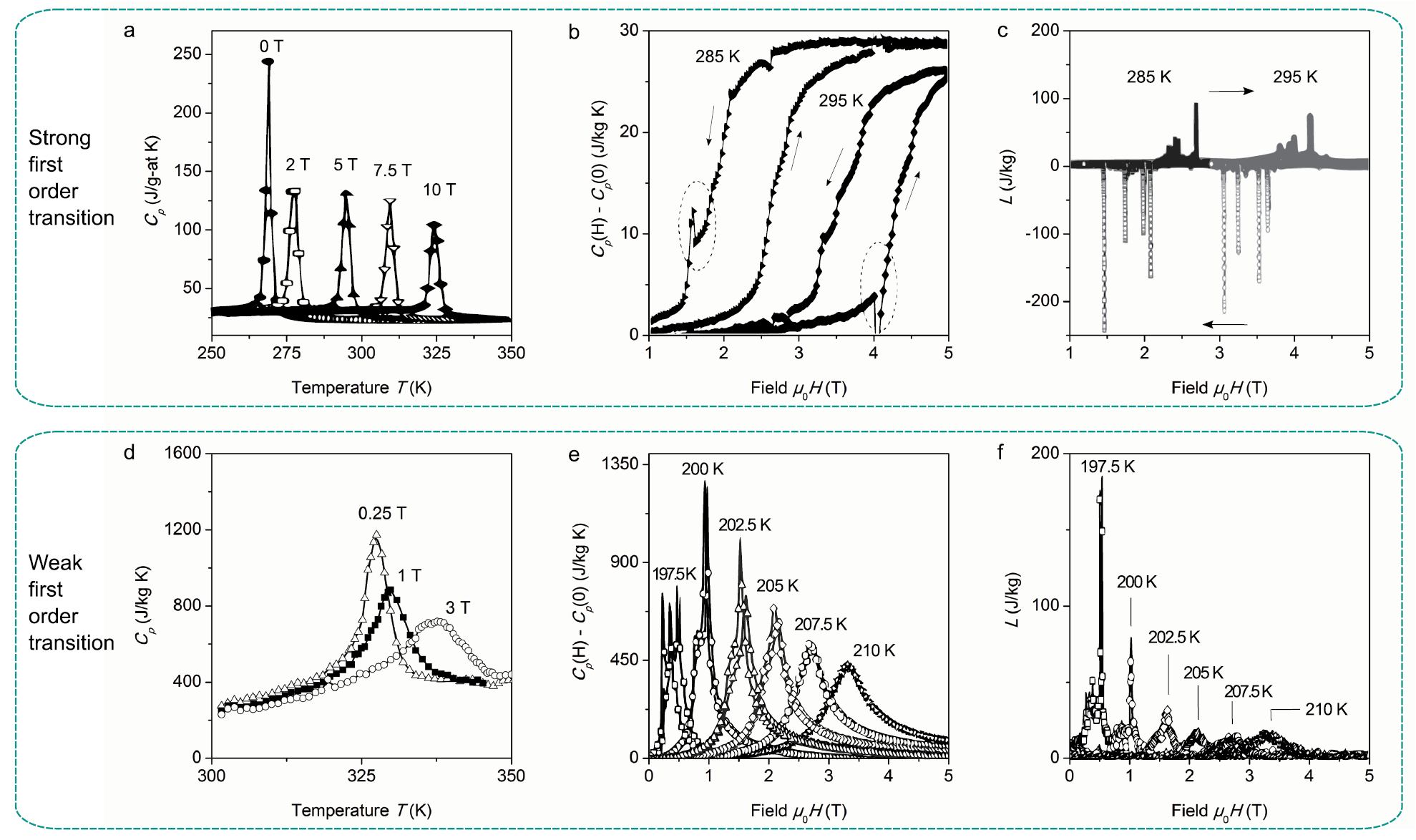
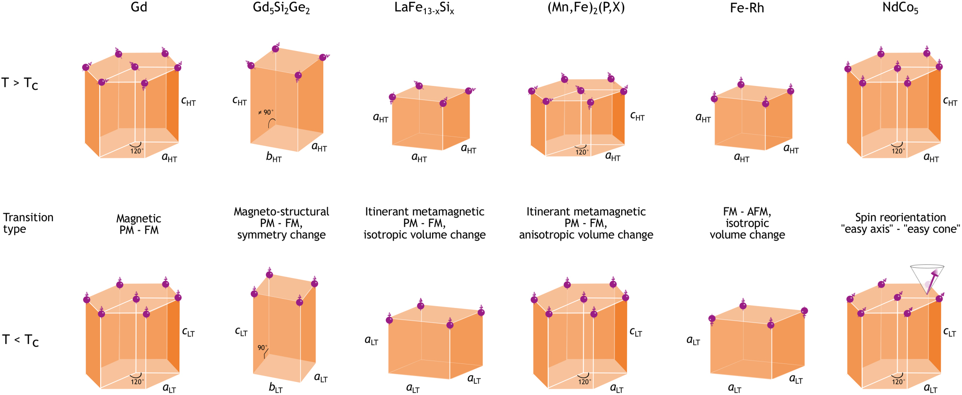
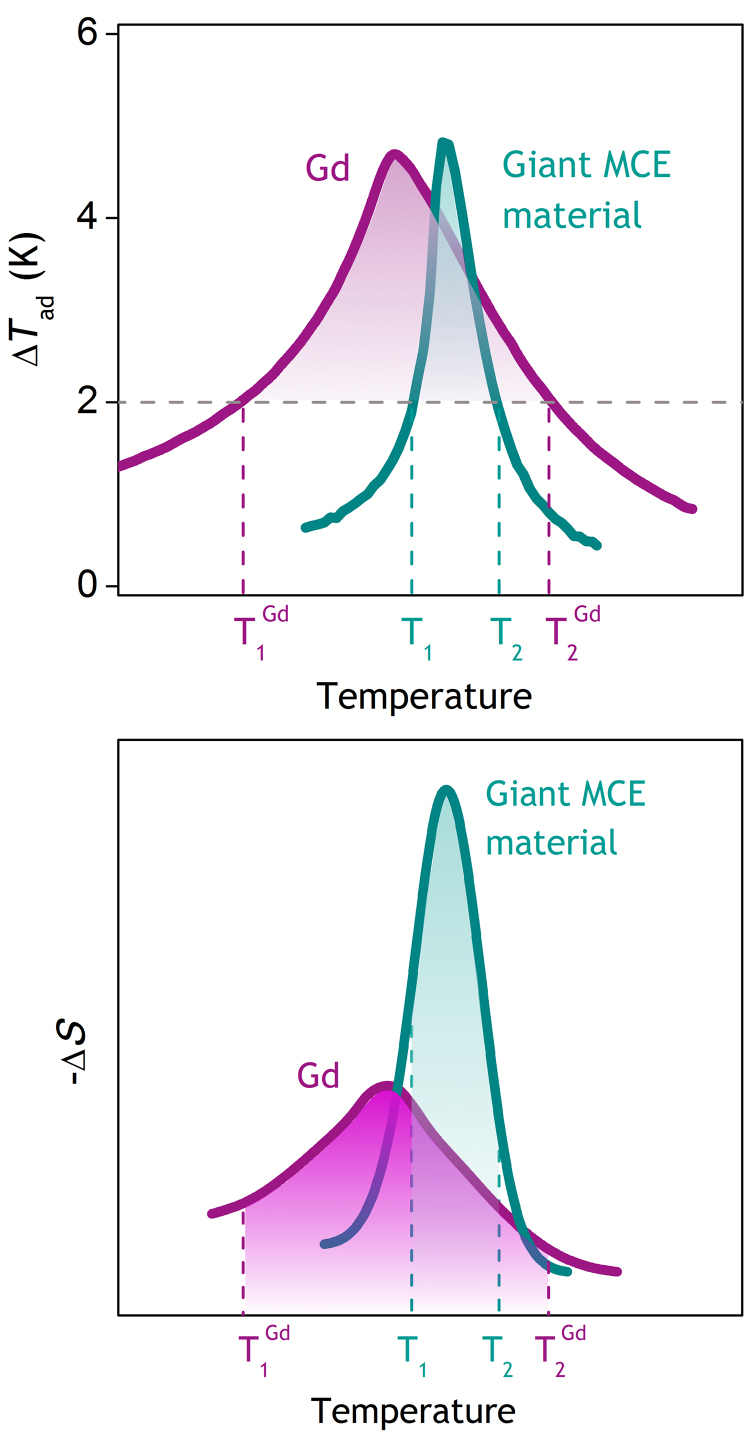
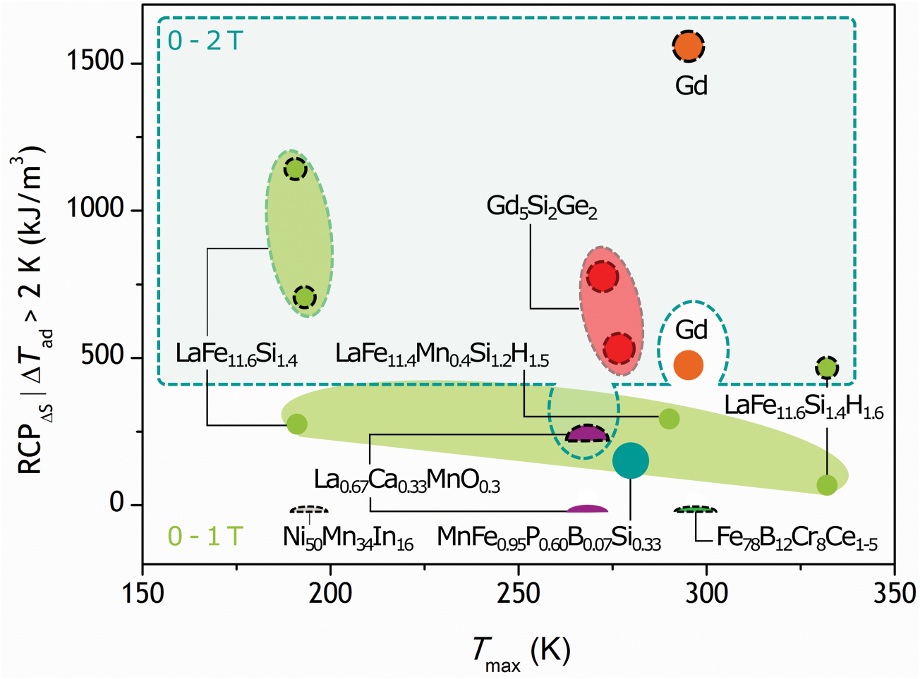
Figure 17. Possible nanofabrication of magnetocaloric materials for voltage controlled entropy change. Magnetic material (light gray) with magnetoeleastic properties such as (La,Sr)MnO3 interacts with piezoelectric material (dark gray/on-line red) such as PMN–PT when brought in close proximity. Possible nanostructured two-phase multiferroics can have grain structure (a), layered heterostructures (b), columnar structure of piezoelectric material in magnetic matrix (c), or vice versa (d) (reproduced with permission from Binek and Burobina (2013). Copyright 2013 AIP Publishing LLC.).
Download figure:
Standard image High-resolution image
Mechanical control of the magnetic properties in thin films with a large magnetostriction offers an interesting route to employ the interaction of surface acoustic waves (SAW) with magnetic excitations to trigger MCE in materials with first order transition. Duquesne et al (2012) demonstrated large ultrasound attenuation in thin epitaxial MnAs films on GaAs that can be ascribed to the strain-induced triggering of the giant MCE in MnAs. The observed effect opens up a new way to control the magnetocaloric effect.
7. Conclusion
In this review, material choices have been analysed in terms of their thermodynamics and applicability for magnetic heat pumping. The analysis indicates that only materials with the giant magnetocaloric effect due to the weak first order transition can find application. These materials have characteristic free energy barriers between magnetic states comparable to the thermal energy,  . The energy barrier is proportional to the magnetic hysteresis,
  ; table 1 shows that the low hysteresis is achieved in some candidate materials, such as LaFe13−xSix and MnFeSixP1−x compounds. Practically, the entropy change in these materials follows the relation in equation (8) and the transition type changes gradually from weak first order to second order on changing the chemical composition. Further reduction of the detrimental hysteresis requires a clear strategy towards appropriate microstructure design, which requires the understanding of the fundamentals of the magnetic phase transitions.
As concerns materials with the strong first order transition, such as Gd5Si2Ge2-based and Ni2MnZ-based Heusler alloys, there is little hope of developing such materials into competitive refrigerants. The considerable hysteresis observed in these materials (table 1) requires magnetic fields  to perform a cooling cycle, which cannot be a practical solution.
The importance of taking into account the adiabatic temperature change ΔTad of the refrigerant materials was emphasised and a relative cooling power parameter, RCPΔS|ΔTad > 2 K, was introduced, defined as an area of the entropy peak limited to the temperature range where ΔTad is above 2 K. Clearly, only materials with the considerably large RCPΔS|ΔTad > 2 K can be deemed as appropriate for applications, whereas the materials where this parameter is close to zero cannot be good refrigerants (figure 12).
Although it cannot be excluded that new magnetocaloric materials will be discovered in the future, the magnetocaloric effect will remain on a similar level as it is today. The fundamental limitation arises due to the fact that the material's relative cooling power is proportional to the magnetisation jump at the transition and is bounded by the product of the saturation magnetisation and the maximum available field,  (Bennett et al 1992, Zverev et al 2010). As we are fundamentally limited in terms of increasing
  , along with negligibly small hysteresis, our quest is to make the MCE as large as possible in as low as possible magnetic field (<1 T).
Significant improvements are equally needed on the side of the magnetic cooling systems. Also in this respect material physicists can make a contribution by developing methods for efficient refrigerant shaping as well as improving thermal management and mechanical and chemical stability of the magnetic refrigerants. In order for the magnetic cooling technology to become economically successful, a coordinated interdisciplinary effort is required.
Acknowledgment
I am grateful for the support that was given to me over several years at the IFW Dresden, Imperial College London, where the data included in this review was obtained, and Evonik Industries AG. I would like to thank all the colleagues at these places who helped and supported me. I am extremely thankful to LF Cohen for the help over the years and U Hannemann for fruitful discussions and proofreading of the manuscript.