


Abstract
Infrared thermography is widely used in non-destructive testing and in the non-destructive evaluation of subsurface defects in several materials. The detection and reconstruction (location and shape) of a defect inside a material from thermal data requires the solution of an inverse heat conduction problem. Here the problem is tackled by the thin-plate approximation of the investigated domain. A number of physical quantities must be known for the reconstruction procedure to be successful: some relating to the material (thermal conductivity, heat capacity, density), usually known, and others relating to the heating process. This paper proposes procedures for accurately measuring the latter, whose importance is often not given due consideration. Those procedures allow us to accurately measure the heat flux distribution produced by the sources on the heated surface, and the heat exchange coefficient at the remaining surfaces, and are easily applicable in 'on field' situations.
Export citation and abstract BibTeX RIS
1. Introduction
Thermography is a non contact and non-destructive technique well suited for the fast detection of subsurface damages in heat conducting structures. Surface temperature maps uk ( ), taken at discrete time instants by means of an infrared camera, are used to verify the integrity of the underlying object. The position, size and shape of the damage can also be identified.
Applications of thermographic nondestructive evaluation have been reported, for example, in the diagnostics of aircraft structures [2, 3], in the integrity analysis of pipelines [4], in the detection of cracks in steel bridges [5] and, in general, in the investigation of thick metallic structures [6, 7]. Thermography is also valuable for the diagnostics and monitoring of poorly conducting materials, like concrete, bricks and, in general, all kinds of masonry [8, 9]. A comprehensive list of the practical applications of thermography can be found in [10]. Interest in the measurement of cracks and defects in materials is continuously increasing, as testified by recent papers dealing with thermographic detection [19, 20, 21] and other measurement methods [22].
In this paper we assume that the specimen is a plate whose top surface is inaccessible to direct inspection and subject to the action of an aggressive environment. The damaged top side is a perturbed planar surface. On the other hand, we can stimulate the object from the bottom side by means of a controlled heat flux ϕ (active thermography). The same side is accessible to infrared vision.
Our approach to the detection and evaluation of inaccessible damage [12, 16] requires a thorough knowledge of both the 'internal' parameters of the problem—the specific heat capacity c, the density ρ and the thermal conductivity κ—and of the 'external' parameters relating to the measurement procedure and to the environmental conditions: the temperature maps uk, the imposed heat flux ϕ, the heat exchange coefficient h, and the initial and ambient temperature U0.
We assume that c, ρ, κ and U0 are known a priori and that the temperature maps uk are given with an error related to the accuracy of the camera. On the other hand, the heat flux ϕ, although related to the technical characteristics of the source and its positioning, remains essentially unknown. The same is true for h whose numerical value is strongly influenced by the environmental conditions close to the inaccessible side of the specimen.
A precise evaluation of ϕ and h is the main goal of the present paper. The importance of the knowledge of such parameters is often underestimated. As an example concerning the characterization of defects by pulsed thermography, although the surface temperature is shown to explicitly depend on the pulse energy ϕ [17], the solution is made independent of ϕ by computing the temperature contrast as the difference between that of the defective area and of a sound neighboring region. Apart from the difficulty of defining a non-defective region (where is it?), that choice implicitly assumes a constant ϕ, a condition usually not met in the real world. Such a difficulty has been highlighted in [18], where the necessity of exactly determining uneven heating is clearly addressed. The adopted 'substitution' technique, however, although valuable in a laboratory framework, is not applicable in real-world situations where a free-sample made having the characteristics of the material under investigation is barely feasible. Similar considerations can be made regarding the heat transfer coefficient h, whose importance is ofter undervalued.
Starting from the observation that ϕ is independent of the specimen, the heat flux is determined using two completely different methods (Fourier one-dimensional (1D) approximation and energy penetration depth) that validate each other, making our solution more robust (section 2). The heat transfer coefficient h is calculated by means of a simplified form of the thin plate approximation (see section 4 and [12]).
1.1. The experimental framework
A number of sources, usually lamps, heat the specimen from the accessible side. The other sides of the plate are subjected to natural or forced convection. The defect to be detected is located on the opposite inaccessible surface. Temperature maps are acquired by means of a thermographic camera.
Figure 1 shows the laboratory setup. Two high-power spotlights (1 kW each) are placed and focalized so as to produce a high heat flux density on the central region of the plate. The flux, as we will see in the following, has a parabolic shape. A thermographic image is acquired before the heating and for some hundreds of seconds after power on, at intervals of 5–6 s, by means of an FLIR B335 thermal camera.

Figure 1. A typical measurement setup for active thermography.
Download figure:
Standard image High-resolution image1.2. Details of the mathematical model
In mathematical terms, evaluating the damage means solving an inverse problem of the class of inverse heat conduction problems (see, for example, [1]).
Observe that our plate-shaped structure has one dimension (thickness) significantly smaller than the other two. More precisely, let  represent the undamaged plate:
  (
( ). Let
  be the volumetric heat capacity. The specimen is assumed homogeneous and isotropic so that c, ρ and κ are positive scalar constants. We refer to [11] for a complete background regarding the classical theory of heat.
The accessible surface ![$S_B=\{(x, y, 0) x, y \in [-\frac{L}{2}, \frac{L}{2}] \}$](https://content.cld.iop.org/journals/0957-0233/28/10/105403/revision2/mstaa7ce1ieqn006.gif) is heated by means of a device (e.g. the lamps) producing a heat flux
is heated by means of a device (e.g. the lamps) producing a heat flux  , constant in time, through SB.
The damaged specimen, that we denote by  , consists of a 'deformed' version of
  in which the top inaccessible surface
 ![$S_{T}=\{(x, y, a) x, y \in [-\frac{L}{2}, \frac{L}{2}] \}$](https://content.cld.iop.org/journals/0957-0233/28/10/105403/revision2/mstaa7ce1ieqn010.gif) changes into
changes into ![$S_\epsilon=\{(x, y, a-\epsilon \theta(x, y)) x, y \in [-\frac{L}{2}, \frac{L}{2}] \}$](https://content.cld.iop.org/journals/0957-0233/28/10/105403/revision2/mstaa7ce1ieqn011.gif) , where
, where  is a scale factor of the 'shape' function
  that describes the deviation from a planar surface.
The temperature maps of the bottom side of  are
are  for
for  . When we begin to collect the temperature maps, the temperature is U0, which is also the external environmental temperature.
Detecting the damage requires us to solve the following inverse problem IP:
Identify the function  from the knowledge of
- 1.The thermal contrast
 for .
for . - 2.The flux ϕ and the heat exchange coefficient h.
- 3.The physical parameters U0, ρ, c and κ.


Actually, assuming that the physical parameters are known, the only available data consist of the sequence of the temperature maps  .
.
In this paper we show how to determine reliable approximated values of ϕ, h and, consequently,  . We do this by exploiting typical features of stepped heating thermography (see [10], section 9.3). Once ϕ and h are known, it is easy to compute the background temperature of
  .
.
This inverse problem is framed in the following initial boundary value problem (IBVP) for the heat equation:

in
with boundary conditions (called Robin or third kind) that account for energy exchanges between the specimen and the environment:

where  and initial data

Here, un is the outward normal derivative (normal with respect to the boundary  ) and
) and  is the diffusivity. The heat exchange coefficient h is related to the geometry of the specimen and to the environmental conditions close to
  . We assume
  is constant at
  ;
;  on the vertical sides of the plate. As for the heat flux, we assume that ϕ is concentrated on SB (i.e.
  for
for  ). As long as ϕ is constant in time we say that we are dealing with stepped heating thermography. Finally, we suppose that U0 is the same on SB and on ST or
  and that the initial temperature is
  .
.
The direct IBVP (1)–(3) is well posed, whilst the inverse problem IP is not. It means, in practice, that a given temperature distribution on the surface SB is 'compatible' with several shapes and scale parameters. A solution of the inverse problem can be obtained by a semi-explicit formula [12] or applying a suitable regularization strategy to treat ill-posedness using genetic algorithms, artificial neural networks, or other techniques to minimize an appropriate cost function ([7, 13, 14, 15] to cite only a few examples).
2. Evaluation of the heat flux
An easier approach to the 'on field' determination of heat flux consists of using a thermally insulating screen, for example, a plywood white-painted panel. That screen is placed in front of the surface of interest so as to receive exactly the same energy density. If the flux density  is constant in space and time, the temperature
  is independent of x and y. Indeed, it can be computed as a series dependent on z and t [11]:
where  ,
,  are the real roots of
  and
and  .
.
As the nth root  belongs to the interval
 ![$[(n-1)\pi, (2n-1)\pi/2]$](https://content.cld.iop.org/journals/0957-0233/28/10/105403/revision2/mstaa7ce1ieqn040.gif) , a short time (a few seconds) yields very large exponents in (4) for
, a short time (a few seconds) yields very large exponents in (4) for  , for the assumed values of the physical and geometrical parameters α, κ, h and a. Therefore, the first term of the series (4) provides a sufficiently good approximation of the background temperature.
For low values of κ (negligible longitudinal heat transfer) and t (negligible dependence on h before a time  ), equation (4) can be used successfully for recovering ϕ from u0. It gives us complete quantitative information about the heat flux. It comes from formula (4) that a constant flux
  is determined by one temperature measurement taken in the first few seconds.
Assume that ϕ is a generic smooth positive function so that it can be approximated by the trigonometric polynomial
The coefficients  for
for  can be recovered from the knowledge of the temperature
  measured on the accessible surface
  at suitable times.
Let  be the solution of the following two-dimensional (2D) IBVP:


We observe that the solution of the 1D problem (4) for a given constant ϕ allows us to closely estimate the solution in  of the above 2D problem for times sufficient to give a small 'Fourier number', i.e.
  .
.
There is numerical evidence that for an arbitrary heat flux described by (5), an approximated solution could be obtained by superposition:
with
for  , where λ, the
  s and
s and
(a finite truncation of the series appearing in the analytical solution of the unidimensional problem (4)).
For a plywood panel with a thickness of 10 mm, the Fourier number is lower than 0.2 for times up to about 200 s. In such conditions, for any N:

Since we know  from our thermal measurements, we can compute the ujs by means of the scalar products
Finally, we invert relations (7) and determine the  s. In particular, we get
We observe that the 'theoretical'  s are time-independent although they are infinite sums of the time-dependent quantities
  and
and  . We expect that the numerical approximations produced here are slightly dependent on
  as a consequence of both the truncation of the series and the noise/uncertainty on the temperature data.
An alternative way to compute the heat flux would therefore be appreciated as a validation tool. A simple estimate of ϕ can be obtained by measuring the temperature behavior on a thermal insulating plate subjected to the same heat flux density ϕ. As before, over short timescales the low thermal conductivity allows us to consider the problem as unidimensional because the lateral diffusion is negligible and the heating of the plate is nearly adiabatic. The thermal energy  in the specimen, per unit width of the plate, is straightforwardly related to the integral of the temperature at time t over the plate thickness:
and the heat flux is computed from the energies at two close times t1 and t2:
Of course, we cannot measure the temperature profile  inside the plate. The temperature measured on the accessible surface
  ,
,  can be used to determine a depth δ at which
  . It can be easily demonstrated that such a depth is related to the so-called thermal penetration depth:
The above derivation is rigorously true when ϕ is constant, independent of x. At times t1 and t2 such that  , the heat flux is given by:
the last square root term being the effusivity of the insulating plate. The formula (13) can also be used in the case of a variable flux,  , at timescales short enough to neglect the heat diffusion. Figure 2 compares the ϕ obtained from the series (5) with
  with the approximation (13) for a true heat flux
  . Temperature data have been obtained on a simulated wooden plate of width
  m and thickness
  mm, having thermal parameters
  ,
,  kg
kg  ,
,  , and assuming
  on the top surface of the plate.
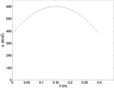
Figure 2. Comparison between ϕ reconstructed by Fourier analysis (solid line) and the short-time approximation (circles).
Download figure:
Standard image High-resolution imageIn section 5 we will see how the above procedure is applied on real thermographic data.
3. Heat exchange measurement
The heat exchange coefficient h can be measured by means of the 'lumped-capacitance' method [23], briefly summarized in the following. An homogenous object of volume V and external surface  is initially at temperature Ui. From time
  the object exchanges energy with the environment at temperature Ua. The heat balance equation for that system

is formally identical to the discharge equation for an electrical capacitor, and has the following solution:

with the time constant τ given by
If the volume is a parallelepiped of the base surface L2 and height  ,
,  .
.
Experimentally, a small aluminum sheet (size  mm) is heated by a heating plate up to a temperature of about 80 °C, with an ambient temperature of 21.9 °C. The temperature decay, measured by means of a thermocouple inserted in a small hole in the lateral surface, is recorded up to equilibrium conditions. Fitting an exponential to figure 3 and solving (16) for h, we obtain
  .
.

Figure 3. Temperature decay in the lumped-capacitance experiment.
Download figure:
Standard image High-resolution image4. Recovering h and ϕ from thermal data by means of thin plate approximation
When the object under investigation is a metal sheet, e.g. an aluminum plate, the external parameters can be obtained simultaneously during the thermographic measurement. In that case none of the procedures outlined in section 2 can be applied because the Fourier number is too small. Instead, we can apply the thin-plate approximation (TPA) to the non-defective domain  of the specimen to obtain an expansion of ϕ and h in powers of the plate thickness a. In the 2D approximation,
  represents a
  plane 'far' from the defect.
The temperature of  for
for ![$t \in (0, T_{\rm max}]$](https://content.cld.iop.org/journals/0957-0233/28/10/105403/revision2/mstaa7ce1ieqn087.gif) , fulfills the heat equation
, fulfills the heat equation

with boundary conditions

and initial data

As usual we scale the thickness variable:  . We have also scaled the heat flux
  and the heat transfer coefficient
  because in this way we get an expansion in even powers only. More precisely, the IBVP becomes
with boundary conditions


and initial data

Since v0 is independent of ζ, if we take the temperature maps at two instants  , we have the linear system


whose solution comes from a straightforward calculation:
and

once the physical parameters κ, ρ and c, typical of the material at hand, are known.
The desired values of ϕ and h are computed by an iterative procedure, computing an initial value of h by means of (24) and alternatively applying equation (25) to the computation of ϕ and h until convergence is reached in both parameters. A simulation run on a 2D aluminum plate covered with a high-emissivity material (as in the experimental conditions) on the bottom surface, subjected to a 'cylindrical' heat flux identical to that plotted in figure 2, and exchanging heat at a rate  at the top surface (the reason the value is so 'high' will be clear in the following), allows us to test the iterative procedure. Figures 4 and 5 show the convergence of
  (the maximum of ϕ) and h, to values nearly identical to the true ones:
  ,
,  .
.
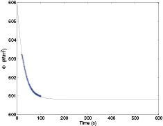
Figure 4. Convergence of the heat flux ϕ.
Download figure:
Standard image High-resolution image
Figure 5. Convergence of the heat exchange coefficient ϕ.
Download figure:
Standard image High-resolution imageFigure 6 shows the heat flux error dependence on the X coordinate: the comparison with that obtained on a thermally-insulating panel (see figure 2) is very satisfying, confirming the reliability of the procedure.
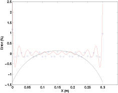
Figure 6. Relative error of the heat flux computed by the TPA-based iterative procedure (black line), compared to those computed by the Fourier method (red line) and by the short-time approximation (dots) on the wooden panel.
Download figure:
Standard image High-resolution image5. Experimental results
The computation based on the TPA assumes a 2D geometric domain. That essentially means that the true heat flux ϕ, having an almost parabolic shape in both coordinates x and y, is assumed to have a cylindrical shape (uniform along y). This, in turn, means that no heat dispersion is assumed along y. Therefore the h value is over-estimated by the above procedure because all heat is assumed to escape from the line  . We call heff such an 'effective' h-value. A comparison among a 3D realistic model of the plate under measurement and the 2D model used in the TPA allows us to obtain the relation between h and heff. Figure 7 shows that such a relation is linear, the slope of the straight line only depending on
  .
.
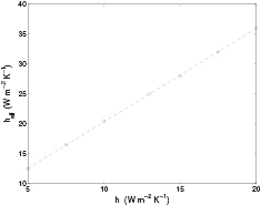
Figure 7. Relationship among heff and h.
Download figure:
Standard image High-resolution imageThe linear relationship shown in figure 7 completes the procedure described in section 4:
- The iterative computation gives and heff.
- A similar procedure can be applied to obtain , or this last can be estimated by a simple proportion between the X and Y dependence of the temperature.
- Once is known, the linear relation among the true (unknown) heat exchange h and heff is obtained by a numerical simulation, allowing us to obtain the correct h.


Two problems arise when trying to heat a bare metallic surface [12]:
- (i)The very low emissivity (e.g. lower than 0.1 for a polished aluminum surface) prevents the material from being significantly heated.
- (ii)The high reflectivity makes it impossible to take thermographic images of the heated surface because any object (including the heating lamps) is reflected into the thermographic camera.
The above well-known problems [10] are usually solved by covering the surface with a high-emissivity paint. Such an approach, while suitable in the laboratory, appears to be rather unpractical and usually too invasive for a real wall. Looking at the published emissivity tables of common materials (e.g. [10], table 8.1), matt paper appears to have an emissivity greater than 0.9. That suggests to us the possibility of using an adhesive paper sheet to overcome the emissivity/reflectivity problem.
Figure 8 schematically shows the geometry of the heated plate.
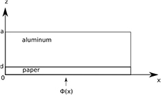
Figure 8. Schematic of the cross section of the metal plate covered by a thin paper sheet.
Download figure:
Standard image High-resolution imageThe influence of the paper sheet on the temperature distribution can be described in terms of its thermal resistance. Actually, in steady-state conditions, the thermal conductivity of the paper-covered plate is obtained by an electric-equivalent circuit as a series of two conductances (paper sheet and aluminum plate, respectively). In transient conditions, the effect of the thermal resistance of the paper sheet can be taken into account by developing the temperature in a Maclaurin series of its thickness d. Thanks to the very small value of d, we can assume the first term as dominant, therefore the temperature of the interface between the paper and the aluminum is given by

kp being the paper conductivity.
Figure 9 shows the experimental heat flux measured on a plywood panel for a given placement of the heating lamps during an experimental session.
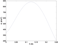
Figure 9. Experimental heat flux.
Download figure:
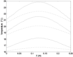
Standard image High-resolution imageAfter replacing the plywood panel with the aluminum plate, equation (26) allows us to compute the temperature on the paper/aluminum interface from the thermographic images taken during heating. Figure 10 shows the effect of the correction for the paper thermal resistance at three time values.
Figure 10. Measured surface temperature (solid line) and temperature computed at the paper/aluminum interface (dashed line), after 60, 180 and 300 s heating time.
Download figure:
Standard image High-resolution image
The effective heat exchange coefficient is computed from the corrected temperature maps according to the procedure outlined in the previous section. The value obtained is  , corresponding to a true
 , in good agreement with that obtained by the lumped method in section 3.
6. Conclusions
Knowledge of the heat flux and the heat exchange coefficient is mandatory for a correct application of active thermography to the non-destructive testing of 'thin' plate structures. The procedures developed in this paper allow the evaluation of both parameters. The reliability of such procedures has been tested on numerical models simulating the true experimental conditions, and then subsequently applied to an experiment. In particular, an approach based on the thin plate approximation allowed us to obtain an accurate estimate of the heat exchange coefficient (as compared to the values obtained by the lumped-constant method). The same approach also allows us to estimate the heat flux intensity and spatial distribution, although that parameter is accurately and robustly measured by means of a non-conducting panel placed in front of the accessible surface of the metal plate under evaluation.