


Abstract
Cone-beam x-ray computed tomography (XCT) is a radiographic scanning technique that allows the non-destructive dimensional measurement of an object's internal and external features. XCT measurements are influenced by a number of different factors that are poorly understood. This work investigates how non-linear x-ray attenuation caused by beam hardening and scatter influences XCT-based dimensional measurements through the use of simulated data. For the measurement task considered, both scatter and beam hardening are found to influence dimensional measurements when evaluated using the ISO50 surface determination method. On the other hand, only beam hardening is found to influence dimensional measurements when evaluated using an advanced surface determination method. Based on the results presented, recommendations on the use of beam hardening and scatter correction for dimensional XCT are given.
Export citation and abstract BibTeX RIS
1. Introduction
X-ray computed tomography (XCT) is a radiographic scanning technique used to visualise the internal and external structure of an object non-destructively. XCT is well-suited for the dimensional measurement of manufactured parts that have complex internal and external features that would otherwise have to be cut open in order to be measured with a tactile or optical instrument.
With XCT it is possible to measure an object in three-dimensions with micron-level spatial resolution, scan times can be as short as a few minutes and entire assemblies can be measured in a single scan [1, 2]. However, XCT is not without its shortcomings, instabilities in the imaging system may influence measurement results [3] whilst misalignment of the system geometry can cause systematic measurement errors [4]. One prominent source of CT image degradation is the presence of artefacts in the reconstructed data [5]. Artefacts may arise due to non-linearities in x-ray attenuation caused by the physical processes of beam hardening and x-ray scattering; the influence of these two phenomena on dimensional measurements is studied in this work.
If XCT is to be used with confidence for making dimensional measurements then the traceability of measurements must be ensured. A measurement result must be accompanied by a statement of uncertainty if it is to be traceable. The uncertainty of a measurement can be evaluated by propagating the uncertainty due to each factor that influences the measurement result [6]. Presently there is very little understanding on how various influencing factors affect XCT measurements. This work focuses on characterising one influencing factor, namely non-linear x-ray attenuation, that arises due to scatter and beam hardening.
1.1. Scatter and beam hardening
Filtered backprojection (FBP) is an algorithm commonly used for tomographic reconstruction. FBP is used under the assumption that x-ray attenuation is linearly proportional to material thickness [5]. This relationship is described by the Beer–Lambert law of attenuation and is written as follows:

where  is the intensity of the incident x-ray beam,
  is the intensity of the x-ray beam after passing through a material part of thickness
  , and
, and  is the linear attenuation coefficient which is a material property and a function of x-ray energy
  . The Beer–Lambert law of attenuation can be shown experimentally with the apparatus illustrated in figure 1(a). A monochromatic beam of x-rays should be used and the beam should be collimated both before and after passing though the object. For cone-beam XCT quite a different arrangement is used, this is illustrated in figure 1(b). A polychromatic cone-beam of x-rays is used alongside a flat-panel detector. In this arrangement x-rays scattered by the object will raise the total detected signal and reduce the measured attenuation, thus equation (1) may be rewritten [7]

where  is the scatter signal and is a function of x-ray energy and the atomic number of the material
  .
.

Figure 1. Illustration of apparatus for measuring x-ray attenuation. (a) Monochromatic x-ray source and pencil beam geometry, leads to linear x-ray attenuation. (b) Polychromatic x-ray source and cone beam geometry (side view), leads to non-linear x-ray attenuation.
Download figure:
Standard image High-resolution imageIn addition to the presence of scatter, industrial cone-beam CT systems use a polychromatic x-ray source. For polychromatic x-rays the total measured x-ray attenuation is the sum of attenuation for each x-ray energy thus equation (2) is integrated with respect to x-ray energy and rewritten as:
where  and
and  are the minimum and maximum energies of the x-ray spectrum respectively and
  is a function describing the energy dependence of an XCT system, i.e. the x-ray spectrum and the quantum absorption efficiency of the x-ray detector [8].
Polychromatic x-ray attenuation poses a problem similar to scatter since it influences attenuation measurements. When a polychromatic x-ray beam passes through matter, low energy (soft) x-rays are attenuated more easily than high energy (hard) x-rays3. This preferential attenuation of low energy x-rays raises the mean energy of the x-ray beam as it passes through an object, the beam becomes more difficult to further attenuate, i.e. the beam becomes more penetrating and is said to become harder, this effect is called beam hardening. As a result of beam hardening the outer surface of an object will be measured as highly attenuating since this is where most of the low energy x-rays of the incident beam are attenuated. On the other hand the centre of the object will be measured as less attenuating since this is where the x-ray beam is harder and therefore more penetrating, this leads to the well-known cupping artefact [5].
Clearly there is a considerable difference between equations (1) and (4), that is to say, scatter and beam hardening cause the relationship between x-ray attenuation and material thickness to change from a linear relationship, to a non-linear relationship. Given that the FBP reconstruction algorithm assumes the relationship is linear, scatter and beam hardening cause artefacts in the reconstructed data, these artefacts include: false density gradients (cupping), streaks between highly attenuating features and a general loss of contrast. The presence of these artefacts causes problems when evaluating dimensional measurements from CT data-sets. In order to evaluate dimensional measurements from CT data the position of the object's surface must first be identified, this requires 3D edge detection. It has been shown that both scatter and beam hardening artefacts change the shape of edges in CT data, this change in edge shape causes the estimated edge position to move which influences dimensional measurements evaluated from the determined surface [9–11]. Scatter and beam hardening artefacts may be so severe that flat surfaces appear to be curved and thin walls appear to have holes in them [2]. Even when these artefacts are not so severe the extent to which scatter and beam hardening influence dimensional measurements is not well understood. This paper addresses this gap in the knowledge through the use of simulated data.
1.2. Previous work
Scatter and beam hardening are well known to degrade the quality of CT data, thus a large number of methods exist to correct the effects of scatter and beam hardening. The objective of these corrections is to remove cupping and streaking artefacts and to increase image contrast and the signal-to-noise ratio of the data; in many cases these corrections simply aim to make the data look better. When it comes to making traceable dimensional measurements from CT data the underlying influence of scatter and beam hardening on dimensional measurements should first be understood, then the effect of correcting these artefacts should be understood, only then the measurement uncertainty due to these influences can be correctly evaluated.
The influence of scatter and beam hardening on dimensional measurements is acknowledged in the literature [1, 2], however, few dedicated studies on the topic have been published. A number of authors have studied the influence of beam hardening correction on the accuracy of dimensional measurements [9–15]. These studies have shown that a linearization beam hardening correction can be used to reduce measurement errors. However, all these studies neglect the presence of scatter and its contribution to the non-linearity of attenuation values. The objective of this work is to study the influence of both scatter and beam hardening on dimensional measurements evaluated from simulated XCT data.
2. Method
The influence of scatter and beam hardening on dimensional measurements is investigated using simulated data. A simulation-based approach is chosen in order to isolate the influencing factors which is difficult or even impossible to do experimentally. XCT scans of an object are simulated with and without scatter, beam hardening, beam hardening correction and a combination thereof, see table 1. The details of the object, simulation software, simulated scan parameters, beam hardening correction and data processing are described in the sections that follow.
Table 1. Details of the conditions under which the object is simulated. 1 indicates with condition, 0 indicates without condition.
| Run | Scatter | Beam hardening | Beam hardening correction |
|---|---|---|---|
| 1 | 0 | 0 | 0 |
| 2 | 1 | 0 | 0 |
| 3 | 0 | 1 | 0 |
| 4 | 1 | 1 | 0 |
| 5 | 1 | 1 | 1 |
| 6 | 0 | 1 | 1 |
2.1. Object
The size, geometry and material of a scanned object will influence the amount of scatter and beam hardening present in a measurement result. The size of the object influences x-ray path lengths and thus the attenuation suffered by a beam; large objects and dense materials are scanned with higher energy x-rays to ensure sufficient penetration. The geometry of an object influences the complexity of the resulting artefacts, for example, a uniform rod will lead to a simple cupping artefact, whist an object with a complex geometry will lead to a complex combination of cupping and streaking artefacts. The material of an object influences the probability of certain x-ray-matter interactions occurring: materials with high atomic numbers and densities absorb x-rays more easily whereas Compton scatter is strongly dependent of the number of outer shell electrons and the density of a material.
The object considered in this study is the pan flute gauge (PFG) developed by the Laboratory of Industrial and Geometrical Metrology, University of Padova, Italy (see figure 2). The PFG consists of five calibrated borosilicate glass tubes supported by a carbon fibre frame, the five tubes have the same nominal inner and outer diameters but have different lengths, see caption of figure 2 for dimensions. Diameters and lengths of the PFG were calibrated using a tactile coordinate measuring machine [16].
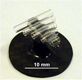
Figure 2. The PFG (five calibrated glass tubes supported by a carbon fibre frame) developed at the University of Padova, Italy. Nominal tube lengths (mm): 12.5, 10, 7.5, 5, 2.5. Nominal inner and outer diameters: 1.5 mm and 1.9 mm respectively.
Download figure:
Standard image High-resolution imageThe PFG is chosen for this study for three reasons: firstly, previous studies characterising the influence of scatter and beam hardening on dimensional measurements have considered metallic objects [10]. XCT is very well suited for measuring lower density materials that can scatter strongly so these types of materials should also be studied. Figure 3 shows the probability of x-rays undergoing photoelectric absorption, Rayleigh and Compton scattering interactions for different x-ray energies for borosilicate glass, at around 50 keV Compton scattering becomes the dominant x-ray interaction, thus the PFG can be expected to generate a significant scatter signal. Secondly, the PFG was used in the CT Audit [16], an international comparison of XCT systems for dimensional metrology, a wealth of experimental data is therefore available for the object. Thirdly, the object is comprised of simple geometric features that present bidirectional dimensions that will be influenced to varying degrees by scatter and beam hardening, these being the inner and outer diameters and the length of each tube.
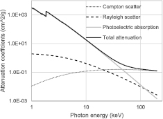
Figure 3. Graph of photon cross sections for Compton and Rayleigh scattering, photoelectric absorption and total attenuation coefficient for borosilicate glass of composition  . Data downloaded from [17].
Download figure:
Standard image High-resolution image2.2. Simulation overview
XCT scans of the PFG are simulated using software developed in-house. The simulation is based on ray-tracing and considers the following physical phenomena: beam hardening, scatter, the x-ray focal spot size and noise. The x-ray focal spot size is considered in the simulation because it is often the factor that limits the spatial resolution of projections and will therefore influence the quality of edges in projections and reconstructed data. The quality of edges in CT data influences surface determination and hence dimensional measurements. Noise is taken into consideration since x-ray images are a result of random x-ray-matter interactions that lead to statistical noise: the noise in a CT data-set will again influence the determined surface and hence dimensional measurement results.
The basic simulation procedure is as follows
- 1.X-ray path lengths
 through the object are calculated for each angular position of the object via ray tracing.
 - 2.Using the ray path lengths, x-ray attenuation is calculated using a look up table generated from measured data.
- 3.Scatter signals are calculated and added to the intensity images.
- 4.Randomly generated noise is added to each projection.

A detailed description of each step of the simulation is described in the sections that follow.
2.3. Ray tracing and beam hardening
Ray tracing is a computer graphics technique for rendering images of 3D scenes. The technique requires the start and end coordinates of a ray be defined alongside a geometric primitive through which the ray passes. Using vector mathematics it is possible to calculate the ray path length through the object. Rays are traced from a circular source to each pixel in a detector array. This is repeated for each angular orientation of the object, hence the output of the ray tracing algorithm is a set of images that describe the x-ray path lengths through the object.
Beam hardening is simulated by converting x-ray path lengths to polychromatic attenuation, the function used for this conversion is derived from measured data. Polychromatic attenuation is measured experimentally for increasing thicknesses of borosilicate glass: 1 mm to 20 mm in 1 mm steps. The resulting relationship between polychromatic attenuation and material thickness is plotted in figure 4. A 6th order polynomial is fitted to the curve giving an R2 value of 1, this polynomial function is used to simulate polychromatic attenuation for a given material thickness. The XCT system settings used for the attenuation measurements are as follows: the source voltage and current are set as 140 keV and 71 µA respectively, the detector exposure time is 1 s with no projection averaging, the source-to-object distance is 65 mm and the source-to-detector distance is 1165 mm, the XCT system used is a Nikon MCT225. These settings are typical for CT measurements of the PFG at the University of Padova.

Figure 4. Attenuation measurements of borosilicate glass, with and without scatter. The polynomial function is used to convert x-ray path lengths through the workpiece to polychromatic attenuation.
Download figure:
Standard image High-resolution imageFrom the discussion in section 1 it can be assumed the attenuation measurements will be contaminated by scattered x-rays. To overcome this a second set of measurements are made with a lead blocker placed between the x-ray source and the borosilicate glass. The lead blocker absorbs all x-rays incident on it such that any signal measured in its shadow must be due to scattered radiation. These scatter signals are subtracted from the unblocked measurements such that the attenuation measurements are not contaminated by scatter. Both attenuation measurements with and without scatter are plotted in figure 4. In section 2.5 the scatter free and scatter contaminated polychromatic attenuation measurements are used to validate the accuracy of the scatter model, which is described in section 2.4.
To simulate monochromatic x-ray attenuation the Beer–Lambert law of attenuation is used, see equation (1). The linear attenuation coefficient  is defined as the gradient of the least-squares line that passes through the origin of the scatter-free attenuation measurements; this gives a value of
  of 0.7 cm−1 which corresponds to an x-ray energy of approximately 50 keV.
2.4. Scatter
Scatter signals  are simulated by convolving primary x-rays
  with an analytically derived scattering point spread function
  [18, 19]. The resulting scatter signal is then added to the primary signal which yields the total detected signal
  :
:

where

The symbol  denotes convolution of
  and
and  . The scattering point spread function (PSF) is derived based on the sum of the angular distributions of Rayleigh and Compton scattering. The Klein–Nishina formula describes the differential cross section for Compton scattering [18]:
Where  is the Compton scattering cross section,
  is the solid angle,
  is the classical electron radius,
  is the photon frequency before a scattering interaction,
  is the photon frequency after a scattering interaction, and
  is the scattering angle. The photon frequency after a scattering interaction can be calculated using the Compton wavelength shift equation but for the x-ray energies considered here the change in photon energy is very small, such that
  [20]. The Klein–Nishina equation is therefore simplified to:
The Klein–Nishina formula is based on the assumption that the electrons of a target atom are initially at rest and free, however, in real atoms the electrons are neither at rest nor free. This discrepancy leads to departures from the Klein–Nishina expression. These departures can be addressed by multiplying the Klein–Nishina formula by the incoherent scattering function  in which
  is the momentum transfer and
  is the atomic number of the scattering atom. Thus the differential cross-section for Compton scattering is written:
where

Hubbell's tabulations of the incoherent scattering function for silicon have been used here since silicon is the main constituent of borosilicate glass [21]. Integrating the differential cross-section for Compton scattering with respect to the scattering angle  gives the desired angular scattering distribution and hence the Compton scattering PSF.
The differential scattering cross section for Rayleigh scattering is:
where  is the atomic form factor. Form factors introduce an energy and material dependence that is not taken into account in the Rayleigh formula. At low photon energies form factors do not affect the angular distribution of Rayleigh scattering but at higher energies they are forward peaked. Again, Hubbell's tabulations are used for the atomic form factors for silicon [22].
Integrating the differential scattering cross section for Rayleigh scattering with respect to the scattering angle  gives the desired angular scattering distribution and hence the Rayleigh scattering PSF. The total scattering PSF is written:
and is plotted in figure 5.
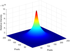
Figure 5. Plot of the derived scattering point spread function,  .
.
Download figure:
Standard image High-resolution image2.5. X-ray focal spot size and noise
X-rays do not originate from a single point source but over an area which is termed the x-ray focal spot. The size of the x-ray focal spot can limit the spatial resolution of projections at high geometric magnification. To take this into consideration the x-ray source is modelled as a circle with a diameter of 10 µm. Multiple rays are traced from randomly generated points within this circular spot to randomly generated points within each pixel and the results averaged, this is to take into consideration partial volume effects where the properties of different materials are averaged within a single pixel. The adopted focal spot model is simple to implement but deviates from the real case somewhat; studies have shown micro-focus x-ray spots to be approximately Gaussian in shape [23]. However, for the measurement task considered the geometric unsharpness due to the focal spot size is found to be 0.169 mm which is less that the detector pixel size (0.2 mm), so in this case the detector pixel size is likely to limit the spatial resolution of the projections and the precise shape of the focal spot is not likely to be a dominant factor, thus the simplified model adopted should suffice.
Projections are superimposed with Gaussian noise, the standard deviation of the noise is proportional to the square root of a given pixel value, this relationship is plotted in figure 6 based on the attenuation measurements from section 2.3. This relationship is found because x-ray detection is a counting process and therefore follows a Poisson distribution [5]. For a large number of events the Poisson distribution approximates a Gaussian distribution. The noise model is therefore written:

where  is a pixel value and
  is a random number drawn from a normal distribution with a zero mean and a standard deviation equal to
  , where
  and
and  are estimated from the least-squares line fitted to the data plotted in figure 6.
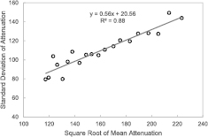
Figure 6. Graph showing how the parameters of the noise model are estimated.
Download figure:
Standard image High-resolution imageThe remaining simulated scan settings are as follows: the detector is 2000 × 2000 pixels with a pixel size of 0.2 mm, 2048 projections are simulated and the geometric magnification is ×17.9. These settings are based on those chosen at the University of Padova for real XCT scans of the PFG. The simulation is validated by comparing measured and simulated attenuation values of borosilicate glass up a thickness of 7 mm (the maximum path length through the object), the difference without scatter does not exceed 1% whilst the difference with scatter does not exceed 5%. An exemplary simulated projection of the PFG is shown in figure 7 alongside a simulated scatter signal.
Figure 7. (A) Simulated x-ray intensity image of the PFG. (B) Line profile across central pixel row of A. (C) Simulated scatter image of PFG. (D) Line profile across central pixel row of C.
Download figure:
Standard image High-resolution imageThe simulated scatter signal shown in figure 7 differs somewhat from scatter signals presented in other simulation-based work, namely because a high intensity signal is found in regions of the detector that the object does not occupy. This high intensity signal in unoccupied regions of the detector is due to veiling glare: the spread of x-ray and optical photons in the scintillation layer of the x-ray detector. The reason this signal is larger in areas surrounding the object is because this is where the highest x-ray flux falls on the detector leading to more scatter due to veiling glare. The scatter signals presented here closely follow the experimentally derived scatter signals of Schorner et al [24] Perterzol et al [25] and Lifton et al [10].
2.6. Beam hardening correction
Beam hardening is corrected using the linearization method [26, 27]. Polychromatic attenuation with and without scatter is plotted against monochromatic attenuation and 3rd order polynomials are fitted to the resulting curves. These polynomials are used to convert polychromatic attenuation ( values) to monochromatic attenuation (
 values) for each pixel of each projection, thus correcting for beam hardening. Two corrections are derived: one for attenuation values with scatter and one for attenuation values without scatter, the coefficients of each polynomial are given as follows, respectively:


2.7. Reconstruction, surface determination and geometry fitting
Reconstruction is performed using the Volume Graphics VGStudio MAX 2.2 (Volume Graphics GmbH, Heidelberg, Germany) implementation of the Feldkamp–Davis–Kress algorithm [28]. Projections are first filtered with a Shepp–Logan filter and then backprojected into the reconstruction volume. The data is reconstructed into a 2000 × 2000 × 2000 voxel volume as 8 bit integers, with a voxel size of 11 µm.
Surface determination is performed using both the ISO50 method and the advanced (local) method in Volume Graphics VGStudio MAX 2.2. The default settings are used for both surface determination methods. Inner and outer cylinders are fitted to the surface data using the default Gaussian best-fit option. Planes are fitted to the end faces of each cylinder to evaluate the cylinder lengths in accordance with the CT Audit measurement procedure [29]. CT images and a volume rendering of the reconstructed data are shown in figure 8.
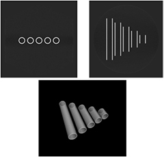
Figure 8. CT images and volume rendering of the reconstructed data.
Download figure:
Standard image High-resolution image3. Results
3.1. ISO50 surface determination
The cylinder length measurement errors for each simulation condition are plotted in figure 9 as evaluated via the ISO50 surface determination method. The measurement errors are in the order of ±1 µm which is approximately one tenth of the voxel size. The error bars represent the standard deviation of the errors of the 5 different length cylinders of the PFG.
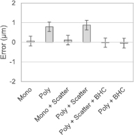
Figure 9. Length measurement errors, evaluated with the ISO50 surface determination method.
Download figure:
Standard image High-resolution imageThe cylinder length measurement results in figure 9 show that polychromatic data results in larger dimensions than monochromatic data, and that scatter has no significant influence on the length measurement results.
The measurement errors for the outer and inner diameters of the cylinders are plotted in figures 10 and 11 respectively as evaluated via the ISO50 surface determination method, the errors are again within one tenth of the voxel size.
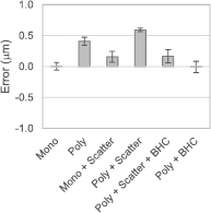
Figure 10. Outer diameter measurement errors, evaluated with the ISO50 surface determination method.
Download figure:
Standard image High-resolution image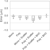
Figure 11. Inner diameter measurement errors, evaluated with the ISO50 surface determination method.
Download figure:
Standard image High-resolution imageThe outer diameter measurements in figure 10 show the following trends:
- Polychromatic data results in larger dimensions than monochromatic data.
- Scatter contaminated data results in lager dimensions than scatter free data.
- BHC leads to measurement results similar to the monochromatic data.
- Applying BHC to scatter contaminated data does not yield the same result as applying BHC to scatter free data.
The inner diameter measurements in figure 11 show the following trends:
- Polychromatic data results in smaller dimensions than monochromatic data.
- Scatter contaminated data results in smaller dimensions than scatter free data.
- BHC leads to measurement results similar to the monochromatic data.
- Applying BHC to scatter contaminated data does not yield the same result as applying BHC to scatter free data.
Thus both beam hardening and scatter cause outer dimensions to increase in size and inner dimensions to decrease in size. This opposing relationship is in agreement with previous experimental studies on the influence of beam hardening and scatter on dimensional measurements. The reason that inner and outer dimensions respond in opposition to scatter and beam hardening is due to the opposing direction of the grey value gradient evaluated by the 3D edge detection algorithm used for surface determination, a detailed explanation of this influence can be found in references [9, 10]. Note that in all cases the scatter contaminated polychromatic data leads to the largest measurement errors.
3.2. Local surface determination
The cylinder length measurement errors for each simulation condition are plotted in figure 12 as evaluated via the advanced surface determination method. All errors are within ±0.5 µm, which is approximately one twentieth of the voxel size.
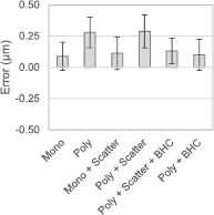
Figure 12. Length measurement errors, evaluated with the local surface determination method.
Download figure:
Standard image High-resolution imageThe cylinder length measurement results in figure 12 show that polychromatic data results in larger dimensions than monochromatic data, and that scatter has no significant influence on the measurement results.
The measurement errors for the outer and inner diameters of the cylinders are plotted in figures 13 and 14 respectively as evaluated via the advanced surface determination method.
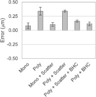
Figure 13. Outer diameter measurement errors, evaluated with the local surface determination method.
Download figure:
Standard image High-resolution image
Figure 14. Inner diameter measurement errors, evaluated with the local surface determination method.
Download figure:
Standard image High-resolution image
The outer diameter measurements in figure 13 show the following trends:
- Polychromatic data results in larger dimensions than monochromatic data.
- Scatter has no significant influence on the measurement results other than when a BHC is applied: applying a BHC to scatter contaminated data does not yield the same result as applying BHC to scatter free data.
The inner diameter measurements in figure 14 show the following trends:
- Polychromatic data results in smaller dimensions than monochromatic data.
- Scatter has no significant influence on the measurement results.
Thus beam hardening is the dominant influencing factor when the advanced surface determination method is used. Comparing the measurement results for the ISO50 and advanced surface determination methods, the latter is more robust to the influence of scatter and beam hardening and will therefore lead to lower uncertainty measurements. However, when beam hardening and scatter are corrected for, the ISO50 method leads to measurement errors that are comparable to the advanced method.
4. Discussion
The results show that both scatter and beam hardening influence the measurement results when evaluated using the ISO50 surface determination method, a difference of 0.2 µm is found between the BH and BH + scatter measurements of the outer cylinder diameters. However, when the local surface determination method is used, only beam hardening is a significant influencing factor, a negligible difference of 0.002 µm is found between the BH and BH + scatter measurements. It is doubtful that the latter result can be generalised, since the scatter signal generated by the PFG is likely to be much smaller than that of large metallic workpieces, such workpieces typically need to be scanned at low geometric magnification and with higher x-ray energies, both of which will result in much larger scatter signals than those considered here. A low geometric magnification means a small object-to-detector distance, so forward scattered x-rays are more likely to reach the detector due to geometric considerations. At higher x-ray energies Compton scattering becomes more dominant than photoelectric absorption, so more x-rays are scattered then absorbed. Furthermore, the probability of Compton scattering increases with material density, it would therefore be expected that a dense metallic part would generate a large scatter signal than a lower density material.
The results show that applying a BHC to scatter contaminated data can be less effective at reducing measurement errors due to beam hardening than applying a BHC to scatter free data, thus it is recommended that scatter is corrected prior to applying a BHC. Previous work showed that applying a BHC increases measurement errors [12]. It is suggested the reason BHC lead to larger measurement errors in reference [12] is that scatter was not considered prior to applying the BHC, and a single material BHC was applied to a multi-material object: a dedicated multi-material BHC is required for this purpose [30].
When the PFG was measured as part of the CT Audit the participant's measurement results displayed a clear pattern: the outer diameters of the cylinders were systematically measured too large whilst the inner diameters of the cylinders were measured too small [31]. This effect could be explained by the presence of beam hardening in the data. However, some participants applied a beam hardening correction to their data and the systematic errors remained. The results from the present study show that this residual error may be due to the presence of scatter in the data. This explanation should be further tested by applying both scatter and beam hardening correction to measured data of the PFG.
A plethora of scatter and beam hardening corrections have been proposed in the literature but not many of them have been tested in the context of XCT for dimensional metrology. In previous work the beam stop array scatter correction method was shown to lead to reduced measurement errors [10]. The simplest approach to minimise scatter and beam hardening is through good measurement setup. A large object-to-detector distance will help to reduce scatter as it will reduce the intensity of the scattered x-rays that fall incident on the detector since x-ray intensity follows the inverse square law. Collimating the source to irradiate only the scanned object will prevent the x-ray beam from interacting with other objects in the CT system, such as the cabinet, mechanical axes and the detector housing, all of which can generate scatter signals that will degrade image quality. Collimating the cone-beam to reduce the area of the detector that is irradiated will also reduce the amount of internal detector scatter generated (veiling glare). To reduce beam hardening, sufficient source pre-filtration should be used. Other hardware-based approaches include anti-scatter grids and post-object filtering. A pre-filter is a piece of material placed between the x-ray source and the detector, whilst a post-filter is a piece of material placed between the object and the detector. A difference in results obtained from these two filtering methods is found because the filter can act as an additional scattering source, in which case it is better to use a pre-filter due to the increased air-gap. On the other hand, a post-filter may absorb scattered x-rays that have been generated by the object, thus reducing the total scatter signal. The advantages and disadvantages of all of these strategies should be evaluated for dimensional XCT in future work.
The results of this study build upon and support a previous experimental-based study on the influence of scatter and beam hardening in XCT for dimensional metrology [10]. In the previous study the measurement uncertainty due to scatter and beam hardening was evaluated experimentally. A simulation-based approach to evaluate uncertainty contributors is an appealing option given the greater control over influencing factors and the potential to evaluate multiple factors simultaneously [32]. However, great care must be taken to sufficiently validate all aspects of the simulation against the XCT system to be modelled. In this work each part of the simulation has been driven by experimental data, furthermore, the simulated attenuation values have been validated against experimental values, only after validation can the simulation results be relied upon. The development of comprehensive XCT simulation tools for measurement uncertainty evaluation should be considered in future work, such tools will clearly be very computationally expensive, but can be tailored for implementation on graphics processing units which are well-suited for highly parallel computing tasks. It may be the case that evaluating measurement uncertainty through experimental means is no faster than a simulation-based approach, and at present the alternative analytical approach to XCT measurement uncertainty evaluation is not receiving much research attention.
5. Conclusions
This work has investigated the influence of scatter and beam hardening on dimensional measurements evaluated from simulated x-ray CT data. For the measurement task considered, both scatter and beam hardening were found to influence dimensional measurements when evaluated using the ISO50 surface determination method. On the other hand, only beam hardening was found to significantly influence dimensional measurements when evaluated using an advanced surface determination method. The results showed that the ISO50 surface determination method led to measurement errors of less than one tenth of the voxel size, whilst the advanced surface determination method led to measurement errors of less than one twentieth of the voxel size for measurements of length and size. In future work an experimental study on the influence of scatter and beam hardening on the PFG should be conducted to further validate this simulation-based work. Furthermore, the influence of different scatter correction methods on the accuracy of CT-based dimensional measurements should be investigated.
Footnotes
- 3
This rule may be violated when the energy of an x-ray photon is equal to the binding energy of the K shell electrons of an atom.