

Abstract
In this article we provide an overview of widely used methods to measure the mean and fluctuating components of the wall-shear stress in wall-bounded turbulent flows. We first note that it is very important to perform direct measurements of the mean wall-shear stress, where oil-film interferometry (OFI) provides the highest accuracy with an uncertainty level of around 1%. Nonetheless, several indirect methods are commonly used due to their straightforward application and these are reviewed in the light of recent findings in wall turbulence. The focus of the review lies, however, on the fluctuating wall-shear stress, which has over the last decade received renewed interest. In this respect, it is interesting to note that one near-wall feature that has received attention is the so-called backflow event, i.e. a sudden, strong short-lived reverse-flow area, which challenges measurement techniques in terms of temporal and spatial resolution, as well as their dynamic range and multi-directional capabilities. Therefore, we provide a review on these backflow events as well as commonly used techniques for fluctuating wall-shear-stress measurements and discuss the various attempts to measure them. The review shows that further development of the accuracy and robustness of available measurement techniques is needed, so that such extreme events can be adequately measured.
Export citation and abstract BibTeX RIS

Original content from this work may be used under the terms of the Creative Commons Attribution 4.0 license. Any further distribution of this work must maintain attribution to the author(s) and the title of the work, journal citation and DOI.
1. Introduction
The main difficulty in obtaining accurate measurements of turbulent flows is the fact that the fluid velocity changes both in space and time covering a broad range of spatial and temporal scales. Typically the instantaneous velocity vector  is decomposed into the sum of mean (
 ) and fluctuating (
 ) components, following the so-called Reynolds decomposition [1]. In addition to the great importance of accurately determining the mean wall-shear stress
for engineering purposes (for instance, the viscous drag amounts to around 50% of the total drag in commercial aircraft [2] and even more in ships and submarines [3]), this quantity also has highly relevant implications in the scaling and asymptotic behavior of mean and fluctuating profiles in wall-bounded turbulent flows [4–7]. Note that µ is the dynamic viscosity of the fluid, (dU/dy)w is the wall-normal gradient of the mean streamwise velocity evaluated at the wall and the overbar indicates the averaging operator, which will be used henceforth to distinguish the mean from its fluctuating component. One important property of wall-bounded turbulent flows is the fact that they are governed by two different length scales [8], i.e. the so-called viscous length  (where ν is the fluid kinematic viscosity and
  is the friction velocity, defined in terms of the wall-shear stress and the fluid density ρ), which applies in the inner region close to the wall; and the scale in the outer region (where inertial effects are dominant) which is typically the boundary-layer thickness δ (or equivalently the radius or half-height in the case of internal flows). The so-called viscous scaling considers
  and
and  as velocity and length scales, respectively and is denoted by the superscript '+'. The inner-scaled mean velocity profile
  exhibits an overlap region (where the inner and outer descriptions of the profile are valid for
  and
and  ), which is described by a logarithmic velocity profile, henceforth log-law [6, 9–11]:
In this equation, κ is the so-called von Kármán coefficient and B is the log-law intercept. Note that there is no agreement in the turbulence community regarding the value of κ and its universality; while in some studies it is claimed that κ is flow-dependent [12], other authors claim that it is universal, at least in boundary layers, pipes and channels [6]. Other recent works argue that the universality of κ is recovered when accounting for the effect of streamwise pressure gradients [13] or by considering two different logarithmic laws in the overlap region [14]. Values close to κ = 0.38 and B = 4.17 are currently accepted for zero-pressure-gradient (ZPG) turbulent boundary layers (TBLs)—see for instance references [15–17]—and recent experiments in pipe flow at high Reynolds number [18] as well as direct numerical simulations (DNS) in channel flow [11] have reported similar values. As will be discussed below, the mean velocity profile can be used to determine the mean wall-shear stress, although this method exhibits several drawbacks. The relevance of the von Kármán constant, in particular, becomes important in the context of turbulence modelling, cf the review by Spalart [19].
Another important quantity when assessing the characteristics of wall-bounded flows is the Reynolds-stress tensor, in particular the variance of the streamwise velocity fluctuations  . Its correct scaling has been a subject of debate, with certain authors proposing a mixed scaling [20] involving the product
  (where
  is the freestream velocity in external flows or equivalently an outer velocity scale for internal flows), and some analyses suggesting that the outer scaling with
  provides the best collapse of data in the outer region [4]. The work by Monkewitz and Nagib [21] on ZPG TBL data analysis shows that
  increases with
  when scaled in inner units in the near-wall region. This Reynolds-number dependence is in agreement with the recent particle-image-velocimetry (PIV) measurements by Willert et al [18] in a turbulent pipe flow up to a friction Reynolds number of
  (where
  ), which also exhibit an increasing value of the near-wall peak (located at a fixed inner-scaled location of around y+≃ 15) with
  . Direct-numerical-simulation (DNS) results and experimental studies in canonical flows, albeit at lower
  , also exhibit a clear Reynolds-number increase of the inner-scaled near-wall peak. However, this observation contradicts the view by Hultmark et al [22] and a series of results from the Superpipe in both pipe and boundary-layer flows utilizing nanoscale-sensing devices (NSTAPs) [23, 24]. In these studies the authors observed that the value of the near-wall peak becomes Reynolds-number independent for high-enough
  [25]. Inconsistencies in the results from the Superpipe have been raised by Örlü and Alfredsson [26]1.
Related to the scaling of the near-wall peak of the streamwise variance profile is also the scaling of the streamwise turbulence intensity, which in the limit of y → 0 approaches the magnitude (i.e. rms value) of the fluctuating wall-shear stress [28, 29]:
The instantaneous distribution of the wall-shear stress (and hence its magnitude) also reflects the structure of the boundary layer close to the wall. Compelling evidence from DNS data sets have over the last decade established a clear Reynolds-number dependence of  [30–33], which—as is evident, for example, from two-dimensional spectral maps of the fluctuating wall-shear stress [29, 34]—is a result of the footprints of the outer-layer structures on the near-wall region [35]. These findings go along with the established failure of inner scaling for the Reynolds normal stresses and the
  -dependence of the higher-order moments of the velocity fluctuations [36–38].
There is also some uncertainty in the turbulence community regarding the emergence of an outer peak in the streamwise velocity fluctuation profile of canonical wall-bounded flows, while its existence in adverse-pressure-gradient boundary layers is well established [39]. For canonical wall-bounded flows some authors claim that at sufficiently high Reynolds numbers such an outer peak emerges in the logarithmic layer and eventually reaches values larger than that of the inner peak [40], while other studies [41] suggest that the velocity fluctuations in the outer region increase, but remain beneath the amplitude of the inner peak. An alternative view [21] proposes that although the outer-region fluctuations increase with  , they only reach the value of the near-wall peak for infinite Reynolds number. Note that the complexity of wall-bounded turbulent flows, combined with the number of open questions regarding the behavior at progressively higher
  , highlight the importance of being able to measure, in an accurate and robust way, the wall-shear stress.
Two trends are important to mention here that make the precise knowledge of the fluctuating wall-shear stress crucial: On the one side, flow-control efforts focusing on skin-friction drag reduction. These are either aimed at interfering with the near-wall cycle, i.e. the regeneration process [42], or at the large-scale structures in the outer region that are known to modulate the small-scale structures near the wall and thereby the wall-shear-stress fluctuations [43, 44]. Besides these two main themes in turbulent flows, fluctuating and mean wall-shear-stress measurements are crucial for the detection of the transition from laminar to turbulent flow as well as the identification of (incipient) flow separation. Fluctuating wall-shear-stress measurements are also used to detect abnormal blood flow to predict arterial diseases [45, 46]. On the other side, the existence of sudden, rare and strong events, so-called extreme events, which are manifested as strong wall-normal fluctuations, critical points or backflow events in the viscous sublayer [37]. The existence of the latter extreme events, foremost established via DNS, has recently become a test case for measurement techniques and will continue to serve as a challenge for novel measurement techniques.
The present article is organized as follows: we start by discussing the common techniques used to measure the mean wall-shear stress in section 2; in section 3 we describe the common methods employed to measure the fluctuating wall-shear stress; in section 4 we provide a description of the near-wall extreme events in wall-bounded turbulence, with particular emphasis on backflow events and critical points and assessment of the various methods available to measure them; and finally in section 5 we summarize the article and provide an outlook.
2. Mean wall-shear-stress measurements
There are a number of methods to experimentally determine the wall-shear stress, each of them exhibiting different levels of complexity and accuracy. We restrict ourselves here to commonly used techniques and refer to classical review papers for a more detailed overview [47–50]; for a chronological overview see also reference [51]. In the following, we discuss indirect techniques (where the wall-shear stress is inferred from another measured quantity) based on the mean velocity profile, the heat-transfer rate from the wall to the fluid and pressure measurements, as well as direct methods such as floating elements and oil-film interferometry (OFI).
2.1. Techniques based on the mean velocity profile
We first discuss the methods based on the mean velocity profile, which has traditionally been obtained by means of Pitot tube and hot-wire anemometry probes. The former has the advantage of allowing flow measurements close to the wall, although it requires a number of corrections associated with the effects of shear, wall proximity and turbulence, as thoroughly reviewed and discussed in references [52, 53]. When it comes to hot-wire anemometers, on the one hand they exhibit much better frequency response (which allows measurement of velocity fluctuations), while on the other hand they have problems related to the determination of the absolute wall position due to probe deflection as well as spatial-resolution effects due to the finite wire length [5, 53, 54] and, in particular, additional heat conduction due to the presence of the wall [55]. In principle, if high-quality measurements are available very close to the wall, the wall-shear stress can be determined from the fact that in the viscous sublayer (i.e. up to y+≃ 5) the mean velocity profile follows a linear profile:  . However, given the limitations of most experimental techniques to determine the velocity very close to the wall, typically this method cannot be reliably employed and therefore it is necessary to use the data further from the wall. This is problematic, because there are still a number of open questions regarding the Reynolds-number evolution of the inner-scaled mean velocity profile beyond the viscous sublayer. Therefore, if certain assumptions must be made in order to determine
  , there is a risk that the resulting profile may just confirm the underlying hypotheses, i.e. circular logic (see the related discussion regarding the overlap region in reference [56]).
One of the methods relying on assumptions to determine  from the mean velocity profile is the so-called Clauser chart/plot method [57]. This approach is based on the premise that the overlap region of the mean velocity profile follows the logarithmic law (2), which although widely established and accepted in the community, relies on certain values of the log-law constants. In particular, the Clauser-chart method relies on the values κ = 0.4 and B = 4.9, which were determined in the 1950s by Clauser [57] and as discussed above might not be the values that most accurately represent the data presently available. Despite the log-law parameters having been assumed constant for decades, the actual values used in conjunction with the Clauser chart/plot method have varied from author to author and have often been adjusted depending on flow case and Reynolds-number range [58]. Furthermore, there is an ongoing debate not only about the values of these constants [59], but also regarding their universality for different types of flows [12]. In addition to this, certain authors such as Tavoularis [60] indicate that there is some degree of subjectivity when using the Clauser chart, for instance regarding the selected limits of the overlap region, which significantly affect the obtained results as also reviewed in reference [5]. The limitations of the Clauser chart motivated the need to use direct methods to determine the wall-shear stress [61], in order to avoid alternative assumptions that may hinder us from obtaining the true behavior of
  . The value of κ is in fact also relevant in the context of turbulence modeling, where most models rely on the value of this constant [19, 62]. Moreover, the value of κ is also present in the equation defining the evolution with the Reynolds number of the skin friction, which can be obtained by matching the equations for the logarithmic law in inner and outer scaling:
This further shows the problems arising from determining the skin friction through prescribed values of the logarithmic-law constants. Furthermore, since the results also depend on the limits of the logarithmic region [5], a number of authors have proposed functional forms of the mean velocity profile that blend into the viscous sublayer and wake regions [16, 49, 63, 64], although these typically include a larger number of fitting constants, which might also impact the accuracy of the determined wall-shear stress (for a comparison of various velocity-profile descriptions, see reference [65]). Nonetheless, these so-called composite velocity profiles have become the preferred, albeit indirect, method to determine the wall-shear stress, in particular, when sublayer data are not at hand and/or the Reynolds number is not sufficiently high that a clear and large enough logarithmic region is established.
Another method relying on mean velocity measurements is the use of the von Kármán momentum theorem, extended to account for turbulent terms [66, 67], which, however, exhibits the problem of requiring a well-resolved streamwise resolution to obtain reasonable wall-shear-stress results. Although these additional Reynolds-normal stress terms are found to account for only up to 2% compared to the leading-order terms in the case of ZPG TBL flows [68], these methods are, nonetheless, preferable, particularly in non-canonical flows, where the logarithmic region and hence its constants are influenced by external factors, such as in flows with pressure gradients. Since gradients in the streamwise direction need to be evaluated it is best suited for measurement campaigns with a well-resolved streamwise direction, as for instance given through particle image velocimetry (PIV) measurements, but also detailed hot-wire or laser-Doppler velocimetry measurement campaigns with sufficient streamwise measurement locations [69, 70]. The main difficulty in the utilization of this method is its sensitivity to inaccuracies in computing the streamwise gradient terms. An alternative method based on the so-called Fukagata, Iwamoto and Kasagi (FIK) identity [71] modifies the momentum integral such that streamwise derivatives are replaced through wall-normal profiles of the mean streamwise velocity and Reynolds shear stress, so that the evaluation can be performed at only one streamwise position [72, 73], which is preferable in particular for single-point measurements.
2.2. Techniques based on the heat-transfer rate to the fluid
Other methods to determine the wall-shear stress involve exploiting the connection between the heat-transfer rate to the fluid and the wall-shear stress. Some of the most popular methods based on heat transfer are surface hot films and wall-mounted hot-wire probes [28, 74–76]. The former are heated metallic elements placed at the wall, with which according to Tavoularis [60] it is possible to develop a King's-law type of relation between the voltage of the sensor and  . Note that this sensor only works well if the thermal conductivity of the fluid is larger than that of the wall material. Since this is not the case for air, the latter method, i.e. the wall-mounted hot wire, is usually preferred for this fluid. This technique is based on placing a hot wire mounted at the wall, measuring within the viscous sublayer. The measured voltage of the probe is then directly calibrated against the mean wall-shear stress [50]. While some groups prefer calibrations against, for example, laminar channel flows [77, 78], others prefer to calibrate the probe in a turbulent flow [28]. A further development of wall-mounted hot wires, so-called surface hot wires, combines the advantages of hot-wire anemometry and flush-mounted sensors, i.e. the measured data retains the frequency response of a hot wire, while avoiding reliance on the viscous-sublayer scaling. This is accomplished through usage of a flush-mounted, hot-wire sensor, in which the hot wire is installed over a small cavity and is flush with the wall, thereby avoiding direct contact and minimizing conduction from the hot wire to the sensor substrate [79, 80].
2.3. Techniques based on pressure measurements
Another category of methods includes the ones that exploit pressure measurements to determine the skin friction. A straightforward example of this is the global force balance in turbulent channel and pipe flows relating the streamwise pressure gradient dP/dx to the wall-shear stress through
where H and D denote the full height of the channel and the diameter of the pipe, respectively. Note that equation (5) only holds in fully developed flows which are uniform in the spanwise or azimuthal direction, as is the case in channels or pipes. Nonetheless, any experimental realization of a turbulent channel flow necessarily includes side walls and is therefore denoted with the term duct. We define the aspect ratio of a duct as its total width divided by its total height and only for aspect ratios larger than around 10 a spanwise homogeneous region is observed at the duct centerplane [81]. It is important to note that even in a duct wide enough to exhibit a spanwise homogeneous region at the core, equation (5) would not yield the centerplane wall-shear stress due to the contribution of the side walls to the pressure drop [82–84]. Since the local friction velocity at the centerplane needs to be used to scale turbulence quantities [85], it is essential to perform direct measurements of the wall-shear stress [86], for instance through the oil-film interferometry (OFI) method [87] discussed in section 2.5. The only flow geometry where equation (5) is directly applicable for global and local wall-shear-stress measurements is therefore a fully developed pipe flow, which explains why recent large-scale facilities to obtain high Reynolds number are predominantly pipe flows [88–91].
Another method based on the pressure is to employ a Preston tube, which is essentially a Pitot tube placed at the wall. Based on the analysis by Preston [92], it is possible to relate the wall-shear stress and the measured pressure difference Δp based on a number of calibration parameters, where the most widely used calibration is the one by Patel [93]. An important aspect to keep in mind is that the inner-scaled tube diameter increases with Reynolds number (despite the fact that it is fixed in physical units) and therefore different calibration parameters are needed for various Reynolds-number ranges [93, 94]. Note that this technique provides reasonably accurate results of the mean wall-shear stress, but it relies on prescribed values of κ and B, a fact that precludes this method from providing independent  measurements for scaling studies. A variation of the Preston tube is the so-called Stanton tube, which is smaller and has a better frequency response. Several calibration parameters were provided by East [95] and the limitations of this device were discussed by Haritonidis [49]. A third device based on pressure measurements is the sublayer fence first described in reference [96], in which simply the pressure difference upstream and downstream of a razor-blade fence is measured, hence the technique is also capable of indicating backflow. The sublayer fence is designed to remain within the viscous sublayer and is relatively more sensitive than the Stanton tube [47]. Designs based on microelectromechanical systems (MEMS) are also able to provide time-resolved information [97, 98].
2.4. Floating elements
Wall-shear-stress measurements in rough TBLs typically rely on indirect methods. However, Aguiar Ferreira et al [99] have recently proposed a technique to perform direct friction measurements in rough TBLs. This technique is based on the floating element, which is essentially a force balance placed in a cavity with a floating surface. By directly measuring the force exerted by the incoming flow on the floating element, it is possible to obtain the wall-shear stress. Despite the limitations of the traditional floating-element device [47, 100], the design proposed by Aguiar Ferreira et al [99] replaces one set of flexures by single bending-beam transducers, which allow monitoring of the streamwise load and can therefore obtain reliable wall-shear-stress measurements both in smooth and rough TBLs. Alternatively, large-scale floating elements with large surface areas are preferred in order to improve the signal-to-noise ratios of traditional floating-element techniques [101]. Another point that becomes important when dealing with rough surfaces is the contribution to the fluctuating wall-shear stress and wall pressure from the pressure drag on the roughness elements. As shown in reference [102] the high-frequency region of these quantities scales similarly to their smooth-wall counterpart, when adjusted to exclude the pressure drag on the roughness elements.
2.5. Oil-film interferometry (OFI)
Most of the methods discussed above rely on given values of the coefficients in the logarithmic region (2), or do not provide direct measurements of the wall-shear stress. One method that solves these two problems is oil-film interferometry (OFI), which was already proposed in the 1970s by Tanner and Blows [103], but became widely used in the context of wall-bounded turbulence research in the 1990s [104]. This technique is based on placing one or more oil drops on the wall and as the incoming stream forms a thin oil film, it is possible to develop a correlation between the wall-shear stress and the film thickness. In practice, the oil film is illuminated with a monochromatic light (usually a sodium lamp) and because the film thickness defines the total path length of incoming light within the film, it is possible to observe constructive and destructive interferences (between the light ray reflected from the film surface and the one reflected from the bottom wall) leading to light and dark fringes on the wall, respectively. These fringes are captured with a camera during the experiment, leading to a number of images exhibiting the Fizeau interferometric fringes shown in figure 1.
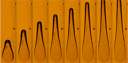
Figure 1. Development of an oil film during the experiment, exhibiting the interferometric pattern. The flow is from bottom to top and time progresses from left to right.
Download figure:
Standard image High-resolution imageThe interferograms can be analyzed in various ways with the aim of obtaining the velocity of the fringes. For instance, the XT method proposed by Janke [105] is based on analyzing the varying position of the fringe with time within a manually selected interrogation line, so as to determine its velocity. With the fringe velocity, one needs to use the difference in thickness between two consecutive dark fringes (which can be obtained based on optical considerations [106]) to determine the wall-shear stress. The XT method was for instance used by Österlund et al [15] to independently measure the skin friction and draw conclusions regarding the mean velocity profile in canonical ZPG TBLs. An alternative is to compute the mean peak distance of the interferometric pattern through local and global wavelength estimation methods. This approach was found to be more accurate than the XT method by Vinuesa et al [86], together with the accurate method based on the Hilbert transform by Chauhan et al [107]. A number of extensions to this analysis have been proposed by Segalini et al [108], who emphasized the importance of obtaining an accurate calibration of the oil viscosity in order to minimize the error in the determination of  . A step-by-step description of the process is provided by Vinuesa and Örlü [109] and a detailed analysis of the uncertainties in the OFI method was provided by Rezaeiravesh et al [110]. Note that OFI is the most accurate technique to measure the mean wall-shear stress and it is able to provide error levels below 1% [108, 110], although larger uncertainties are reported in earlier studies as summarized in reference [111]. Note that although OFI measurements are mostly conducted with monochromatic light, a white light source can be used as well [112], but is still foremost used for quantitative analyses of 3D flows [113]. While OFI is the method of choice for mean wall-shear-stress measurements, it is not possible to measure the fluctuating component of the wall-shear stress, which is another very relevant quantity in wall-bounded turbulence. Therefore, a variety of methods have been developed to accurately measure this quantity and we discuss these next.
3. Instantaneous wall-shear-stress measurements
Having discussed the most common and widely used techniques for mean wall-shear-stress measurements, in this section we summarize the most widely used methods to measure the wall-shear-stress fluctuations. Note that the fluctuating wall-shear stress is another very relevant quantity in wall-bounded turbulence, since it reflects the influence of the large-scale motions in the outer region on the structures near the wall [29]. We next discuss the following techniques: hot-wire and hot-film anemometry (HWA and HFA), laser Doppler anemometry (LDA), particle image velocimetry (PIV), molecular tagging velocimetry (MTV) and micro-pillar shear-stress sensors (MPS3). Other less common techniques, e.g. electrochemical techniques (which exploit the similarity between mass and momentum transfer [114]), have been omitted here for brevity, although there are some recent works that deserve attention [115, 116].
3.1. Hot-wire and hot-film anemometry (HWA and HFA)
Since most classical reviews on wall-shear-stress measurements provide an in-depth review on thermal-anemometry-based techniques, it will suffice for us to refer to only a few of these classical references [48, 49, 117, 118] and merely highlight why these cannot be used for accurate fluctuating wall-shear-stress measurements (cf references in reference [119]). As will be outlined in section 4 and documented in various studies based on DNS results, the fluctuating streamwise velocity approaches zero velocity not only within the viscous sublayer, but even beyond for increasing  and complex flows, i.e. with adverse pressure gradients. As illustrated in the probability density distribution of the streamwise velocity component in figure 2, the low-speed fluctuations reach velocities that are influenced by free convection beyond the viscous sublayer. Furthermore, due to the directional insensitivity of hot wires and hot films, the measured fluctuating wall-shear stress will inherently be blind to reverse flow events [37] and rectify the hot-wire signal. Hence, wall-mounted hot-wire probes and surface-mounted hot-film probes have recently mainly been used as sensors for flow-control purposes [120] or to measure large-scale fluctuations related to amplitude modulation studies [121, 122].

Figure 2. Mean streamwise velocity over wall-normal position scaled in inner variables, U+ vs. y+, (white line) plotted above the probability density function (pdf) of the instantaneous streamwise velocity from a DNS of a ZPG TBL flow at  2500 [68]. Reprinted by permission from Springer Nature Customer Service Centre GmbH:Nature, Experiments in Fluids, [31], Copyright © 2011, Springer Nature.
Download figure:
Standard image High-resolution image3.2. Laser Doppler anemometry (LDA)
Some of the earlier studies focused on using laser Doppler anemometry (LDA) to measure the wall-shear stress, including those by Naqwi and Reynolds [123] and Fourguette et al [124]. The idea, which is based on the laser Doppler velocimetry (LDV) technique for velocity measurements, is to seed particles on the flow and illuminate a certain region from below the test section with a laser beam with wavelength λ. This beam is passed through a diffractive lens with two narrow gaps separated by a distance s. The seeded particles in the flow will scatter the beam light at the Doppler frequency fD and because the velocity profile in the viscous sublayer is linear, all the particles will scatter light at the same frequency. Using this principle, it is possible to show [125] that the wall-shear stress τw is directly proportional to λ, fD and the fluid dynamic viscosity µ and inversely proportional to s. This method is able to detect flow reversal, exhibits an excellent frequency response and does not require calibration. It is therefore a very good approach to measure the fluctuating wall-shear stress. However, this measurement technique has some limitations related to the behavior of the particles very close to the wall and may have problems related to particle seeding.
The comparably large measurement volumes in LDV experiments require corrections, in particular, in the immediate vicinity of the wall, as, for example, discussed in the seminal work by Durst et al [126] and reference literature [118, 127]2. A workaround to this problem is the laser Doppler profile sensor [129, 130], which can be considered as an extension of the LDV principle. Instead of one single-fringe system, two distinguishable superposed converging and diverging fringe systems are overlaid to create a mesh from which the particle position within the measurement volume can be determined, thereby increasing the spatial resolution by more than one order of magnitude compared to conventional LDV systems [131]. Turbulence statistics up to the fourth order in wall-bounded flows down to one viscous unit were found to agree well with DNS data sets with an accuracy superior to those of conventional LDV systems [132]. An extension to the above-mentioned laser Doppler profile sensors towards the simultaneous measurement of three components of velocity and position is described in reference [133]. Despite these favorable features, the technique is not yet an off-the-shelf measurement technique and further studies under more challenging conditions are needed to establish its applicability to fluctuating wall-shear-stress measurements.
3.3. Particle image velocimetry (PIV)
PIV measures the velocity of tracer/seeding particles that are naturally present or artificially added to a flow by recording two images of tracer particles—which are usually illuminated by a thin laser sheet—with a given short-time separation using a digital camera. During this short time the particles move a distance of the order of a few pixels, from which the local velocity of the particles can be determined. It is hence the quantitative counterpart of smoke visualizations. While planar PIV provides the velocity components in a plane, stereo PIV adds its out-off-plane component and tomographic/volumetric PIV provides all three velocity components in a 3D volume. While pointwise measurements such as those discussed in the previous sections provide higher-accuracy statistics, PIV has commonly been preferred for studying coherent structures or global flow features that require multi-point measurements. Recent advances in high-speed cameras and powerful high-repetition lasers have, however, contributed to the fast development of PIV, which increasingly constitutes an alternative to HWA and LDV in terms of turbulence statistics in wall-bounded flows [134, 135]. There is a vast amount of literature that is accessible in well-known textbooks [136, 137] and review papers focusing on different applications and specializations of PIV [138–143]. While initially mainly focused on structural information of the flow, improvements in post-processing techniques have also made it comparably accurate to HWA and LDV in wall-bounded turbulent flows including higher-order moments [144–146]. Nonetheless, it suffers from the same limitations as LDV, i.e. it relies on the assumption that the seeding/tracing particles do not exhibit a larger time lag than the smallest timescale of the flow of interest. When it comes to measurements in the viscous sublayer, a poor seeding density is also a problem and the scarcity of particles opened the door for particle tracking velocimetry (PTV). Over the last few years, PTV has provided detailed data within the viscous sublayer surpassing both HWA and LDV [147–149]. In particular, in conjunction with recent efforts to provide near-wall turbulence statistics at high Reynolds numbers (where LDV and HWA usually suffer from spatial-resolution issues), dedicated efforts with µPIV/PTV [150] and high-speed PIV [134, 135] have provided data that for the first time show a clear increase of the near-wall peak in the streamwise variance profile with increasing Reynolds number [18]. It is hence to be expected that PIV/PTV, in conjunction with the developments in high-resolution and high-speed cameras as well as high-repetition lasers, will continue to provide near-wall statistics and fluctuating wall-shear-stress measurements that are not accessible with the more traditional measurement techniques mentioned above. One of these recent developments is the Shake-the-Box (STB) [151] approach, which is a novel time-resolved tracking method for measuring densely seeded flows. This technique can be seen as 4D-PTV and has recently been used [152, 153] to provide measurements of the complete Reynolds-stress tensor within the viscous sublayer, including evidence of backflow events in ZPG TBL flows.
3.4. Molecular tagging velocimetry (MTV)
Although molecular tagging velocimetry (MTV) might not be the first measurement technique that comes to mind when one considers wall-shear-stress measurements, the first successful and direct measurements of velocity gradients in the viscous sublayer and thereby the wall-shear stress of turbulent flows were MTV measurements by Klewicki and Hill [154, 155]. MTV can be seen as the molecular counterpart of PIV [156], where instead of seeding particles, molecules are tracked. In the same sense as PIV can roughly be considered as the quantitative counterpart of smoke visualizations, MTV could be considered as the quantitative counterpart of hydrogen-bubble visualizations [157, 158], which—via flash-photolysis methods—provided the basis for the first visualization of the instantaneous velocity profile within the viscous sublayer half a century ago [159, 160].
One of the main limitations of LDV and PIV is that they rely on the assumption that the seeding/tracing particles do not exhibit a larger time lag than the smallest timescale of the flow of interest. This is, in particular, a problem for LDV and PIV measurements in flows with high accelerations (as is the case for shock waves or extreme events). Additionally, the immediate near-wall region and hence viscous sublayer suffer from reflections from the light source in case of glass or plexiglass surfaces as well as the poor seeding in this region (i.e. low data rates in the case of LDV). These shortcomings are inherently overcome by relying on molecules rather than (seeding) particles [161] through excitation of naturally present (or premixed) molecules that are turned into tracers. Different MTV mechanisms exist and they are known under various acronyms [162], but typically single- and multiple-line tagging are the most relevant to the measurements of wall-shear stress [163, 164]. These tagged regions of interest are then—similar to PIV—tracked and interrogated to determine the Lagrangian displacement and thereby the velocity vector [156, 162]. Blue lasers, ultraviolet (UV) light sources, are commonly used for these kinds of measurements [165].
While one- and two-component measurements have been common in the past [155, 163, 166], smooth and converged turbulence statistics with an accuracy comparable to that of HWA, LDV and PIV have only recently become available due to advances in high-resolution digital cameras, since the spatial resolution in MTV matches that of the camera resolution. For instance, experimentally obtained first- and second-order derivative profiles of the mean velocity profile could only recently be obtained via 1 C-MTV measurements in a turbulent channel that agree with DNS [164]. Despite these clear advantages compared to PIV, there are nonetheless similar shortcomings that become apparent when performing measurements in high-Reynolds-number wall-bounded flows. Insufficient spatial resolution is one obvious shortcoming and as for HWA [167, 168] and PIV [169, 170], in the case of MTV, the depth of focus (DOF) of the lens appears to have the same effect as a finite wire length in HWA [164]. One recent development to improve the spatial resolution is the utilization of the so-called (optical) Talbot effect [171], which generates very fine-structured illumination patterns. Advances in green lasers (towards high frequencies and high powers), which are predominantly used in experimental fluid dynamics laboratories, have also recently been possible to use for MTV through the utilization of caged dyes [171]. It is hence to be expected that MTV for the purpose of temporally and spatially well-resolved instantaneous wall-shear-stress measurements, and turbulence measurements in general, will continue to push the limits of velocimetry.
3.5. Micro-pillar shear-stress sensors (MPS3)
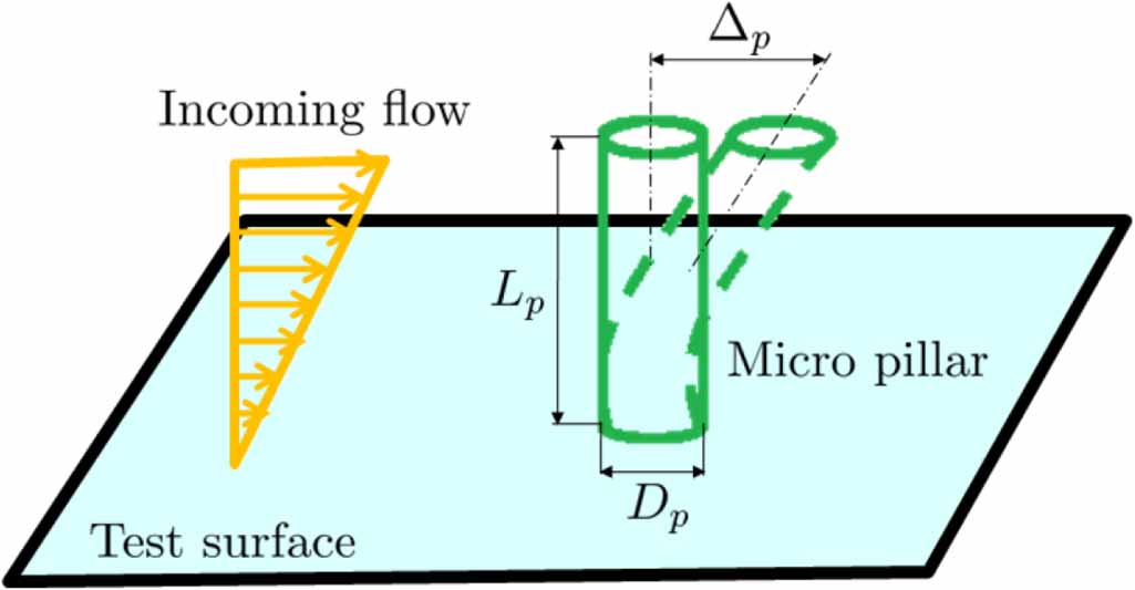
The micro-pillar shear-stress sensor (MPS3) is a technique specifically developed to accurately measure the fluctuating wall-shear stress. In this method, we consider an array of elastic micro-pillars placed at the wall and determine the wall-shear stress based on the pillar deflection caused by the incoming stream. In particular, this sensor allows us to determine the orientation of the wall-shear-stress vector, as highlighted by Brücker et al [172] and by Große and Schröder [173]. In figure 3 we show a schematic representation of the basic parameters relevant to this sensor. Assuming linear bending theory [174], the displacement of the pillar tip Δt can be related to the wall-shear stress through the following equation:
where Ep, Lp and Dp are the Young's modulus, length and diameter of the pillar, respectively. Note that turbulent flows are characterized by a wide range of spatial and temporal scales and therefore the micro-pillar motion will exhibit fluctuations which may reach frequencies of the order of kHz for the smallest scales. Different solutions have been proposed to account for such high-frequency fluctuating behavior, including the definition of a frequency-dependent added mass to model the sensor dynamics [175], or the development of dynamic-calibration methods [174]. The following partial differential equation describes the dynamic behavior of the micro-pillar:
where  is the stiffness of the micro-pillar, Δ(y, t) is the micro-pillar displacement at height y and instant t,
  and
and  are the reduced mass and damping coefficients, respectively, and F(y, t) is the excitation. The Strouhal number is calculated as
  , with f being the frequency of interest. Note that micro-pillars have an approximately constant transfer function below a particular frequency f0, i.e. in the range up to ≃ 0.4f0, where this frequency can be determined by solving an aeroelastic problem [176]. Another important aspect to keep in mind is the fact that the micro-pillar needs to be immersed in the viscous sublayer and this effectively limits the value of Lp to the order of microns depending on flow case and Reynolds numbers. This implies that optical systems and high-resolution cameras are required in order to accurately capture the micro-pillar movement. Typical spatial resolutions of this technique are of the order of 5 viscous units and shear stresses of around 0.01 N m−2 can be measured. The MPS3 sensor is an excellent technique to measure the fluctuating skin friction and extreme events close to the wall (such as backflows or critical points) have been studied with this method [177], as discussed next.

Figure 3. Schematic representation of a micro-pillar shear-stress sensor and relevant parameters.
Download figure:
Standard image High-resolution image4. Near-wall extreme events: the ultimate challenge
4.1. Characteristics of extreme events
A very relevant near-wall flow topology is the presence of regions of instantaneous reverse flow, also denoted by the term backflow event. These events in wall-bounded turbulence are of importance to understand the mechanisms of flow separation in steady [178] and unsteady [179] turbulent external flows, transitional flows [180], and in heat-transfer applications [181]. Despite their importance in a wide range of applications, their existence in wall-bounded turbulence was not completely confirmed until DNS studies focused on wall-shear-stress fluctuations. In fact, the occurrence of negative streamwise velocities in wall-bounded turbulence is a counterintuitive phenomenon. Eckelmann [182] stated in 1974 that 'with certainty, there are no negative velocities near the wall'. More recently, Colella and Keith [183] concluded that 'The probability density of wall-shear-stress fluctuations [...] exhibits no flow reversals at the wall.' Despite scarce evidence from experiments, these were ignored and assumed to be related to measurement uncertainties or noise. This changed after the DNS study of turbulent channel flows by Lenaers et al [37], who observed that although these events are very rare (their probability of occurrence is 0.06% at  ), they become more frequent and are observed up to higher wall-normal locations for increasing Reynolds numbers. Before the study by Lenaers et al [37], the aforementioned experimental campaigns by Eckelmann [182] and by Colella and Keith [183] based on hot-film sensors reported no evidence of negative velocities close to the wall. Probably the first experiments reporting the presence of backflow events were the LDV measurements by Johansson [184], who argued that additional research was needed in order to completely characterize these rare events to establish their existence beyond doubt. Another extreme near-wall event discussed by Lenaers et al [37] is the presence of very large wall-normal fluctuations, which produce high flatness and were documented experimentally by Xu et al [185], who performed LDV measurements.
According to Lenaers et al [37], the backflow regions are circular and have an approximate diameter of 20 viscous units, which is independent of the Reynolds number. They also reported that these backflow events are caused by oblique near-wall vortices, a fact that explains the strong spanwise flow velocity in regions of reverse flow. Later, Cardesa et al [186] performed time tracking of these events in turbulent channel flow at  and observed that they become more elongated in the spanwise direction after a certain height. They documented a streamwise convection velocity of around
  (i.e. the mean velocity at y+ = 12) and they reported no splits or mergers among backflow events (although they conjectured that this situation would be different in adverse-pressure-gradient TBLs). Vinuesa et al [187] analyzed backflow events present on the suction side of a NACA4412 wing section at a Reynolds number based on chord length and inflow velocity of Rec = 400 000, obtained through DNS. In their study, they report an increasing probability of detection of backflow events at progressively stronger adverse-pressure-gradient (APG) conditions, reaching 30% for β ≃ 35 (where
  is the Clauser pressure-gradient parameter, δ* the displacement thickness and
  is the pressure gradient at the boundary-layer edge evaluated in the direction tangential to the wing surface). Note that although at low values of β backflow events exhibit a strong spanwise wall-shear-stress component, at large β this component significantly decreases and the flow becomes 'polarized' (i.e. backflow events exhibit velocities either directly aligned with or directly against the streamwise direction). As can be anticipated, the increase of backflow events with increasing APG strength is a precursor for intermittent separation or incipient detachment as denoted in classical literature on turbulent boundary-layer separation [188–190], thereby highlighting the importance of the detection of backflow events. Another observation by Vinuesa et al [187] is the fact that, up to strong APGs (β ≃ 4.1), the backflow events exhibit very similar features (a diameter of 20 viscous units and a lifetime of around 2 viscous times) and they exhibit no mergers or splits as in turbulent channel flow (in opposition to the conjecture in reference [186]). The wall-shear-stress vector and the topology of the backflow events are shown, for moderate and strong APGs, in figure 4. These regions of reverse flow are found to be significantly affected by the presence of secondary flows, as reported by Chin et al [191, 192], who analyzed backflow events in a toroidal pipe at
  . The flow through a toroidal pipe exhibits the secondary flow of Prandtl's first kind [193], which consists of two counter-rotating vortices convecting momentum from the inner to the outer pipe bend through the center of the cross-sectional area; the flow returns to the inner bend in the direction tangential to the pipe wall in each of the two vortices. Chin et al [191, 192] documented a reduction by a factor of 10 in probability of backflow occurrence in the torus, compared with in the channel. Three different effects are observed in the torus: (i) at the inner bend, the flow is nearly laminar due to the significant wall-normal convection of the secondary flow; (ii) at the outer bend, the secondary flow convects momentum towards the wall, a fact that reduces the presence of backflow events; and (iii) at the two lateral pipe walls, the secondary flow convects momentum in the direction tangential to the wall surface, a fact that also diminishes the percentage of reverse-flow area.

Figure 4. Probability density function of the wall-shear-stress orientation on a NACA4412 wing section at Rec = 400 000 and 5° angle of attack. We show locations with APG magnitude increasing from left to right. Reprinted from [187], with permission of the publisher (Taylor & Francis Ltd, http://www.tandfonline.com).
Download figure:
Standard image High-resolution imageIn this section we have outlined the characteristics of sudden, rare and strong near-wall flow events, i.e. both backflows and extreme wall-normal fluctuations, which occur with increasing probability and up to larger wall-normal distances for progressively higher Reynolds number and stronger adverse pressure gradient. Their proximity to the wall as well as their spatial and temporal extent, however, constitute a challenge if not the ultimate challenge for any measurement technique that claims to be suitable for the measurement of fluctuating wall-shear stress. Thermal anemometry probes in various configurations, be it of hot-film or hot-wire type, are by definition (due to their directional insensitivity) doomed to fail in their characterization; see the well-known works in references [182, 183]. Similarly, laser-optical techniques such as LDV and PIV have traditionally been hampered in detecting these events, due to spatial resolution or high signal-to-noise ratios that are commonly filtered out in LDV measurements, since extreme events (interpreted as 'dropout' signals) were omitted if they exceeded a certain threshold value; see discussion in reference [37]. It is hence apparent that these backflow events constitute a challenging test case for new measurement techniques and the developments/improvements of existing measurement techniques. In the following, we will review a few of the recent works that have accepted this challenge.
4.2. PIV measurements of extreme events
The recent advances in PIV and its progressively wider use to extensively characterize ZPG and APG TBLs have been recently discussed by Willert [194] and by Cuvier et al [195], respectively. Furthermore, Sanmiguel Vila et al [196] employed PIV to assess the effect of large-scale motions in the energy-transfer mechanisms characteristic of APG TBLs through proper orthogonal decomposition (POD). Therefore the accuracy of PIV and its applicability to measure complex phenomena in wall-bounded turbulence [197, 198] have been established in the literature. Willert [199] discussed the use of high-speed PIV to measure time-resolved fields of a TBL at  . He provides a detailed discussion of the process to measure turbulence statistics and wall-shear-stress distributions. He also provides detailed cross-correlation maps between the wall-shear stress and the velocity and vorticity components. In a more recent study, Willert et al [135] employed high-magnification PIV to measure near-wall events in ZPG TBLs between
  and 8000, which corresponds to
  and 2400. A detailed view of a reverse-flow event is provided in figure 5. Their results reflect a probability of occurrence between 0.012 and 0.018%, a value considerably lower than in DNS [37], and show a slightly larger backflow-event size (30 viscous units), extending up to 5 viscous units in the wall-normal direction. Note that they report a lower convective velocity compared with the ones documented in the DNS [186, 187] (2.5 compared with ≃ 10). It is important to note that this estimation was based on the dynamics of a single backflow event, which is insufficient due to the complex behavior exhibited by these events throughout their lifetime [186]. Furthermore, this work was later extended to APG TBLs [200], in a study that highlights the challenges of potential spatial-filtering artifacts.
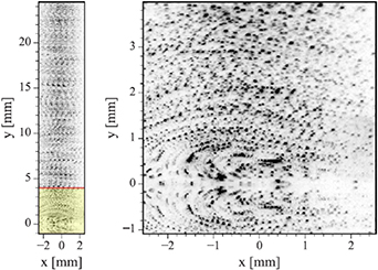
Figure 5. Detailed view of a backflow event in a ZPG TBL at  , where the right panel is an enlarged view of the region highlighted on the left panel. Reprinted from reference [135], with permission from Elsevier.
Download figure:
Standard image High-resolution imageAlthough sequences of multiple incidences of backflow events in the form of particles moving upstream for a certain duration could be observed in the aforementioned PIV studies, one of the shortcomings in those studies is related to the low seeding density and limited spatial resolution [135]. One way to overcome this deficiency is to utilize PTV instead of PIV whenever the seeding density is low, and inhomogeneous and/or non-constant flow gradients (as in the presence of backflow events) are present [144, 202]. As argued by Kähler [144], 'for wall distances below half an interrogation window dimension, the singe-pixel ensemble-correlation or PTV evaluation should always be applied', which is the case whenever wall-shear-stress fluctuations are the sole focus of an investigation. A recent work in this respect is the planar and volumetric time-resolved PTV experiment by Bross et al [201], in which near-wall extreme events in an APG TBL at  were measured. A detailed representation of their experimental setup is shown in figure 6. Based on their measurements, they proposed a conceptual model explaining the rare occurrence of backflow events, and their topology and dynamics. Their model involves a complex interaction process between low-momentum, very-large-scale structures, near-wall low-speed streaks, and tilted longitudinal and spanwise vortices located in the near-wall region. Backflow events are then observed when a low-speed, large-scale motion coincides with a low-speed streak and its meandering tilts streamwise vortices. Note that this is compatible with the mechanisms reported by Lenaers et al [37]. Three-dimensional separation in an APG TBL was characterized experimentally through planar and tomographic PIV by Elyasi and Ghaemi [203]. Their results reveal that, in this configuration, forward and backward flows have approximately equivalent strength (a conclusion confirming the numerical results by Vinuesa et al [187]) and the fact that the conditional average of the flow at the instant of separation forms a saddle-point structure with streamlines converging in the spanwise direction, as shown in figure 7. They also performed POD and concluded that the spatial modes show focus, node and saddle-point structures as well. Elyasi and Ghaemi [203] used the average of the coefficients of the dominant POD modes during the separation events to develop a reduced-order model (ROM). Based on the ROM, it can be stated that the instantaneous three-dimensional separation is a saddle-point structure interacting with focus-type structures.
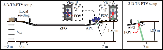
Figure 6. Schematic representation of the experimental setup for 2D and 3D PTV by Bross et al [201]. Reproduced with permission from [201]. © 2019 Cambridge University Press.
Download figure:
Standard image High-resolution image
Figure 7. Conditional average of the fluctuating flow field around a separated region in an APG TBL obtained through tomographic PIV. (Blue), (green) and (yellow) show regions of positive, zero and negative velocity, respectively; the figure also shows convergence of streamlines in the spanwise direction. Reproduced with permission from [203]. © 2018 Cambridge University Press.
Download figure:
Standard image High-resolution imageAnother type of APG TBL, in this case the one developing on the suction side of a NACA4418 wing section at Rec = 750 000, was studied with wall-parallel PIV by Ma et al [204]. In particular, the wall-shear-stress vector in the separated area was measured by means of the FOV denoted as FOV2 in figure 8 (left), which shows the experimental setup. This setup allowed Ma et al [204] to characterize the near-wall streamlines, which exhibited a saddle point around the center of the wing in the spanwise direction, flanked by two counter-rotating foci, the formation process of which is shown in figure 8 (right). It is important to note that these structures could not be visualized in the instantaneous fields and low-pass filtering had to be used in order to observe them. The authors reported that the foci are formed by an influx of momentum from the backflow region and their alternating processes of production and destruction lead to the intermittency of the separation line. This experimental campaign provided a highly detailed characterization of the complex mechanisms present in the near-wall region of APG TBLs.
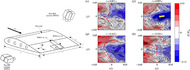
Figure 8. (Left) Representation of the experimental setup employed by Ma et al [204], showing the FOVs and the positions of the cameras. (Right) Dynamic representation illustrating the influx of momentum originating at the reverse-flow region. Reproduced with permission from [204]. © The Author(s), 2020. Published by Cambridge University Press.
Download figure:
Standard image High-resolution image4.3. MPS3 measurements of extreme events
Micro pillars were used by Brücker [177] to measure near-wall backflow events and critical points (i.e. points of zero wall-shear stress) in a ZPG TBL at  . This could be considered as the first experimental confirmation of the existence of backflow events in wall-bounded turbulence and figure 9 shows the process to analyze the original micro-pillar photograph in order to obtain the topology of the corresponding critical point. MPS3 sensors were also employed by Liu et al [205] to measure both wall-normal velocity spikes and backflow events in a turbulent channel at
  and 1300. They confirmed an inner-scaled diameter of around 20 for the backflow regions and reported that negative wall-normal velocity spikes occur together with strong streamwise wall-shear stress, whereas strong spanwise motions are associated with large positive spikes. They also argue that it would be important to take into account the length-integrating effect of the pillars, which may, however, lead to errors in determining higher-order statistics. One possible alternative could be to use shorter pillars, although these would produce a lower deflection which would require a smaller FOV. In this case, it could be possible to modify the flexibility of the pillar, with the aim of increasing the deflection for the same load. Nevertheless, an increased flexibility might produce additional measurement artifacts and limit the use of the MPS3 sensor at higher
  , which requires a larger frequency bandwidth.

Figure 9. (Left) Original micro-pillar image, (middle) vectorized version of the image and (right) visualization of the corresponding saddle–node pair. Reprinted from [177], with the permission of AIP Publishing.
Download figure:
Standard image High-resolution image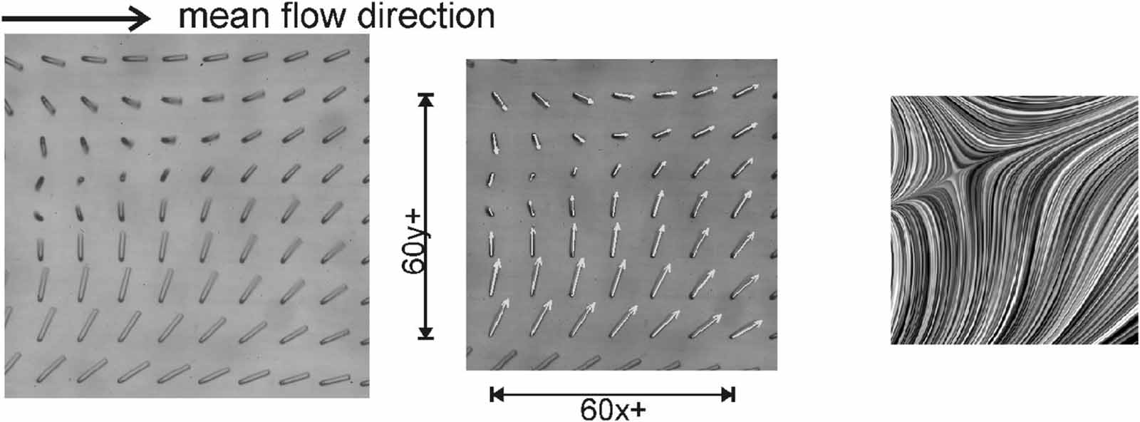
5. Summary and outlook
In this article we provide a review of some of the most widely used methods to measure the wall-shear stress and its fluctuations in wall-bounded turbulence. A number of techniques for mean wall-shear-stress measurements rely on the mean velocity profile and are based for instance on measurements in the viscous sublayer or the Clauser chart (with prescribed log-law constants). Other methods exploit the connection between the wall-shear stress and the heat-transfer rate to the fluid (for instance, surface hot-film and wall-mounted hot-wire probes), or the relation between flow velocity, pressure and friction (including streamwise pressure gradient in internal flows, Preston tubes and Stanton tubes). It is desirable to obtain direct measurements of the mean wall-shear stress and one of the devices allowing this type of measurement is the floating element. Despite its limitations, a new design [99] allows one to obtain accurate measurements of the wall-shear stress both in smooth and solid walls. When it comes to fluctuating wall-shear-stress measurements, MEMS-based floating element sensors [206–209] have, despite having existed for nearly as long as their thermal anemometry counterparts, still not been used as widely as their macro-scale counterparts. A widely used method for direct measurement of the mean wall-shear stress is oil-film interferometry (OFI), which is still the most accurate way to measure the mean wall-shear stress, with error levels of around 1% [108, 110].
A number of advanced optical techniques have become progressively more widely used to measure the wall-shear-stress fluctuations over the past years. These include laser Doppler anemometry (LDA), particle image and tracking velocimetry (PTV and PIV), molecular tagging velocimetry (MTV) and micro-pillar shear-stress sensors (MPS3). Thermal-anemometry-based techniques such as hot-film and hot-wire probes have, despite their superior frequency response (in case of hot-wire probes) and above all quick and easy implementation and data reduction, increasingly been superseded by other techniques when it comes to fluctuating wall-shear-stress measurements. Nonetheless, they remain widely used—fully acknowledging their limitations—e.g. as sensors for the detection of flow features occurring farther away from the wall in flow-control studies or for studies limited to large-scale features of the flow. Mainly, the PIV and MPS3 methods have helped to shed some light on the characteristics and dynamic behavior of near-wall extreme events, including regions of reverse flow (backflow events) and critical points (points of zero wall-shear stress). Comprehensive PIV campaigns have been carried out in ZPG TBLs up to  [135, 199], reflecting the complexity of backflow events and the challenges associated with their measurement. For instance, differences regarding the size and convection velocity of backflow regions have been found between experimental [135] and numerical data [186, 187]. PTV and PIV have been employed to characterize the dynamics of the near-wall region in APG TBLs, including the interaction between large-scale and backflow events [201] and the characteristics of the wall-shear-stress vector [203]. Brücker [177] and Liu et al [205] employed MPS3 to measure and study backflow events and critical points in wall-bounded turbulence. They confirmed some of the conclusions previously reported in DNS [37], but they indicated that there are some challenges related to the length-integrating effect of the pillars, particularly at progressively higher
  . Many of the advances in PIV and PTV, and their application in high-Reynolds-number wall-bounded flows, will also keep pushing the limits of laser-optical velocimetry, one of these directions being the Shake-the-Box (STB) approach [151]. In particular, MTV, thanks to the recent development in improved spatial resolution and the applicability of green lasers (with their commercial availability in most laboratories) with high frequencies and high powers (which are predominantly used in experimental fluid dynamics laboratories), is expected to be one of the most promising techniques when it comes to fluctuating wall-shear-stress measurements. The aforementioned techniques have been summarized in table 1 including their main characteristics, i.e. whether they are direct/indirect, require a calibration and are able to measure the fluctuating component, and some of their main limitations or features.
Table 1. Summary of wall-shear stress measurement techniques discussed in the present review with their main characteristics, i.e. whether they are direct/indirect, require a calibration and are able to measure the fluctuating component. We also include additional comments from each technique and the sections in which they are discussed. Note that all measurement techniques require certain calibrations, but that the one referred to here implies that the physical quantity measured is calibrated against a known wall-shear stress.
| Measurement | Direct | Calibration | Time- | ||
|---|---|---|---|---|---|
| technique | method? | required? | resolved? | Comments | Section |
| Preston tube |  |
a) presumes known inner layer profile | 2.3 | ||
| Stanton tube |  |
b) presumes known sublayer profile | 2.3 | ||
| Surface fence |  |
[MEMS  ] ] |
c) bi-directional, d) MEMS versions provide temporal information | 2.3 | |
| Floating element |  |
[MEMS  ] ] |
c), d) | 2.4 | |
| OFI |  |
c), e) provides shear stress angle, f)  calibration crucial calibration crucial |
2.5 | ||
| HWA/HFA |  |
 |
g) based on equation (1), h) limited to  |
2.2/3.1 | |
| LDA |  |
g) | 3.2 | ||
| LDV profile sensor |  |
g), i) improved spatial resolution compared to LDA | 3.2 | ||
| PIV/PTV |  |
g) | 3.3 | ||
| MTV |  |
j) improved spatial resolution compared to PIV/PTV | 3.4 | ||
| MPS3 |  |
 |
g), k) provides instantaneous 2D field information | 3.5 |
In conclusion, despite the significant progress experienced in the area of high-quality measurements of near-wall events in wall-bounded turbulence, further development on the accuracy and robustness of these methods is needed. In particular, backflow events play a progressively more important role as the flow approaches mean separation, due to the increased wall-normal convection and reduced near-wall mean velocity induced by the APG. We argue that a very important challenge to be addressed in the future is to accurately measure backflow events under dynamically changing flow conditions, such as for instance in the context of pitching airfoils [179]. The benefit is twofold: from a (fluid-)physical point of view, improved knowledge of the dynamic behavior of these events in such conditions would pave the way towards a deeper understanding of the mechanisms leading to flow separation, an essential aspect to control in order to improve the aerodynamic performance of aircraft and generally increase the efficiency of a wide range of applications. When it comes to measurement-technique developments, however, these backflow events constitute a clear challenge and an incentive on which the temporal and spatial resolution, dynamic range, and multi-directional capabilities of a measurement technique can be tested. This is partially the reason why there has been renewed interest in these events as in the detailed DNS study by Lenaers et al [37].
Acknowledgment
The authors acknowledge the financial support from the Swedish Research Council (VR).
Footnotes
- 1
It is worth noting that the Reynolds-number-dependent increase of the inner peak of the streamwise variance profile has recently also been observed in the Superpipe [27].
- 2
It should, however, be noted that special optical arrangements of LDV systems are found in the literature that achieved measurement volumes an order of magnitude smaller than those of conventional systems; see e.g. reference [128]. This arrangement has also provided one of the most cited turbulence measurements in a turbulent boundary layer, since it provided one of the first turbulence statistics that exhibited the correct Reynolds-number trend, which otherwise would be obscured by insufficient spatial resolution [20].