


Abstract
This paper presents a non-intrusive measurement technique for the simultaneous assessment of the three-dimensional (3D) velocity and temperature fields in thermal convection. The technique is based on the combination of tomographic particle image velocimetry and particle image thermometry. Thermochromic liquid crystal particles serve simultaneously as both flow tracers and thermometers. The velocity fields were measured in a volume of 62 500 cm3 and the temperature fields in a subvolume of 20 000 cm3. Turbulent Rayleigh–Bénard convection in a water-glycol mixture at  and
and  was used as a model system to measure the instantaneous 3D velocity and temperature fields at the same time. Uncertainties of
  mm s−1 for the velocity and
  K for the temperature measurement were estimated corresponding to dynamic ranges of 24 and 21 levels, respectively. Correlating the measured temperature and velocity fields, it is shown that the obtained large-scale structure reflects a region of warm rising fluid which is well-known from the literature.
Export citation and abstract BibTeX RIS
1. Introduction
Turbulent thermal convection occurs frequently in nature, e.g. in atmospheric movement, and many technical applications such as ventilation systems and heat exchangers. The most prominent thermal convection problem is known as Rayleigh–Bénard convection (RBC), which has been studied extensively in the past, see e.g. [1–3] and two comprehensive review articles [4, 5]. For many years, research on RBC has focused on the heat transport from the lower heated plate through the fluid layer to the upper cooled plate. In turbulent RBC this heat transfer is associated with the turbulent heat transport which is a correlation of temperature and velocity fluctuations [4].
A well-established technique to measure the velocity field is particle image velocimetry (PIV) [6], which is based on two images recorded at two separated time instants in order to determine the velocity field within the measurement plane. For example, large-scale PIV was applied in RBC to investigate the boundary layer structure in an air experiment with a height of 9 m and varying diameter [7]. With the introduction of tomographic particle image velocimetry (Tomo-PIV), the non-intrusive acquisition of all three velocity components (3C) of the velocity field in a measurement volume (3D), i.e. 3D-3C-Tomo-PIV, for dense particle distributions became possible [8, 9]. Using this method, the 3D velocity fields in a measurement volume as large as 840 × 500 × 240 mm3 were determined in [10] to study the flow structures in a mixed convection sample. The analysis of the obtained mean velocity field revealed a large-scale convection roll with a core line and a wavy shape.
In contrast to the well-established velocity field measurements, most temperature measurements are performed with sensors installed in or close to the wall. However, there are also non-intrusive methods to measure the temperature fields in planar fields of view. A well-known example is the so-called laser induced fluorescence (LIF) [11, 12], which uses fluorescent dye particles excited by an appropriate light source. Their temperature-dependent emission spectrum is recorded and analysed. Often, two dye types with non-overlapping emission spectra are used to reduce uncertainties. Typically, LIF can be applied in case of temperature fields with an inherent temperature difference of more than 10 K [13]—usually more than 40 K [14]. Non-intrusive temperature measurements of temperature fields covering values differing by less than 10 K are investigated with particle image thermometry (PIT) [15]. Thermochromic liquid crystal (TLC) particles [16, 17] are illuminated by white light acting as fluid thermometers are used due to their temperature-dependent wavelength reflection.
Furthermore, simultaneous measurements of velocity and temperature fields are described in [18] by Liot et al who used a spherical flow tracer equipped with several temperature sensors and a diameter of 2.1 cm. In a convection sample filled with water, the density of their so-called smart particle was adjusted to achieve neutral buoyancy. Exploiting advection, the particle was used to measure the temperature at different locations of the sample, while its movement was recorded as a two-dimensional (2D) projection by a CCD camera. Thus, the projected 2D velocities and associated temperatures in the entire volume could be determined but only at one point at a time.
Another non-instrusive measurement technique allowing for the simultaneous acquisition of temperature and velocity fields is the combination of LIF and PIV. It was applied in a natural convection experiment to measure the two fields in the same 2D plane [19] and in a microfluid experiment in [13] to systematically study the processing algorithms.
However, even more relevant for the present work is the combination of PIT and PIV used in [20–22] to measure the temperature and two components of the velocity fields in planes of a natural convection sample. The extension to the measurement of all three components of the velocity field simultaneous to the temperature field in planes was realized in an experiment with water by combining PIT with stereo PIV [23]. Fujisawa et al investigated the convection patterns by means of POD analysis and identified a large-scale motion. Using RBC in water as a model system, an extension of the PIV–PIT technique which employs artificial neural networks for the calibration procedure is presented in [24]. In the latter study an uncertainty for the temperature measurement on par with a linear interpolation approach is reported and the possibility for uncertainty reduction using a multi-variable approach is shown. The reader is further referred to the reviews [15, 16, 25] for more details of TLC particles and their usage in PIV/PIT.
Finally, astigmatism particle tracking velocimetry (APTV) is combined with TLC particles in [26] to measure the 3D Lagrangian velocity field in combination with the 3D temperature field to study the flow in a warm cooling water droplet. APTV applications usually feature two resolved velocity components and a rather uncertain third one. In [26] the temperature changes along several trajectories are visualized by means of APTV and PIT. A combination of APTV and PIT is also used in [27] to measure the flow in a heated micro-channel. The authors focused on determining the uncertainty of the measurement technique by applying highly accurate experimental temperature monitoring of the boundary conditions and comparing the derived fields to additional numerical simulations. For a temperature measurement range of 10 ∘C an uncertainty below 1 ∘C is reported.
In the following, a measurement technique for the acquisition of 3D large-scale temperature and velocity fields will be introduced and employed to investigate the flow in RBC taking the typically small temperature differences in thermal convection into account. TLC particles have been used as flow tracers in an RBC sample filled with a water-glycol mixture and illuminated by a white light LED array. The particle position and velocity have been deduced from the intensity maps of the Tomo-PIV and used for the PIT to measure the temperature within the volume. This allows for the acquisition of dense temperature and velocity fields.
2. Experimental setup
A sketch of the rectangular RBC sample with a volume of 62 500 cm3 filled with a water-glycol mixture used in the experiment is shown in figure 1. The top and bottom of the sample were embedded in a 10 cm styrodur insulation mantle (a). The temperature of the cooling plate (b) was controlled by a water circuit, whereas the temperature at the heated plate (f) was maintained using a resistive heating device. Both temperatures were kept constant at ±0.05 K. The two mentioned temperature control systems were embedded in anodized black aluminum plates, (c) and (e), enclosing the sample. The side walls (d) were made of 10 mm thick glass providing high optical accessibility. The set-up was supported by polyoxymethylen (POM) spacers, (g), installed within the insulation. They were leveled to connect the heating element and the ground plate. Moreover, the spacers exhibited a high stability and were mounted on a hardened aluminum ground plate (h), thus maintaining a long-term alignment of the set-up to the horizontal within 0.01∘. In figure 1 the characteristic length of the sample corresponds to the height  .
.
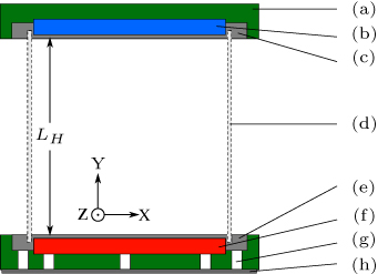
Figure 1. Schematic of the cubic RBC sample in Z-direction. (a) marks the insulation layer, (b) and (f) indicate the cooling and heating elements and (c) and (e) mark the anodized aluminum plates enclosing the sample. The glass cube (d), the POM spacers (g), and the hardened aluminum ground plate (h) are labeled. The characteristic length of the sample is indicated by  .
.
Download figure:
Standard image High-resolution imageWith the temperatures of the heating plate and the cooling plate,  and
and  , the average sample temperature amounts to
  and the temperature difference is
  . RBC is characterized by two dimensionless numbers, the Prandtl number
and the Rayleigh number
with the kinematic viscosity ν, the isobaric thermal expansion coefficient β, the dynamic viscosity η, the thermal conductivity λ, the thermal diffusivity α, the gravitational acceleration g and sample height  .
.
The measurement volume was illuminated by a high-power white-light LED array consisting of 15 × 15 LEDs of the type Osram Platinum Dragon LW W5SNA with a broad wavelength distribution covering the entire visible light spectrum. The LED array was triggered by a high-current power supply that provided defined light pulses of sufficiently high intensity to record the reflected color of the TLC particles. Focusing optics were positioned in front of the LEDs to reduce the divergence of the light and, thus, to generate a homogeneous intensity distribution within the measurement volume with light intensity fluctuations below 10%. It must be noted that the array was designed for low flow velocity measurements with an applicable illumination duration between 100 µs and 1200 µs. For more details on the LED array, refer to [3].
A sketch of the employed camera setup is presented in figure 2. The side view shows the aluminum heating and cooling plates, indicated by (a) and (b). Four black-and-white (b/w) PCO1600 CCD cameras, (c) to (f), with a resolution of 1600 × 1200 pixels were used to monitor the convection sample from different angles. With these four cameras the velocity fields were measured in a sample with a height of 500 mm, a width of 500 mm and a depth of 250 mm. A PCO-Pixelfly color CCD camera (g) monitored a subvolume close to the cooling plate. Each camera was equipped with 21 mm Nikon lenses and tilted in accordance with the Scheimpflug condition. The sample was illuminated by the LED array (h) shown in the top view and is highlighted in yellow. The subvolume for the simultaneous temperature and velocity measurements close to the cooling plate is indicated by the striped area in yellow.

Figure 2. Sketch of the experimental setup for the simultaneous 3D velocity and temperature field measurements. The velocity field measurement volume in the front half of the sample is highlighted in yellow and the temperature measurement volume is indicated by the yellow area with stripes. (c) to (g) mark the cameras and their lines of sight are shown as dashed lines. In the side view, (a) and (b) present the heating and cooling plate. In the top view the light source is indicated by (i).
Download figure:
Standard image High-resolution imageIn the present study, TLC particles (Hallcrest, R18C6) were used. Typically, those chiral nematic crystals have a relaxation time between 1 and 10 ms [28–31] and are thus suitable for the low flow velocities considered in the present study. Therefore, in order to use TLC particles in combined Tomo-PIV and PIT, three major requirements were identified:
- A homogeneous TLC particle size distribution.
- Neutral buoyancy in the fluid.
- Recording as much color information as possible.
In terms of the first requirement, a homogeneous distribution of the sizes of tracer particles is necessary to guarantee similar images. In the present study, the custom-manufactured encapsulated TLC particles were delivered with sizes varying between 1 µm and 2000 µm. In general, large particles scatter more light and are consequently preferred over smaller ones. Yet, the distribution of sizes showed that larger particles are rarer. Thus, in order to provide sufficiently bright particle images, a minimum size of 40 µm was estimated. To find a compromise between the availability of particles with a certain size and the application of particles as large as possible, particles with a size between 100 µm and 110 µm were selected in a multiple filtering process using sieves with different mesh openings.
Moreover, the TLC particles have to be buoyancy neutral on average. This was achieved by performing the measurements in a water-glycol mixture. For a mass mixing ratio of  , about 90% of the particles showed neutral buoyancy, the others were discarded. This behavior indicates a non-constant ratio of the TLC core and hull making this selection step even more important since the reflective characteristic can be affected.
The last requirement was to record as much color information as possible. Typically, TLC particles show the most pronounced color play in the backwards-scattering direction [16]. Therefore, the PCO-Pixelfly color CCD camera with integrated Bayer filter and a resolution of 1392 × 1024 pixels was installed accordingly. In addition, the specified color play of custom-manufactured TLC particles had to be selected with respect to the investigated temperature range.
The Bayer filter of the color camera reduces the light sensitivity by more than a factor of four with respect to a comparable b/w camera. To ensure an equal signal quality between the four cameras used for PIV and the color camera used for PIT, a smaller volume of ≈20 000 cm3, presented by the striped area in figure 2, was monitored in case of the color camera. A sufficient signal-to-noise ratio of 4 for this subvolume was achieved. Moreover, the probability of imaging multiple TLC particles on the same pixels of the camera is about three times smaller in the reduced PIT subvolume.
The considered turbulent RBC in the sample sketched in figure 2 was characterized by the temperature of the heating plate,  C, and the temperature of the cooling plate,
  C. This resulted in a mean temperature of
  C and a temperature difference of
  .
.
For the employed water-glycol mixture the characteristic numbers were  and
and  . The particle images were recorded with a time separation of Δt = 150 ms, i.e. a recording frequency of f = 6.6 Hz resulting in an average particle displacement of 6 pixels per timestep. Thousand images were recorded and used afterwards for the statistical post-processing. The interpretation of the amount of images in terms of physical flow properties of the RBC can be found in the results section 4.1.
3. Combined tomo-PIV–PIT
In the following the combination of Tomo-PIV and PIT to allow volumetric temperature and velocity field measurements will be described. The first section 3.1 provides an overview of the combined method. In section 3.2 the intensity filter used to reconstruct the particle positions in 3D space is described. Finally, section 3.3 illustrates how the colors are calculated from the acquired images and how they are used for the color-temperature calibration.
3.1. Method overview
The workflow of the combined Tomo-PIV–PIT is illustrated in figure 3. Four b/w cameras monitored the convection sample from different viewing angles. They provided four image pairs of the TLC particles at two time instants, t and t + Δt. The mapping functions from 3D ( ) to 2D (
 ) space were obtained performing a volume self-calibration [32] with a calibration plate. This yielded the fitted 38 parameters for a Soloff polynomial function F [33] describing the translation
  for each camera involved. Using an in-house Tomo-PIV code, which is described in detail in [10, 34], the simultaneous algebraic reconstruction technique (SMART) [35] was employed to determine the intensity distribution in 3D space, which was afterwards subdivided into interrogation volumes. Subsequently, a 3D cross-correlation between the two time steps is conducted in order to calculate the average displacement within each volume. By combining the time separation Δt with the displacement, the velocity field is obtained.

Figure 3. Illustration of the combined Tomo-PIV-PIT workflow based on data acquisition with five cameras. On the Tomo-PIV side of the chain, the intensity distribution is calculated and divided into interrogation volumes. A 3D cross-correlation provides the displacement, which allows to calculate the velocity field. A temperature-color calibration is performed to transform the color fields into temperature fields. The 3D temperature fields are determined by combining the 3D intensity distribution and the 2D temperature fields. The 3D temperature fields are combined with the velocity fields to provide the combined velocity and temperature fields.
Download figure:
Standard image High-resolution imageIn addition, a color CCD camera recorded the color information of the TLC particles used to determine the lightness and the hue maps, as explained in more detail in section 3.3. To relate the two-dimensional images recorded by the color camera to the desired 3D fields in the measurement volume, the volume self-calibration with the four b/w cameras was repeated after adding the color camera to obtain the required translation function for it. The lightness of the pixels on the color images serves for the particle detection, while the hue maps are used for the color-temperature calibration resulting in the temperature maps.
The calibration was performed by setting the temperatures of the heating and cooling plate to the same temperature value  . After an average settling time of eight hours, 10 000 color images of the TLC particles were recorded. Then, the hue values H were determined at all points in the measurement volume. Subsequently,
  was changed to determine the corresponding hue values. Since H is affected by the viewing angle of the camera, it was necessary to divide the color image into finite subregions. The calibration curve translating H into T was obtained for each subregion, see section 3.3.
The positions of the TLC particles were determined based on the 3D intensity maps provided by Tomo-PIV, see figure 3 (top right), which considers only the four b/w cameras. Afterwards, the temperature values obtained by PIT were assigned to the 3D positions defining 3D PIT, see figure 3 (center). For this assignment the translation function  of the color camera was used. Ambiguities can occur when a particle on the camera is assigned to multiple 3D positions resulting from the same line of sight. Assuming that the particle closest to the camera covers the more distant ones, the ambiguity was resolved by assigning the temperature value only to the 3D position closest to the camera.
3.2. Determining the 3D positions
The 3D particle positions were obtained from the intensity maps calculated in the SMART reconstruction during the Tomo-PIV evaluation. Due to a blurring applied during the reconstruction the particles were represented as a Gaussian distribution. Thus, a Gaussian curve fitting was used for the position recovery of the particles. This fitting employs the ROOT Toolkit [36] to recover the 3D position and to save computational time.
In brief, the workflow of the particle position reconstruction process can be summarized as follows: The positions were reconstructed by taking the highest intensity value found in an intensity map into account first. At the location of this value an initial estimation of the particle position uses one 1D Gaussian curve fit for each spatial direction. These results were then used as starting values for a subsequent 3D Gaussian fit improving the accuracy. Moreover, this procedure proved to be more stable than a direct 3D Gaussian curve fit to the data. The determined central value of the fit represents the position of the particle in 3D space. Afterwards, all intensities considered for the fit were subtracted from the intensity map. The procedure was reiterated to reconstruct as many particles as possible until the noise threshold of 75 intensity units was reached where no further particles could be identified.
Due to the high computational effort of the process—nine hours on average per map using a single core—a parallel implementation was employed. The curve fitting was performed using 20 threads in parallel on an Intel Xeon E5-2680V2 with Hyper-Threading enabled reducing the real time to less than two hours per map. Exclusive subvolumes were assigned to the individual processes in order to avoid ambiguities which might be introduced by removing already used intensities.
3.3. Color-temperature calibration
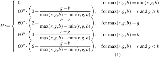
A color camera recorded the scattered light of the TLC particles and thus the contained temperature information. This data is typically acquired in the common RGB color space, yet it is known that other representations are more suitable for the required color-temperature calibration [16]. The two most common color spaces are hue-saturation-lightness (HSL) and hue-saturation-value (HSV). In the present study, a transformation of the color space from RBG to HSL was applied to calculate the temperature from the color information of the TLC particles. Since H represents the raw color, it is only sensitive to the color composition and therefore used for the color-temperature calibration. It is commonly calculated as follows:
The saturation S indicates the colorfulness, i.e. S = 0 describes grayscale and S = 1 the pure color. The lightness, L, is usually considered as a combined brightness of the color given by
For completeness, the parameter V represents the raw brightness given by  . Both values, L and V, have in common that 0 means black and 1 represents the bright color. The HSL color space was chosen for the present study and L was used for particle detection since slightly more particles were detected as compared to V.
A sketch of the employed processing chain for the color-temperature calibration is presented in figure 4. Five major steps are performed to determine the necessary dependence of the color on the temperature:
- Setting the calibration temperature
 .
. - Transforming the color space from red-green-blue (RGB) to HSL.
- Determining the central hue values in interrogation windows using a Gaussian curve fit.
- Reiterating for multiple calibration temperatures.
- Employing the H(T)-value pairs in a curve fit to estimate the color-temperature calibration curves.

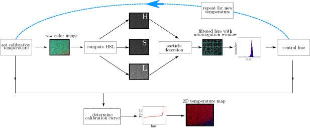
Figure 4. Sketch of the processing chain for the color-temperature calibration.
Download figure:
Standard image High-resolution imageTo avoid scaling issues, H and L are given in units of 212 = 4096 in accordance with the maximum bit depth of the color camera. Using the information delivered by the calibration images, only the TLC particles with a certain quality i.e. brightness  were taken into account and the 2D hue maps were determined based on the 2D color images. Here, only the pixel coordinate defines the viewing angle which is presented as a 2D sketch of the imaging process in figure 5. The light source illuminates the particles from the left-hand side. Two lines of sight each crossing two particles are indicated. On one line of sight (red) a constant angle α with respect to the incident light is present, although the two indicated particles are positioned at different depth. Similarly, for the other line of sight (purple) a constant angle β is present which is different from the former one and again two particles at different depth are shown. Thus, it is not necessary to consider the depth-wise (and the parallel directions) in the volume separately and it is sufficient to employ small interrogation windows with a size of 100 × 100 pixels on the 2D hue maps to compensate for the viewing angle-dependent color reflection of the TLC particles.
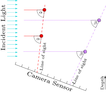
Figure 5. 2D sketch of the imaging process with the light source illuminating the particles from the left hand side. Two lines of sight for two pixel each crossing two particles are indicated. Two angles with respect to the incident light on two lines of sight are presented. Two particles per line of sight are indicated at different depth.
Download figure:
Standard image High-resolution imageWithin each of these windows, a 1D Gaussian curve fit was performed for the reduced hue-value distribution. The deduced center value,  , was stored together with the corresponding calibration temperature for the desired temperature range to reach a sufficient number of values pairs
  . This allowed to determine the functional dependence T(H) using a curve fit with the following function to estimate the parameters pi
:
. This allowed to determine the functional dependence T(H) using a curve fit with the following function to estimate the parameters pi
:
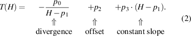
While parameter p0 is a scaling parameter, p1 shifts the hue values and causes a divergence in the analytical function at the position of the blue stop of the TLC tracer particles. p2 levels the temperature curve in accordance with the red start of the particles and parameter p3 reflects the linear dependence of temperature and hue value. The obtained functions were used to translate the hue values into temperatures. For the presented measurement, this calibration routine results in 14 × 11 = 154 calibration curves.
4. Results
The velocity fields measured with Tomo-PIV are discussed in the first section, 4.1, of this chapter. Afterwards, the temperature fields obtained from Tomo-PIT are discussed in section 4.2. Then, in section 4.3 the velocity and temperature fields measured with the combined Tomo-PIV-PIT approach are presented. This is followed by a more detailed analysis of temperature-velocity correlations and integral quantities in section 4.4. In the last section, 4.5, the uncertainty evaluation is presented and discussed.
4.1. 3D velocity field measurement
For the Tomo-PIV a particle image density of 0.035 particles per pixel (ppp) on the four camera images was realized. From the latter, 1000 instantaneous velocity fields were determined using the Tomo-PIV processing path of the evaluation workflow, see figure 3. The number of fields was chosen as a compromise between suppression of turbulent fluctuations and high statistics. The particles on the camera images were identified using an image pre-processing approach consisting of a minimum image subtraction, image normalization with 101 × 101 pixel kernel, high-pass filter with 31 × 31 pixel kernel, thresholding at 600 intensity units and a three-point Gaussian fit with 3 × 3 pixel kernel. The obtained particle distributions were then used for the intensity reconstruction, see figure 3 (top right), employing 1000 × 1000 × 500 voxels for 500 × 500 × 250 mm3 in physical space. Afterwards, a cross-correlation algorithm with grid refinement was applied to determine the velocity fields. The interrogation windows started with a size of  and were refined to
  with an additional overlap of 50%. For the resulting velocity fields, a basic outlier detection was performed flagging only 0.9 percent of the vectors as invalid. Those were replaced using the surrounding 26 vectors, and the first reiteration of the outlier detection did not reveal any remaining invalid vectors.
In order to determine the dominant behavior of the investigated flow, the resulting velocity fields were statistically evaluated by means of temporal averaging  . Figure 6 shows the time-averaged velocity field using three-component vectors. Color-coding and vector scaling reflect the velocity magnitude,
  . Increased velocities between 4 and 6 mm s−1 along a circular path within the X-Y planes can be seen. There is an upstream region at the left side of the sample (X ≈ 50 mm) and a downstream region at the right side (X ≈ 450 mm). In RBC, this structure is typically termed large-scale circulation (LSC). Its normal vector points in Z-direction but is not exactly aligned. An important characteristic of the LSC is its highest velocity magnitude of the time-averaged velocity field:

Figure 6. Time-averaged velocity field at  and
and  . The velocity is represented by three-component vectors and the color-coding corresponds to the velocity magnitude.
Download figure:
Standard image High-resolution imageMoreover,  can be used to determine statistical convergence by expressing the measurement duration
  by means of a simplified circulation period of the LSC,
  . In order to do so, a circular flow structure covering the sample is assumed and with a length along the circular path amounting to
  . Here, it is compared to the distance s1000 which the flow covers within the 1000 evaluated timesteps:
Thus, the low-frequency oscillations of the LSC remain present, whereas the high-frequency turbulent fluctuations are suppressed.
The fundamental flow properties are studied by means of a histogram plot of the velocity magnitude obtained from the 1000 instantaneous fields presented in figure 7. The absolute number of values per bin is shown for a bin width of  mm s−1. The complete distribution over the entire velocity range shown in blue in figure 7 reflects a maximum value of 18 mm s−1. In the upper right corner, a close-up view of the distribution between 13.5 and 17.5 mm s−1 is plotted in green. Since absolute velocity values larger than
  mm s−1, indicated by the red line in figure 7, are rather rare, the latter velocity was considered as the maximum velocity in the instantaneous fields and was used to estimate the dynamic range of the measurements. From the smoothness of the distribution it is concluded that no peak locking occurs indicates the high quality of the Tomo-PIV.

Figure 7. Velocity magnitude of all vectors from the 1000 instantaneous velocity fields. In the upper right corner, a close-up view of the distribution between 13.5 and 17.5 mm s−1 is shown. The end of the distribution is highlighted by a red line red.
Download figure:
Standard image High-resolution image4.2. Temperature measurement
Figure 8 shows an example of an instantaneous color image recorded by the PCO Pixelfly color camera reflecting a particle image density of 0.025 ppp. It must be noted that the color scale provided by TLC particles is counter-intuitive as red reflects the lowest and blue the highest temperature values. The color play of the TLC particles is illustrated by green crystals on the left-hand side and red particles on the right-hand side—which can generally be attributed to the dependence on the viewing angle [16] and illustrates the necessity for the smaller calibration windows to compensate for this reflection characteristic of the TLC particles, see section 3.3.
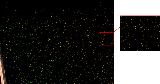
Figure 8. Instantaneous color image taken by the PCO Pixelfly color camera. The color play of the TLC particles reveals dominantly green TLC particles on the left side and red particles on the right side. A close up view is presented on the right hand side.
Download figure:
Standard image High-resolution imageIn order to prove the applicability of the TLC particles to the temperature measurements, the dependence of the hue values on the temperature was investigated. First, the TLC particles had to be identified on the color-camera images. After the color-space transformation, a noise level of up to L ≈ 300 was reported. Here, the TLC particles were separated from the noise using a threshold at L = 800. Afterwards, the hue value distribution of the identified particles was studied by means of histogram plots presented in blue in figure 9 for four calibration temperatures. Ten thousand color images were taken into account to determine the distribution for each calibration point. In addition, the approximate regions for red, blue and green to violet are shown in the background. In general, an increase in temperature resulted in a shift of the distribution from red (18 ∘C, cold) towards blue (20 ∘C, warm). Further, it can be seen that there are no values for the violet area. This was to be expected based on with the typical behavior of the TLC particles [16] and shows that the implemented Bayer filter and the hue value calculation work as assumed. The distributions at 20 ∘C and 22 ∘C were quite similar revealing that a change in the temperature between 20 ∘C and 22 ∘C does not affect H. Thus, it can be concluded that the particles' temperature resolution decreases as soon as the temperature exceeds 20 ∘C. Further, the 19 ∘C calibration point showed a large concentration of values in the green region and an additional, however, about 3.5 times smaller, agglomeration in the blue region. This proved the necessity for the individual calibration windows and the associated calibration functions to account for this non-uniform behavior.

Figure 9. Distribution of the hue values for calibration temperatures of 18 ∘C, 19 ∘C, 20 ∘C and 22 ∘C. In addition, the approximate areas for red, blue and green are shown in the background.
Download figure:
Standard image High-resolution imageConsequently, the calibration approach using 100 × 100 pixels interrogation windows was employed. An exemplary result at T = 20 ∘C for an interrogation window taken from the middle of the camera image is visualized in figure 10(a). The H-distribution is shown as a blue histogram. Following the procedure described in section 3.3, the corresponding 1D Gaussian curve was determined and superimposed as a black line. Based on the Gaussian curve, the center value  was determined as highlighted in red in figure 10(a). By repeating this procedure for all interrogation windows the calibration points
  were obtained.

Figure 10. (a) Distribution of hue values at 20 ∘C in a  pixels interrogation window for an anchor point of
  pixels is shown in blue. The result of a 1D Gaussian curve fit is indicated in black. The red line marks the central value
  of the Gaussian curve. (b) Result of a curve fit of
  . Black markers indicate the data points and the determined analytical function is indicated in red with the resulting parameters shown in green.
Download figure:
Standard image High-resolution imageBased on these calibration points for all interrogation windows, calibration curves were determined by fitting the Function (2). As an example, figure 10(b) shows the calibration curve obtained for the interrogation window considered in figure 10(a). The black data points represent the five calibration temperatures  with
with  representing the central hue value as discussed above. Additionally, the fitted curve is shown in red and the parameters determined from the fitting procedure are indicated in green at the bottom. Since the resulting calibration curve describes the data with negligible uncertainty, it can be used to transform hue values into temperatures. It must be noted that an ensemble of 14 × 11 = 154 curves was used for the measurements presented below.
An impression of the 2D temperature distribution is provided in figure 11, where the color coding reflects the temperature in ∘C. The image is colored in black for regions without temperature information obtained from the TLC particles. The field of view corresponds to the raw color image of figure 8. Compared to the calibration images, a less restrictive brightness threshold of L = 600 was applied for particle detection for the measurement series. The associated H was used to determine the temperature. The main part of the temperature map revealed temperatures around 18 ∘C. Nevertheless, in the lower left corner, an increased temperature of 19 ∘C to 20 ∘C was determined. This will be investigated in more detail in the following section 4.3.
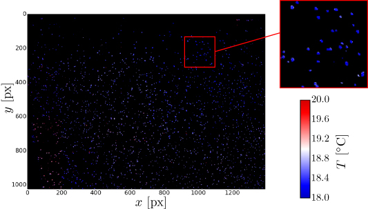
Figure 11. Instantaneous temperatures at the particle positions corresponding to the raw color image presented in figure 8. A close up view is found in the upper right corner. Color coding is chosen to reflect the temperature in ∘C.
Download figure:
Standard image High-resolution imageTo give an example of the estimation of the 3D particle position with the Gaussian curve fitting procedure described in section 3.2, the reconstructed position of a rather challenging asymmetric intensity distribution at location Y ≈ 3 mm, and Z ≈ 248 mm along X is plotted in dependency of X in figure 12. The data points are marked with blue crosses and the fitted Gaussian curve is shown in dashed green with its central value indicated in red. The intensities on the left side of the Gaussian distribution are missing, while the right side shows the expected Gaussian shape. The reason for this could be a minor misalignment of the cameras or defective/noisy pixels. When comparing the distribution with the possible position measures—mean value (447.4 mm), highest value (445.8 mm) and center of Gaussian curve fit (446.3 mm)—the results were similar. Yet, the position of the highest value suffered from a general binning and the mean value was easily offset by missing values. Only the Gaussian curve fit recovered a trustworthy position of  mm. Analogously, the coordinates
  and
and  are determined. As described before, these three results were used as starting values for a complete 3D Gaussian curve fit which resulted in a central value of
  .
.

Figure 12. Result of a 1D Gaussian curve fit at the position Y ≈ 3 mm and Z ≈ 248 mm. The data points are indicated by blue crosses and the result of the Gaussian curve fit is shown in green. The central value of the curve fitting is indicated in red.
Download figure:
Standard image High-resolution imageThe temperature value of the position which corresponds to the above-determined 3D position was then assigned to the latter using the translation functions from the volume self-calibration. The resulting 3D velocity and temperature fields will be discussed in the following section.
4.3. Simultaneous temperature and velocity field measurements
In order to unite the measured PIV and PIT data, the reconstructed 3D particle positions were combined with the 2D temperature maps from PIT using the mapping functions obtained during the volume self-calibration. On average 11 000 temperature values in 3D are obtained, while the effect of mapping multiple 3D positions with the same temperature value occurs for less than 0.1%. For such a low effect this ambiguity is solved reliably by assigning the temperature value only to the 3D position closest to the camera. A resulting instantaneous 3D velocity and temperature field is shown in figure 13. The spheres indicate the temperatures at the corresponding 3D positions in the volume using color coding. The direction of the velocity is indicated by 3C vectors, while the scaling reflects the velocity magnitude. The velocity field was determined for the entire volume, whereas the temperature measurement was limited to the upper half of the convection sample. For the sake of clarity, only every 100th vector and temperature value are shown. The structure of the LSC in this instantaneous field is similar to the structure in the time-averaged velocity field discussed in figure 6. Still, as expected for turbulent RB convection, smaller turbulent flow structures occurred throughout the measurement volume, which can also be resolved by the experimental set-up. Figure 13 shows the high upward velocities occurring within the LSC for low X values on the left and the high downward velocities for high X values on the right. The temperature values are dominantly distributed close to 18 ∘C with some increased temperature values reported for X ≈ 100 mm.

Figure 13. Exemplary instantaneous velocity and temperature field obtained during the first time step. The 3C vectors reflect the velocity using color coding with regard to the velocity magnitude. The local 3D temperature is represented by spheres whose color indicates the temperature at this point within the volume. Every 100th velocity vector as well as the temperature are shown.
Download figure:
Standard image High-resolution image4.4. Analysis of the temperature-velocity correlations
In contrast to the velocities, which were determined on a regular Eulerian grid, the temperature values were measured at the positions of the TLC particles. Thus, to be able to analyze both quantities at the same position, a 3D linear (also called tri-linear) interpolation of the temperature values measured at the particle position on the structured Eulerian grid was performed. Figure 14 reflects a resulting instantaneous velocity and temperature field in terms of scaled 3C velocity vectors which are color-coded by the temperature values at the corresponding positions. A reference vector with a velocity magnitude of 5 mm s−1 is shown at the top left. Velocity vectors at positions where no temperature value is available are visualized in gray. Outlier temperatures resulting from sporadic color fluctuations on the CCD sensor of the color camera have been removed using a simple threshold at  C and the corresponding vectors are also colored in gray. Looking at the direction of the velocity vectors, the LSC can be easily identified rotating around its center located in the middle of the measurement volume. Most of the interpolated temperatures in figure 14 show values close to the average sample temperature of 18 ∘C. For the considered fully turbulent RBC it is well-known that the temperature gradients are relatively high close to the heated/cooled plates and rather low in the bulk [18, 37]. In this respect, the measured temperatures in the bulk region are close to the mean temperature
  C. Moreover, figure 14 also reveals the existence of isolated structures by showing increased temperatures at low X values and high Y values followed by a colder structure in the upstream direction. In addition, a temperature increase to 19 ∘C with an upward flow direction on the left side of the sample (X ≈ 100 mm, Y ≈ 350 mm) is resolved. This reflects a part of the LSC which transports warm fluid from the heating plate to the cooling plate.

Figure 14. Exemplary instantaneous interpolated velocity and temperature field obtained during the first time step. 3C vectors reflect the velocity and are scaled with regard to the velocity magnitude. The color-coding represents the interpolated temperatures in the areas with the corresponding information. In the remaining volume, the vectors are kept in gray. Every 100th vector is presented. At the top left, a reference vector for a velocity of 5 mm s−1 is shown.
Download figure:
Standard image High-resolution imageIn order to quantify the dependence of upward velocity and temperature, a 2D histogram of the local temperature T and the upward velocity vy
was determined. Figure 15 shows the histogram of the instantaneous velocity and temperature field at first time step. The absolute number of pairs per bin is used as color key and the trendline is indicated in green. The velocity was divided into bins with a size of  mm s−1 and the temperature bins had a size of
  C. The dependence of T(vy
) was quantified by means of a linear curve fitting using an orthogonal distance regression in the following form:
C. The dependence of T(vy
) was quantified by means of a linear curve fitting using an orthogonal distance regression in the following form:
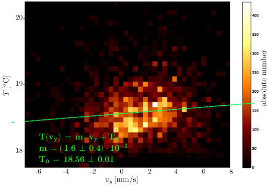
Figure 15. 2D histogram of the local temperature T and upward velocity vy
. The instantaneous velocity and temperature field at time t0 is processed as a 2D histogram with the absolute frequency per bin used as a colored key. The velocity bins have a size of  mm s−1 and the temperature bins are
  C. The result of a curve fit is shown in green in accordance with equation (3).
Download figure:
Standard image High-resolution image

Figure 15 reveals a distribution of temperature values mainly between 18 ∘C and 19 ∘C, while the velocity values range from −3 mm s−1 to 5 mm s−1. The fitted trendline parameters were  with a corresponding ordinate section
  . This reflects two important characteristics of the flow. First, a temperature distribution around
  was to be expected for RBC. In the present study, with the limited investigated subvolume the average temperature T0 was slightly above
  . Secondly, due to buoyancy, small warm structures drive the flow upwards, whereas colder ones are associated with downwards velocities [4]. For the investigated subvolume this was confirmed by a positive value for m reflecting that increased values for T yield a higher upward velocity vy
.
. Secondly, due to buoyancy, small warm structures drive the flow upwards, whereas colder ones are associated with downwards velocities [4]. For the investigated subvolume this was confirmed by a positive value for m reflecting that increased values for T yield a higher upward velocity vy
.
In the following analysis, all evaluated time steps were taken into account to make statements about the average behavior of the convective flow in the RBC sample. For this purpose, the upward velocity, the temperature and their correlation were examined based on the histograms shown in figure 16: the green histogram at the top reflects the frequency distribution of the vertical flow velocity with a bin width of  mm s−1. In blue, on the right, the corresponding temperature distribution is shown with a bin width of
  C. The correlation of the two quantities was again determined with the help of a 2D histogram, analogous to figure 15. The bin widths were chosen identically to those of the 1D histograms. The green velocity histogram shows a smooth distribution shifted towards the positive range. The shift results from the fact that the field of view of the temperature measurement was limited and thus the same limitation applies to the considered velocities. In figure 16, the blue histogram of the temperature distribution also shows a smooth curve, ranging from slightly less than 18 ∘C to approximately 20 ∘C. It is also evident that the most common value is around 18.5 ∘C, which is slightly higher than the average sample temperature of
  C. This observation is in good agreement with the flow field, as the temperature was actually measured in the region where the warm fluid flow rises from the heating plate. The 2D histogram illustrates the dominant dependence of the fluid temperature on the upward velocity. The presented distribution reflects an inclined ellipse indicating that higher temperatures were observed for higher vertical velocities. Thus, it can be concluded that the previously described positive correlation also persists over time indicating a stable LSC alignment.

Figure 16. The distribution of the vertical flow velocities with a bin width of  mm s−1 is shown in green. In blue, on the right side, the corresponding temperature distribution is shown with a bin width of
  C. The correlation of the two quantities is presented in a 2D histogram, analogous to figure 15, where the bin widths in temperature and velocity direction are identical to the 1D histograms.
Download figure:
Standard image High-resolution image
4.5. Estimation of the uncertainties
As discussed in a previous study with the same in-house Tomo-PIV implementation [10, 34], the uncertainty of the velocity field is based on the reconstruction precision in the voxel space and the subsequent cross-correlation yielding  voxels per time step. For cubical voxels—as used in the present study—the uncertainty in terms of the velocity measurement can be determined by the following equation:
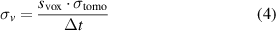
with the voxel size along one direction  given in [mm voxel−1] and the used time separation Δt given in seconds. The uncertainty regarding the velocity measurement was estimated in accordance with equation (4). A total of 1000 × 1000 × 500 voxels were used for 500 × 500 × 250 mm3 in physical space resulting in a voxel size of
  mm voxel−1. Taking the realized time separation of Δt = 0.150 s into account leads to the upper limit in terms of the uncertainty of the velocity measurement of
  mm s−1. As shown in figure 7, the instantaneous velocity distribution reached values up to
  mm s−1 resulting in a dynamic range of more than 24 levels for the velocity measurement.
With a density similar to the density of water ( kg m−3), the following behavior of the TLC seeding particles was investigated by employing the Stokes number (St) [38]
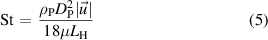
with µ being the dynamic viscosity, a characteristic velocity  and the particle diameter
  . The criterion
  determines the limit for feasible following behavior of the particles within the flow. To investigate the highest St possible within the system,
  is chosen as
  mm s−1 resulting in St = 0.007 thereby fulfilling the criterion. Thus, it is apparent that the following behavior of the TLC particles does no affect the velocity measurements.
The uncertainty of the measured temperature fields depends on the accuracy of the calibration temperature  , of the determination of the hue values in the interrogation windows
  and of the analytical calibration curves
  .
.
The temperature calibration points were determined using various temperature sensors to measure the average fluid temperature. The fluid temperature during the calibration process was determined by means of a calibrated semiconductor temperature sensor in the fluid with an accuracy of 0.01 K at 20 ∘C. This measurement was supported by 32 Pt1000 temperature sensors with class AA accuracy, i.e. every single sensor yields an accuracy of approximately 0.1 K, or combined 0.018 K. This provided a combined measurement accuracy slightly better than  K.
K.
Determining the hue values in an interrogation window implies an associated uncertainty  , which was defined by the width of the Gaussian distribution while estimating the central hue values
  . The uncertainty was estimated using the 2σ interval of this distribution, which means that 95 % of the data is described well, to derive the variation of the temperature response for all calibration curves. The largest deviation of all curves was assumed to be the upper limit for
  . The dominant uncertainty resulted from determining the central hue values Hc
for the interrogation windows:
. The dominant uncertainty resulted from determining the central hue values Hc
for the interrogation windows:  K.
K.
The subsequent determination of the analytical calibration curves was also subject to an uncertainty and amounts to  and turned out to be negligibly small:
  K.
K.
Following the Gaussian error propagation, which assumes uncorrelated uncertainties, the combined uncertainty amounted to  K. This corresponds to a high dynamic range of 21 levels for the studied temperature measurement range of 2 K. Temperature regions of specific interest can be addressed directly by using specifically tailored TLC particles with a corresponding temperature range—which, however, may result in a reduced dynamic range or an altered absolute accuracy for temperature measurements.
For the current particles per pixel densities of 0.035 and 0.025 on the b/w cameras and color camera, respectively, an ambiguity during the temperature assignment occurred only for 0.1% of the temperature values and was resolved by using only the 3D coordinate of the particle closest to the camera. Thus, there was no significant effect on the temperature measurement. Yet, for higher particles per pixel densities the ambiguities will increase and this straightforward strategy could fail.
When it comes to estimating the temperature uncertainties, it should be noted that aging effects of the TLC particles could not be taken into account. However, in order to minimize unquantifiable uncertainties related to aging of particles, the measurements were carried out directly after adding the TLC particles to the water-glycol mixture. Subsequently, the T(H)-calibration was conducted based on five data points, which were chosen as a trade-off: The aim was to acquire as many T(H)-calibration points with a small deviation from the temperature equilibrium as possible while at the same time keeping the calibration process as short as possible to avoid aging of the TLC particles. It took one day for the sample to reach the thermal equilibrium, thus generating one temperature calibration point per day. The acquired calibration data allowed for three points within the linear T(H)-regime and two within the tail. Like this, the applicable temperature range could be maximized. While the main part of the measurement data is described within the linear regime, it must be noted that the calibration points within the tail region correspond to a temperature range where the TLC particles show only minor color changes in case of temperature changes.
5. Summary and outlook
It was demonstrated that simultaneous measurements of the 3D velocity and temperature fields are feasible by combining Tomo-PIV and PIT. In this respect, TLC particles serve as both tracer particles and as thermometers. The new approach is based on a workflow, which provides the 3D position of TLC particles using the intensity maps of Tomo-PIV and determines the temperature using PIT. The velocity fields were measured in the complete sample with 62 500 cm3, whereas the temperature information was obtained in a subvolume of 20 000 cm3. Low uncertainties of  mm s−1 for the velocity and
  K for the temperature measurement were achieved corresponding to dynamic ranges of 24 and 21 levels, respectively.
Applying this new technique to turbulent RBC in a rectangular sample filled with a water-glycol mixture at  and
and  allowed for the simultaneous assessment of the velocity and temperature fields for a subset of the sample. It was shown that the non-intrusive measurement of the 3D temperature and velocity distribution of a large-scale circulation in turbulent RBC is possible. The warm upstream of fluid was captured in accordance with the determined velocity fields.
In future experiments, a new color camera with a higher sensitivity, better resolution and a larger sensor can be used to gather the temperature information from the entire sample, thus allowing for a complete acquisition of the characteristics of an LSC.
Additionally, the computational requirements can be considerably reduced by using a PTV algorithm instead of the Tomo-PIV algorithm. The main challenge for this approach is that the PTV algorithm has to be able to handle large seeding densities in order to acquire sufficient information within the life span of the TLC particles.
Data availability statement
The data that support the findings of this study are available upon reasonable request from the authors.
Acknowledgment
The authors would like to thank Annika Köhne for proof-reading this work.