

Abstract
In this work, a probabilistic calibration approach has been adopted to quantify the uncertainties of the parameters and predictions of a phenomenological shape memory alloys (SMAs) constitutive model which has been used to predict the thermally induced phase transformation of Ni–Ti SMAs. Furthermore, the impact of the adopted calibration method, which enables the determination of the uncertainty bounds of the model predictions, on the design of robust engineering applications has been discussed. To this end prior to the probabilistic model calibration, a design of experiments has been performed in order to identify the most influential parameters on the response of the system and thus reduce the dimensionality of the problem. Subsequently, uncertainty quantification (UQ) of the influential parameters has been carried out through Bayesian Markov Chain Monte Carlo (MCMC). The assessed uncertainties in the model parameters has been then propagated to the model predictions using an approximate approach based on the variance–covariance matrix of the MCMC-calibrated model parameters and then an explicit propagation of uncertainty through MCMC-based sampling. The determined 95% Bayesian confidence intervals of the model predictions, by the latter methods, have been demonstrated and compared. Additionally, good agreement between the experimentally measured and model predicted SMA hysteresis loops has been observed where the experimental data are situated within the predicted 95% Bayesian confidence intervals. Finally, the application of the MCMC-based UQ/UP approach in decision making for experimental design has also been shown by comparing the information that can be gained by performing multiple repetitive experiments under identical thermo-mechanical conditions versus experiments under different conditions.
Export citation and abstract BibTeX RIS
1. Introduction
Nickel–titanium (Ni–Ti) alloys are one of the most common shape memory alloys (SMAs), which are widely used in different engineering applications, such as biomedical devices and implants, microelectromechanical systems, sensors and actuators, seismic protection tools, and aerospace products and structures [1, 2]. Such applications are enabled by either the shape memory effect or super-elasticity, which in turn are the result of a reversible thermoelastic martensitic transformation that is triggered by applying thermal and/or mechanical loads [3, 4].
The macroscopic thermal actuation response of SMAs enables actuators with high specific weight ratio compared to the conventional alternatives [5, 6]. Thermal actuation can occur during thermal cycles under iso-baric condition where inelastic strain is recovered through the forward and reverse martensitic phase transformation induced during cooling and heating [7]. However, the forward and reverse transformations take place at different temperatures due to energy dissipation during this cyclic thermal process [8], which results in a hysteresis loop in strain-temperature space.
Under the framework of integrated computational materials engineering, completing the loop along the process–structure–property–performance chain through multiscale modeling is a necessary (albeit not sufficient) condition for the efficient and robust design of materials for specific applications. In the case of Ni–Ti SMAs, different thermodynamics and kinetics modeling are usually applied to connect process and structure, such as calculation of phase diagram (CALPHAD) [9, 10], precipitation of secondary phases [11, 12], and phase field models [13–15]. In regard to the structure-property linkages, a number of constitutive models have been proposed over the recent decades to predict the thermo-mechanical response of Ni–Ti SMAs. These models can be categorized into phenomenological [16–25] or micromechanical-based models [7, 26–29] which have been reviewed thoroughly by Patoor et al [8] and Lagoudas et al [30]. Generally, micro-mechanical models are high-fidelity and expensive models that use microstructural information to predict the macroscopic behavior of SMAs while phenomenological models are cheap and fast since the free energy associated with a non-microscopic homogenized material volume is taken into account for the prediction of the macroscopic responses [21].
Despite a substantial number of constitutive models for the response of SMAs, there are a very few studies associated with analysis, calibration, and uncertainty quantification (UQ) of the model parameters and subsequent uncertainty propagation (UP) from these parameters to the model responses. In this regard, the sensitivity of the design outputs to the uncertainty of the design input variables has been evaluated for SMA morphing structures by Oehler et al [31] through an iterative procedure based on a quasi-Monte Carlo simulation. Martowicz et al [32] also performed some preliminary work on the sensitivity analysis (SA) and UQ of a finite element based numerical model aided by meta-modeling which predicts the phase transformation response of a SMA bumper due to external thermal and mechanical stimuli. In this work, the influential input variables and the uncertainty of the output variables have been determined using central finite difference approach and Monte Carlo simulation, respectively. In another work, Enemerk et al [33] have applied an adaptive Markov Chain Monte Carlo (MCMC) approach to quantify the parameter uncertainties and correlations of a thermo-mechanical model which predicts the cyclic response of helical springs made of pseudo-elastic SMAs. Generally, it should be noted that lack of thorough sensitivity and uncertainty analysis in computational modeling is a general issue in different areas of materials science and engineering. For this reason, our developed UQ and UP frameworks have recently been applied for plastic flow behavior in TRIP steels [34] as well as CALPHAD modeling [35] to spread the use of these frameworks and show their importance in computational materials design.
Generally, uncertainties can result from different sources, including natural uncertainty (NU) from the random nature of the system, model parameter uncertainty (MPU) due to lack of knowledge and data about the model parameters, and Model structure uncertainty (MSU) as a result of incomplete or simplified physics in the model [36]. For example, the cyclic thermomechanical responses of an SMA material with the same chemistry and processing history can be slightly different during exact replications of an iso-baric experiment due to the inherent randomness (NU) in the system. In addition, there are different physical parameters in the phenomenological- or micromechanical-based models, such as transformation temperatures, which have some uncertainties (MPU) in their experimental measurements. It should be noted that physical models are usually incomplete and unable to capture all the physics in the system, including the existing thermo-mechanical models. For example, MSU in most of these models can be attributed to the absence of smooth phase transformations at austenite/martensite start and finish temperatures, independency of the applied stress to the maximum transformation strain at low stress levels and/or independency of the transformation hysteresis area to the applied stress in the prediction of the cyclic thermo-mechanical behavior of SMAs. Although the thermo-mechanical model in the current work (described in section 2) addresses the above-mentioned modeling deficiencies, the model assumptions can still result in some MSU. The consideration of the quadratic dependency of Gibbs free energy of phases to the applied stress and linear relationship between the applied stress and transformation temperatures and between the rates of martensitic volume fraction and the transformation strain are some of the main assumptions in this model. The importance of UQ and UP, which tend to be ignored in deterministic approaches towards model parameterization, is noticeably highlighted in the case of robust design where it is sought that the system response be relatively independent of the uncertainties of its variables/parameters under the operating conditions. These inverse and forward uncertainty analyses are discussed in more detail as follows.
The estimation of model parameters in order the model outputs to predict the available (experimental) data, is an inverse problem, which can be solved through deterministic or probabilistic approaches [37]. Deterministic calibration such as the least squares approach yields a single best estimate based on the minimization of the squared difference between the model results and data, while probabilistic calibration provides probability distributions and uncertainty bounds for the model parameters. It is worth noting that in some cases different combinations of the model parameters usually lead to similar model outputs, but, by definition, deterministic calibration only arrives at one best estimate. Probabilistic calibration, on the other hand, provides an ensemble of possible combinations of model parameter values in the form of probability distributions [38].
In different engineering fields, deterministic approaches have commonly been used to calibrate the model parameters leading to deterministic model predictions. However, it is widely recognized that probabilistic calibration approaches can result in more informative predictions because they enable the quantification of the uncertainties of the model parameters which can be subsequently propagated to the model results, thus offering model predictions with defined uncertainty/confidence bounds [39]. To this end, provided the design requirements of a particular application, the latter models can be used to perform robust design by designing the components associated with the application such that they meet the design requirements despite the variability on the model predictions due to the uncertainties of the model parameters. On the other hand, the deterministic models cannot lead to robust designs due to the lack of information regarding the uncertainties of their parameters and predictions.
Among probabilistic approaches, Bayesian-based MCMC algorithms have become the most commonly used tools due to the fast development in computing capabilities [40]. These sampling techniques are more robust and simpler compared to the traditional analytic and numerical approaches to solve high-dimensional intractable integrals in the probabilistic calibration process [41, 42]. In addition, MCMC methods can be used to sample from complex multivariate distributions that are usually very hard to sample using other sampling techniques such as inversion or rejection sampling [42].
MCMC sampling, however, is an expensive method, particularly in high-dimensional cases where the parameter convergence in the calibration process can be very time-consuming. A reduction in the dimensionality of the parameter space through SA, however, can significantly improve the MCMC calibration efficiency. SA is often applied to determine the impact of the parameters' variability/uncertainty on the total variability/uncertainty of the model results [43] in order to find the insensitive model parameters that can be eliminated from the calibration process. In this regard, design of experiments (DOE) is the most common approach, which requires a description of experiments (such as complete factorial design (CFD) offered by Fisher [44] or fractional factorial design to consider possible combinations of pre-defined parameters' levels) besides a subsequent analysis of the experiments (such as analysis of variance, ANOVA).
In a robust design, the final results of the model and their corresponding uncertainties are the main interest. Therefore, a UP technique should be applied by considering the trade-off between cost and information loss to propagate uncertainties from the model parameters to the model outputs [45]. This forward problem can approximately be solved through different methods with different cost and precision, e.g. forward model analysis of the parameters' optimal combinations, statistical second moment methods, polynomial chaos expansion, etc.
In the present work, the parameter SA and MCMC calibration have been performed for the phenomenological constitutive model proposed by Lagoudas et al [21]. This model has been selected due to the consideration of three important features in SMAs which are usually ignored in this type of modeling: (1) the smooth transitions in thermo-mechanical responses of SMAs during forward and reverse phase transformations that take place in a range of temperatures and/or mechanical loadings, (2) the dependency of maximum transformation strain after full transformation on the magnitude of the applied stress, and (3) the definition of a critical driving force in terms of the magnitude of the applied stress and the transformation direction [21]. In section 2, this thermo-mechanical model is described thoroughly. In section 3, parameter SA using the combination of CFD and ANOVA are explained in details and subsequently utilized to perform the sensitivity assessment of the model parameters. In section 4, the applied MCMC sampling algorithm is described and used to probabilistically calibrate the influential model parameters, and then the parameter uncertainties are propagated to the model outcomes using different UP approaches. In section 5, the information gain of two experimental designs are compared together using the relative entropies obtained after the sequential MCMC training of the model parameters with two different synthetic data-sets. This is followed by the summary and conclusion in section 6.
2. Description of the constitutive thermo-mechanical model
In this section, the phenomenological SMA constitutive model proposed by Lagoudas et al [21] is described in detail. The capability to predict the thermo-mechanical responses under general temperature-loading paths for wide ranges of SMAs with different processing histories makes this model powerful and usable for different applications. In the previous models [22, 46, 47], this capability could be achieved by high modeling cost due to increased complexity or parameter numbers.
In this model, a total Gibbs free energy is defined for the SMA material during the phase transformation in terms of the thermos-elastic contributions of austenite (GA), martensite (GM) and their interaction (Gmix) as follows,

where the external state variables σ and T are the applied stress tensor and the absolute temperature, and the internal state variables  t, ξ, and gt account for the inelastic strain produced during forward/reverse martensitic transformation, the total volume fraction of martensite which accounts for all martensitic variants, and the transformation hardening energy, respectively. Moreover, GA, GM, and Gmix according to Lagoudas et al [21] can be written as follows,

The constant parameters ρ and α are the alloy density and the thermal extension tensor, and the phase-dependent parameters S, c, s0, and u0 corresponds to the compliance tensor, specific heat, specific entropy, and specific internal energy, respectively. It should be noted that the superscripts A and M denote quantities corresponding to the austenitic and martensitic phases while the notation (. : .) shows the inner product of two second-order tensors.
The present phenomenological SMA model captures the effective response of the SMA material without considering the detailed microscale behavior of the martensitic variants. Hence any change in the microstructural state of the material is depicted macroscopically by the change of the scalar quantity ξ. To this end the evolution equations of internal state variables t and gt are defined in terms of rate of ξ. The evolution equation of t is given as [21],
where  represents the transformation direction tensor, which is expressed for both directions as

 is the effective stress where
  is the deviatoric stress, and Hcur is the maximum transformation strain after full martensitic transformation as a function of the effective stress,

where Hsat is a saturated value for the maximum transformation strain at sufficiently high value of the effective stress, and the parameter k determines the exponential rate of Hcur variation from 0 to Hsat [7, 21].
In the same manner, the evolution equation of gt is given as
where ft is a direction-dependent hardening function, which has been introduced in this model in order to capture the smooth transitions from the elastic to transformation regimes and vice versa. The expression of ft for the forward and reverse transformation is given as follows,
where ni can take values in the range of (0, 1]. The value of ni closer to zero corresponds to more smooth transition at the beginning or the end of the forward phase transformation (in the case of i = 1 or 2, i.e. n1 or n2) or their counterparts for the reverse phase transformation (in the case of i = 3 or 4, i.e. n3 or n4).
Provided with equations (1)–(8), the first and second law of thermodynamics can be utilized to derive the remaining model equations. Hence, at a local point in the material, the conservation of energy or first law of thermodynamics can be expressed as

where  , and r denote the internal energy rate, the heat flux vector, and the internal heat generation rate, respectively. In the same manner, the second law of thermodynamics at this local point can also be written as the Clausius–Planck inequality [48],

By multiplying the two sides of the inequality (10) by T and substituting div(q) by its equivalent obtained from equation (9), the following inequality can be obtained,

It should be noted that Gibbs free energy can be defined in terms of internal energy using the Legendre transformation, as follows,

Hence by differentiating equation (12) in respect to time and substitute the obtained expression of  in equation (11) the following thermodynamic constraint is derived,

Using the chain rule, the second law of thermodynamics can turn into

In inequality (14),  , and
, and  are three generalized thermodynamic forces. Following the Coleman and Noll approach [49] which states that the inequality (14) must hold true for every thermodynamic path, including the paths where all the variables are fixed in time except one, which is evolving, the total infinitesimal strain and entropy can be calculated and expressed, respectively, as follows,


From the same process, the following inequality can be obtained,

where the generalized thermodynamic force p can be obtained by taking the derivative of total G in equation (1) with respect to ξ,
As observed in this equation, p is proportional to  , that is the difference between the Gibbs free energy of pure martensite and pure austenite phase. Substituting equations (4) and (7) into (17) results in

where πt is the total thermodynamic force which must be positive during the forward transformation (when  ) and negative during the reverse transformation to hold the second law of thermodynamics (when
  ). In this model, this thermodynamic driving force must reach a stress-dependent critical thermodynamic driving force (Yt) in order to start and continue the phase transformation. Different values of Yt for forward and reverse phase transformation lead to a hyper-surface for each transformation direction, as follows,
where
In equation (21), Y0t is a constant, and the model parameter D indicates the dependency of the critical value for driving force on the applied stress.
In the case where the model is used to capture the response of an SMA subjected to one thermal cycle under iso-baric conditions (σ = cons), equation (15) is utilized. Hence, for the considered iso-baric conditions for any specific T, the value of the developed total strain is obtained by calculating the value of t and ξ during the phase transformations. That is achieved by solving the ordinary differential equation (4) while considering that during the phase transformations, the thermo-mechanical state of the material should stay on the surface defined by (20). To this end for a full thermal cycle where the temperature ranges from Af to Mf and vice versa, the hysteresis loop of the material can be obtained.
It is worth noting that the model parameters  , and D can be considered for calibration. Among these parameters, ΔS are obtained by EA/M and νA/M; and the materials properties
  , and D are associated with
  , and Hsat through relations reported in [21]. Note that EA/M and νA/M denote the Young's modulus and Poisson's ratios of austenite/martensite phases respectively while CA/M denote the slopes of the lines that define the austenitic/martensitic transformation temperatures (As/f/Ms/f) in the stress–temperature phase diagram [7, 21]. Therefore, assuming Δα and Δc as fixed parameters, EA/M, Ms, Mf, As, Af, CA/M, Hsat, k, n1, n2, n3, and n4 are the candidates for the model calibration against the existing experimental data.
3. SA of the model parameters
Before model calibration, SA is usually required to reduce the dimensionality of the parameter space with minimum possible loss of information about the model outcome in order to save calibration time and cost as a result of faster convergence of the model parameters. In this work, we carried a DOE based on a CFD coupled to ANOVA in order to identify the parameters most highly correlated to the output of the model.
3.1. Complete factorial design
CFD is an experimental design method that considers all possible combinations of R predefined levels for N factors (parameters in the case of parameter SA) in a given system/model, which is equivalent to RN level-factor combinations. In the case of parameter experimental design, model response should be obtained for each level-parameter combination for the sake of sensitivity assessment.
Based on the expert's intuition, 14 parameters have been considered as candidates for model calibration. Two plausible values have been selected for each parameter as lower and upper levels in the context of two-level CFD. These levels are considered as the applied initial values ±10% of the range of the parameters in order to hold the following temperature constraints for their design combinations,

Therefore, 214 = 16384 level-parameter combinations can be constructed during CFD whose responses are determined through the difference between the hysteresis loop obtained from running the model with each parameter combination and a reference hysteresis loop obtained using the average value of lower and upper levels of the parameters. It is worth noting that any reference curve can be applied in so far as it is consistent for all the responses. Tschopp et al [50] have evaluated various approaches to determine the similarity/difference of two images by comparing two vectors which represent the image features. In our case, these vectors were constructed based on the coordinate of spatial points on the resulting hysteresis loops,

Now, the CFD results can be applied for SA of the given model parameters through ANOVA.
3.2. Analysis of variance
A 14-way ANOVA has been performed in this work using 'anovan' function in Matlab Machine Learning toolbox, where N is the number of independent Model Parameters—see the appendix.
ANOVA is a statistical hypothesis testing technique based on the deviation associated with each individual level of each factor or each level combination of each interaction between factors in the system from the overall mean of responses. The resulting response for each one of 214 factorial design combinations has been used in the 14-way ANOVA to evaluate the sensitivity of 14 model parameters introduced in section 2. The ANOVA results associated with each parameter are shown in table 1. In this table, the model parameters have been ranked based on their corresponding p-values in descending order, which indicate the parameters from the highest to the lowest sensitivity. According to the significance level 0.05, the first eight parameters have been selected for further uncertainty analysis in order to reduce the computational cost for the model calibration that will be discussed in section 4.1. It is worth noting that the values considered as upper and lower levels in the ANOVA process, should be chosen carefully before the initiation of the process, since they may affect the estimated sensitivity of the model to some of these parameters. For example, it seems that the selected lower values of the levels for the parameter CM result in a much lower influence of this parameter on the model results compared to the parameter CA. Furthermore, another aspect which may affect the results of the SA are the loading conditions under which the considered model is evaluated during this process. In the current example, the model sensitivity has been determined using iso-baric loading paths. In these conditions, the sensitivity of the model on the value of the EM and EA is minimized since the response of the model under the selected conditions is dictated mainly due the thermally induced phase transformation. In the current work, we selected the iso-baric loading path due to the focus on the UQ of the thermal phase transformation related model parameters.
Table 1. ANOVA table results showing the model parameters ranked based on their p-values in descending order.
| Source | Sum sq. | d.f. | Mean sq. | F | Prob > F |
|---|---|---|---|---|---|
| Hsat | 0.659 41 | 1 | 0.659 41 | 800.62 | 5.3041e-172 |
| Af (K) | 0.332 78 | 1 | 0.332 78 | 404.05 | 8.5195e-89 |
| Ms (K) | 0.089 07 | 1 | 0.089 07 | 108.14 | 3.0049e-25 |
| Mf (K) | 0.044 02 | 1 | 0.044 02 | 53.45 | 2.7735e-13 |

|
0.034 88 | 1 | 0.034 88 | 42.35 | 7.8628e-11 |

|
0.024 62 | 1 | 0.024 62 | 29.90 | 4.6223e-08 |

|
0.010 29 | 1 | 0.010 29 | 12.50 | 4.0821e-04 |
| As (K) | 0.003 23 | 1 | 0.003 23 | 3.93 | 0.0476 |

|
0.000 18 | 1 | 0.000 18 | 0.21 | 0.6443 |

|
0.000 08 | 1 | 0.000 08 | 0.09 | 0.7612 |
| n1 | 0 | 1 | 0 | 0 | 1 |
| n2 | 0 | 1 | 0 | 0 | 1 |
| n3 | 0 | 1 | 0 | 0 | 1 |
| n4 | 0 | 1 | 0 | 0 | 1 |
| Error | 13.481 9 | 16369 | 0.000 82 | ||
| Total | 14.6805 | 16383 |
4. Bayesian UQ and UP of the model parameters
4.1. Parameter estimation and UQ using MCMC-Metropolis Hastings (M–H) Algorithm
In order to sample the parameter space, one can use MCMC sampling approaches [42]. Among these approaches, (M–H) sampling is one of the most common applied tools to probabilistically solve the inverse problem associated to the probabilistic parameter calibration given experimental data. In the case of model calibration, this technique updates the existing prior knowledge about the parameters to their posterior information based on the available data for the model responses.
In the present work, MCMC toolbox in Matlab has been used to probabilistically calibrate the eight sensitive model parameters identified in section 3.2. First, the prior parameter information, including the initial values (θ0), valid ranges, and probability density functions (PDFs) for the parameters are considered. Then, a new parameter vector/candidate θcand is randomly sampled from a proposal posterior PDF (q) which is defined as a multivariate Gaussian distribution in the toolbox with a mean value at θ0 and an arbitrary variance–covariance matrix. The candidate is accepted/rejected using a probabilistic criterion defined based on the M–H ratio that is expressed as follows,

In this equation, the first ratio is called Metropolis ratio which is the ratio of the posterior probability of θcand to θ0 given data (D). In the context of the Bayes' theorem, the posterior probabilities are proportional to the prior probability times the likelihood—probability of the data given model results evaluated with the candidate model parameters—for each case. We considered the likelihood to be a Gaussian distribution centered at the data whose error is considered as the distribution variance. In the case of multiple data sets, it should be noted that the product of the likelihoods obtained from each data set can yield the total likelihood if data sets are assumed to be conditionally independent.
The Metropolis ratio can be applied for the acceptance/rejection of the candidate when the proposal distribution is symmetric; however, this is not usually the case since the probability of moving from θ0 to θcand is not necessarily equal to the probability of the reverse move. For this reason, Hastings introduced the second ratio in equation (24) to involve the above-mentioned non-symmetric property of the proposal distribution [42, 51]. Now, min(MH × 100, 100) is considered as the acceptance probability of the candidate [51]. According to this criterion, If the candidate is accepted, then θ1 = θcand; otherwise, θ1 = θ0. The sampling of the new candidate and its acceptance/rejection process are sequentially repeated n times by finding the M–H ratio using the new sampled candidate and the previous accepted parameter during each iteration. At the end of the procedure, n samples of the parameter vector ( ) are generated to represent a multivariate posterior distribution for the model parameters.
Before the convergence of the parameter samples, samples generated during the 'burn-in period'—in which the different samples are causally correlated—must be removed before further analysis of the parameters. After the removal of the burn-in period, the mean values and the square root of diagonal elements in variance–covariance matrix of the remaining samples in the convergence region can be introduced as the plausible optimal values and uncertainties of the model parameters.
In our calibration work, initial values and their ranges have been determined based on the expert's beliefs, and an uniform (non-informative) probability distribution has been selected for each model parameter due to the absence of knowledge about the parameters' PDF. In addition, three experimental datasets for transformation strain-temperature hysteresis loop under different iso-baric conditions have simultaneously been utilized together to calibrate the model. It is worth noting that the experimental iso-baric response of SMAs has been obtained using SMA dog-bone specimens. The specimens were uniaxially loaded at the stress levels under iso-thermal conditions above the Af temperature. Subsequently, they have been thermally cycled between a temperature below the Mf and a temperature above the Af at a constant stress [52]. The calibration has been performed through the calculation of the difference between various iso-baric hysteresis curves obtained from each parameter sample and the corresponding experimental data using equation (23). For the sake of the parameter calibration, these differences (discrepancies) resulting from three given iso-baric conditions ([M(θ)]1×3) are simultaneously compared with a zero vector (D = [0 0 0]) in the likelihood function.
In this work, the likelihood variance σ2 (the squared error of the distances between model and experimental hysteresis curves from zero) is set as an unknown hyper-parameter in the calibration process and updated in parallel with the other model parameters during MCMC sampling. The only difference is that an inverse-gamma distribution is defined as the non-informative prior PDF for this hyper-parameter, which yields the same form of distribution for the posterior PDF after applying the Bayes' theorem since the inverse-gamma distribution is the corresponding conjugate prior density for exponential likelihood functions. Therefore, σ2 is sampled from an inverse gamma posterior distribution during MCMC process [53]. In addition, it should be noted that an adaptive proposal distribution has been employed in this calibration work. In this scheme, an arbitrary positive covariance (V0) is selected in the beginning of MCMC sampling, and then it is adapted in each next iteration using the covariance obtained from the ensemble of previous samples in the MCMC chain [54, 55].
In this work, a constrained MCMC approach has also been developed in order to consider the constraints for the transformation temperatures mentioned in equation (22). For this purpose, the likelihood is penalized by assigning an infinitely high value for the distance between model and experimental hysteresis curves in the cases that the constraints for the parameters are not satisfied. In these cases, the induced penalty results in a likelihood close to zero, which in turn results in an infinitesimally small acceptance probability for new model parameter candidates that violate constraints.
In the calibration of the sensitive model parameters, high number of samples (i.e. 200 000) are generated to ensure the convergence of the parameters and the uniqueness of the optimal response in the parameter space. The multi-variate posterior distribution after MCMC sampling can be assessed through joint and marginal frequency distributions. In figure 1, some of the parameter joint distributions have been shown in 2D color graphs as examples, where the colors represent different density of samples in the parameter space, increasing from blue to red spectra. These types of graphs can also demonstrate the correlation between each pair of parameters qualitatively. For instance, negative/positive linear correlations can be inferred from the negative/positive slopes of the elliptical shapes in the graphs. The linearity of the sample distribution in the parameter space can be determined quantitatively through Pearson correlation coefficient ( ) that is expressed as

where σX and σY are the standard deviations for parameters X and Y, respectively, which equal the square root of the corresponding diagonal elements in 8 × 8 variance–covariance matrix. cov(X, Y) is also the covariance of X and Y obtained from the corresponding non-diagonal element in the variance–covariance matrix. Generally, a value of ρ closer to either −1 or 1 implies a higher linear correlation between X and Y, whereas a value closer to zero suggests their lower linear correlation. The negative or positive sign refers to the negative or positive linear correlation. The linear coefficients for all pairs of parameters in the thermo-mechanical model have been listed in table 2. As can be observed in this table, most of the pair parameters are linearly uncorrelated although 6 out of 28 parameter pairs show some weak or moderate correlations with  greater than 0.2. In addition, the parameters CA and Af (figure 1(d)) and the parameters EM and CA (figure 1(f)) show the highest and the lowfest linear correlation, respectively, regardless of the correlation signs.

Figure 1. Joint frequency distributions for some of the pair model parameters in the form of 2D color graphs with normalized color bars.
Download figure:
Standard image High-resolution imageTable 2. Linear correlation coefficient for each pair of model parameters.
| As (K) | Af (K) | Ms (K) | Mf (K) |

|

|
Hsat |

|
|
|---|---|---|---|---|---|---|---|---|
| As (K) | 1 | −0.0721 | 0.2948 | −0.1080 | 0.3813 | −0.0167 | −0.1330 | −0.0378 |
| Af (K) | −0.0721 | 1 | −0.0150 | −0.0822 | 0.5836 | −0.0553 | 0.0249 | −0.0672 |
| Ms (K) | 0.2948 | −0.0150 | 1 | −0.4628 | 0.1156 | −0.0547 | −0.0465 | −0.0415 |
| Mf (K) | −0.1080 | −0.0822 | −0.4628 | 1 | −0.1280 | −0.0289 | −0.1355 | 0.0160 |

|
0.3813 | 0.5836 | 0.1156 | −0.1280 | 1 | −0.0015 | 0.0476 | −0.0405 |

|
−0.0167 | −0.0553 | −0.0547 | −0.0289 | −0.0015 | 1 | 0.2771 | 0.0091 |
| Hsat | −0.1330 | 0.0249 | −0.0465 | −0.1355 | 0.0476 | 0.2771 | 1 | −0.2103 |

|
−0.0378 | −0.0672 | −0.0415 | 0.0160 | −0.0405 | 0.0091 | −0.2103 | 1 |
As mentioned above, the burn-in period at the beginning of MCMC sampling must be removed before the calibration and UQ of the model parameters, which can be found using the cumulative mean distributions for the parameters, as shown in figure 2. In these figures, there are some noisy trends at the beginning of MCMC sampling for the cumulative mean values of all the parameters, but they reach almost plateaus after about 63 000 generations that show the convergence values (mean values) for the parameters. Therefore, the first 63 000 samples are extracted from the total MCMC sample collection before further analysis. The mean and the square root of the diagonal elements in the variance–covariance matrix of the remaining samples in the convergence region can be introduced as the plausible optimal values and the uncertainty of the model parameters, which are listed in table 3.

Figure 2. Cumulative mean distribution plot for each model parameter after MCMC sampling.
Download figure:
Standard image High-resolution imageTable 3. Plausible optimal values and uncertainties (standard deviations) of the model parameters after MCMC calibration besides their initial values.
| As (K) | Af (K) | Ms (K) | Mf (K) |

|

|
Hsat |

|
|
|---|---|---|---|---|---|---|---|---|
| Initial values | 307.0 | 318.0 | 300.0 | 270.0 | 9.0 | 40.0 | 0.034 | 0.02 |
| After MCMC calibration | 296.6 ± 8.5 | 322.6 ± 11.3 | 280.4 ± 6.6 | 259.9 ± 8.5 | 11.8 ± 4.1 | 35.6 ± 8.6 | 0.051 7 ± 0.0044 | 0.0595 ± 0.0237 |
After removal of the burn-in period, the marginal posterior frequency distribution of the parameters can be plotted using the remaining MCMC samples as observed in figure 3. These plots suggest truncated skewed Gaussian distributions for the marginal posterior frequency distributions; although they are flatter in the case of the parameters EM, k and CA, and more close to a Gaussian distribution for the parameter Hsat.
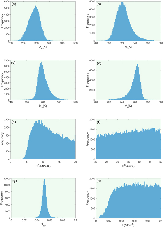
Figure 3. Marginal posterior frequency distribution plot for each model parameter after the removal of the burn-in period from MCMC samples.
Download figure:
Standard image High-resolution image4.2. UP from the model parameters to the model outcomes
As mentioned earlier, only the final results of the model and the corresponding uncertainties are considered important in the context of the robust design. The reason is that such information can help the designers to reduce the influence of the system performance by the existing uncertainties in the outcomes, regardless of how many variables and models have been involved. Therefore, an appropriate UP technique is essential to propagate uncertainties from the model parameters/input variables to the outputs with a relatively high efficiency and a minimum or at least quantifiable loss of information [45]. Among different UP methods, first/second order second moment (FOSM) approaches are probably the most common approximation procedures in engineering [56]. In this work, FOSM approach has been used to perform nonlinear propagation of the variance–covariance matrix of the model parameters.
Let θ and  vectors denote the optimal MCMC samples for the parameters (after removal of the burn-in period) and their mean values, respectively, and
  denote the model objective (output) function. If the objective function is estimated by a first order Taylor expansion at
  ,
,

The expected values associated with first and second moment of the above first order Taylor expansion approximates the mean value ( ) and variance (
 ) of the objective function M [56] as follows,


where  and σij are the variance of the parameter θi and the covariance between the parameters θi and θj, respectively. The approximations in equations (27) and (28) have been derived thoroughly by Kriegesmann [57]. It is worth noting that equation (28) can also be expressed in terms of the variance–covariance matrix of the model parameters (V) [58] as follows,

where g is a column vector which consists of all partial derivative elements, i.e.  .
.
The uncertainties of parameters reported in table 3 have been propagated to the uncertainty of the transformation strain along the hysteresis curves by applying the variance–covariance matrix obtained from the optimal MCMC samples (without burn-in period) in the above-mentioned FOSM approach. The results have been shown in figure 4 for different iso-baric conditions. In these figures, the blue/red solid and dashed lines correspond to the model results during cooling/heating process (forward/reverse martensitic transformation) and their experimental counterparts, respectively. In addition, the blue/red shaded regions indicate 95% Bayesian confidence interval (95% BCI) for model results during cooling/heating. It should be noted that the interval is equivalent to  , where εt(T) and
  can be calculated through equations (27) and (28), respectively.
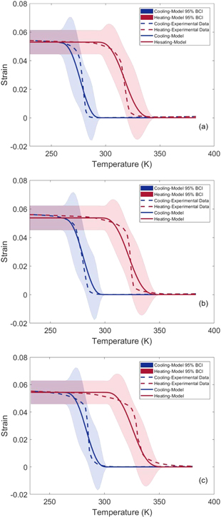
Figure 4. 95% BCIs for the model hysteresis curves obtained from the FOSM approach for different iso-baric conditions, (a) 100, (b) 150, and (c) 200 MPa, besides their corresponding experimental counterparts.
Download figure:
Standard image High-resolution imageThe average Euclidean distances between the mean strain values of the hysteresis curves obtained from the model (solid lines in figure 4) and their corresponding experimental values (dashed lines in figure 4) have been calculated as 0.0083, 0.0059 and 0.0032 for the iso-baric conditions 100, 150 and 200 MPa, respectively. As can be observed, these results show small discrepancies (good agreements) between the model and experimental hysteresis loops, or at least the experimental data are located inside the 95% BCIs based on figure 4. Although it seems that the given thermo-mechanical model underestimates the slope of the curves during forward and reverse transformation and their convergence temperatures (where cooling and heating curves meet each other), there are no discrepancies between model results and experimental data for the maximum transformation strain (Hcur) in each iso-baric condition. The difference in the curve slopes can be attributed to the slight effects of other parameters that are not considered in the calibration, the missing physics in the model, and the uncertainties in the experimental data all together.
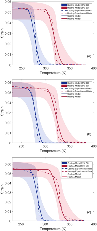
Another important feature in theses graphs are the unrealistic humps around the transformation temperatures, which can be related to the deficiency of the partial derivatives in the applied UP approach (equation (28)) at where the changes are sudden. For this reason, a direct UP has been performed using the model forward analysis of optimal MCMC samples to find more rational regions for 95% BCIs. After running the model for all the optimal samples, 2.5% of the resulting hysteresis curves have been eliminated from each one of the top and down margins to obtain the mentioned intervals. As shown in figure 5, this approach yields smoother and more precise boundaries for 95% BCIs with no humps. Assuming the 95% BCIs obtained from the direct UP as the ground truth, the average relative error of the FOSM approach has been calculated around 21%; which is based on an average of the relative differences between the corresponding upper and lower bounds of BCIs obtained in figures 4 and 5 at different temperatures and iso-baric conditions. However, these UP approaches are different in cost. The cost of the direct UP approach depends on the applied number of parameter samples which can slightly influence the accuracy of uncertainty bands obtained. Despite the wide range of cost for the direct UP approach, it can be stated this approach costs at least 30 times more than the FOSM approach in most applications. Therefore, there is a trade-off between cost and accuracy for the application of these UP approaches. The expensive direct UP approach is required in the case that the accuracy of the quantified uncertainty is highly important; otherwise, the FOSM method can be applied to reduce the UP cost.
Figure 5. 95% BCIs for the model hysteresis curves obtained from the direct UP approach for different iso-baric conditions, (a) 100, (b) 150, and (c) 200 MPa, besides their corresponding experimental counterparts.
Download figure:
Standard image High-resolution image
5. MCMC application in decision making for experimental design
In this section, the goal is to respond the experimentalists' question about which experimental design can gain more knowledge about the system: performing experiments at the same conditions or at different conditions in design input space. For this purpose, it is assumed that the probabilistically calibrated model in section 4.1 can yield the ground truth and its NU bounds at any design condition (i.e. any iso-baric condition). According to this assumption, two different synthetic experimental sets are designed through sampling the hysteresis curves from the model uncertainty bounds obtained at any iso-baric condition of interest. The first set contains three random samples (replicas) from the same experimental condition (i.e. σ = 150 MPa), while the second set considers three random samples from three different conditions (i.e. σ = 175, 250, and 300 MPa). After the generation of synthetic data sets, the calibrated results obtained in table 3 for the influential parameters are considered as the parameter priors which are separately updated against each set of synthetic data using the MCMC technique in a sequential way of data training. In this way of training, the parameter posterior distribution obtained after each training is considered as the prior distribution for the next training. The relative entropy (Kullback Leibler (K–L) divergence) is calculated to find how diverged the probability distributions are relatively, i.e. what is the distance between the prior and final posterior probability distributions of the parameters after the three sequential MCMC calibrations in each case. The calculated K–L divergence can be introduced as a comparison measure for the amount of information gained from each synthetic experimental set. Generally, K–L divergence for continuous probability distributions P and Q is defined as

where p(x) and q(x) are the densities of P and Q at any given random point x, respectively. In the case of multivariate Gaussian distribution, the integration in equation (30) can be obtained as follows,

The equivalent normal distributions obtained for parameter prior and posterior distributions are compared for each set of experimental design using equation (31). The K–L divergence values for synthetic experimental sets 1 and 2 are calculated around 3.8 and 4.4, respectively. The higher value of the K–L divergence for synthetic experimental set 2 indicates a greater difference between prior and final posterior distributions in this case, which implies that the consideration of different conditions in experimental design can gain more information about the system rather than experimental replicas in the same condition.
It is also important for experimentalists to know how much information they gain by adding each experiment. In our work, the K–L divergences obtained after each training sequence are 1.65, 0.64 and 0.60 for synthetic experimental set 1 and 3.65, 0.80 and 0.67 for synthetic experimental set 2. It is worth noting that the addition of these K–L divergences should not necessarily equal the overall K–L divergence already obtained for each set since the random generated data can not only diverges, but also converges the parameter mean values to the mean values of the parameter prior probability used in the beginning of the trainings. As can be observed in both synthetic experimental designs, the K–L divergence reduces as the training continues with more synthetic data. This trend can be attributed to a dramatic decrease in the rate of the parameter uncertainty reduction from the prior to the posterior distributions during the sequential MCMC training. This decreasing rate has the main contribution in the reduction of the prior distribution divergence from the posterior distribution as the trainings proceed. Moreover, the difference in the mean values of the prior and posterior distribution also influences the K–L divergence after each training, as shown in equation (31). Although this difference is directly affected by how far the randomly generated data are from each other in the sequence, it generally tends to reduce by adding more synthetic data. The reason being the prior distributions become more peaked and thus more dominant than likelihood during the MCMC sampling which result in less changes in the parameter mean values after each training.
6. Summary and conclusion
In this work, the calibration and UQ of the sensitive parameters in a thermo-mechanical model have been performed against three different iso-baric experimental data simultaneously using a constrained MCMC-MH algorithm in the context of Bayesian statistics. Compared to the few prior preliminary works for sensitivity and uncertainty assessment of SMAs thermo-mechanical models through central finite difference, Monte Carlo and MCMC approaches, this work proposes a global variance-based SA known as ANOVA as well as a thorough MCMC analysis of the uncertainty for model parameters and its propagation to model responses. It should be noted that the applied model is able to predict the thermo-mechanical responses of SMAs with various chemistries and processing histories under general temperature-loading paths. Besides the generality of this model in the prediction of SMA thermo-mechanical responses, it is less complex with the least possible number of parameters compared to the previous similar models, which makes the model calibration process less expensive. However, it should be noted that just the iso-baric conditions with cyclic varying temperatures are considered in this work to calibrate the model that makes its accurate predictions limited to the mentioned conditions. In order to generalize the application and predictability of this model, the parameter calibrations should be performed with much more experimental data obtained from different thermo-mechanical conditions, such as the iso-thermal conditions with cyclic varying stresses or the conditions where applied stresses and temperatures are both changing. In this work, the iso-baric conditions are used as examples to propose a UQ framework that can be applied to provide probability distributions in the form of uncertainty bands for the thermo-mechanical responses of the applied Ni–Ti SMA using the propagation of uncertainties from the probabilistically calibrated model parameters. This is very important since predicting probablistically rather than deterministically can provide confidences in the robust design of these SMAs for their specified applications.
Eight sensitive parameters have been found before the calibration using a DOE approach which includes CFD and N-way ANOVA. After MCMC sampling of these eight parameters, their convergence have been checked by the joint frequency distributions and the cumulative mean plots, which have also been utilized to identify the qualitative correlation of each pair parameters and the burn-in period, respectively. In addition, the linear correlation between each two parameters has been calculated through Pearson coefficient. These coefficients suggest that most pair parameters are linearly uncorrelated, although a few of them show weak or moderate linear correlations.
After removal of the samples belonging to the burn-in period, skewed Gaussian distributions have been obtained for the marginal posterior frequency distributions of the model parameters, which are truncated in the range defined for each parameter. Moreover, it should be noted that the mean and square root of the diagonal elements in the variance–covariance matrix of the remaining optimal samples after the elimination of the burn-in period provide the plausible optimal values and uncertainties of the selected parameters, respectively.
At the end, the parameters' uncertainties have been propagated to the uncertainties of the transformation strain along the hysteresis curves using two various UP techniques in order to find 95% BCIs during cooling/heating process. In this regard, FOSM approach results in some unrealistic humps around the transformation temperatures. For this reason, a direct UP technique has been performed through the forward analysis of optimal MCMC samples in order to achieve more rational and precise uncertainty bands that are very important in the context of robust design. The hysteresis curves obtained from the mean values of the parameters are in good agreements with their experimental counterparts for different given iso-baric conditions, or at least it can be stated that the experimental data are situated in 95% BCIs. Although the slopes and the convergence temperatures of the forward and reverse transformation curves are not predicted precisely which can be the deficiencies of the applied model, the maximum transformation strain associated with each iso-baric condition is very close to its corresponding data.
In this work, it has been also shown that the MCMC approach can be applied for decision making in experimental design. Assuming the calibrated model can predict the ground truth and the natural uncertainties in different experimental conditions, two synthetic experimental sets have been sampled from the model response uncertainty bounds obtained at the same and different iso-baric conditions, respectively. After sequential MCMC updates of parameters' posterior distributions with each set, their information gains are compared together through the calculation of K–L divergence for each case which indicate the difference between prior and final posterior distributions of the model parameters. A higher information gain has been obtained from the synthetic experimental set 2 that are sampled from different experimental conditions (different iso-baric conditions). It has also been shown that the K–L divergence and its rate reduce as the sequential training proceeds in both synthetic experimental designs.
Generally, this work introduces a complete framework for UQ of model parameters and subsequent UP from model parameters to outputs as a guideline for material design.
Acknowledgments
The authors would like to thank the support of the National Science Foundation (NSF) through the Designing Materials to Revolutionize and Engineer our Future (DMREF): grant no. CMMI-1534534.
Appendix. Two-way ANOVA
In the case of two-way ANOVA where there are L observations and two multi-level factors A and B, system response can be defined as a Means model as follows [59],
where I and J are the number of levels associated with factors A and B, and τi, βj, and (τ β)ij denote the effects of the level i of factor A, level j of factor B, and their interaction, respectively. is the residual or the random error which is considered as an independent normally distributed function with a fixed variance,  . In this context, the following hypotheses are statistically evaluated to find the most sensitive factors and interactions in the system [59],


In each case, H0 and H1 are null and alternative hypothesis, respectively. It should be noted that a component (either a factor or an interaction) is identified sensitive when the corresponding null hypothesis is rejected after hypothesis testing. In this regard, a variance partitioning into the components of the system is required; however, this partitioning can be performed on the total sum of squares instead due to the proportionality between total variance and total sum of squares.
Let yi.., y.j., yij., and y... denote the sum of all the factorial design responses which includes the effects of the level i of the factor A, the level j of the factor B, the combination of the level i for A and the level j for B, and all the level-factor combinations, respectively. Moreover, let  , and
, and  denote the corresponding averages as follows [59],


Total sum of squares (SST) can be decomposed to the sum of squares of the system components, as follows,
where SSA, SSB, SSAB, and SSE are the sum of squares associated with A, B, A–B interaction, and the random error, respectively. It is worth noting that SSE can be obtained by the subtraction of SSA, SSB, and SSAB from SST. In equation (40), the first equality results from the addition and subtraction of the same terms on the right side, and the second equality is a consequence of the polynomial expansion of the function where the six cross products becomes zero. If these sum of squares are divided by their corresponding degrees of freedom, the mean squares (MS) are obtained. The expected values of these mean squares when the levels are random variables can provide relationships to estimate the total deviations of all the levels associated with A, B, and A–B interaction, as follows,


It should be noted that the mean square of each factor or interaction can be used in the above equations in the problems that the levels are fixed. In the case that the null hypothesis about the insensitivity of a factor or an interaction is true, the total corresponding effects of the component becomes zero; therefore, the corresponding expected value in equations (41), (42) or/and (43) equals the expected value for the mean squares of the random error, i.e. its variance (σ2). On the other hand, if there are any effects from the system components, the corresponding expected values are greater than σ2. It is clear that bigger ratio of the expected value of a component to σ2 is equivalent to more sensitivity of the component. This is also true for the ratio of the corresponding mean squares, which is called F-ratio. However, a certain criterion is required to fully reject the null hypotheses for the identification of the sensitive components in the system. For this reason, a F-distribution is created from anyone of the null hypotheses based on the numerator and denominator degrees of freedom of F-ratio to calculate the corresponding p-value. Generally, the area underneath the F-distribution confined between the F-ratio value and infinity is introduced as the p-value. Different significance levels can be set as the criteria to reject the null hypotheses, i.e. 0.01, 0.05, or 0.1. For any system component, a p-value less than the significance level rejects the corresponding null hypothesis, and demonstrates the sensitivity of the given component.
In the case that there is just one observation/response for each level-factor combinations (generally for the models and simulations where their response is deterministic such as our thermo-mechanical model), the variance of the random error (σ2) can not be determined by the expected mean squares of the random error in equation (44) since L equals 1. Under this condition, no clear differentiation can be established between the effect of the interaction and the random error in equation (43). Therefore, the interaction effect in equation (32) must be considered zero in order to be able to estimate σ2 using equation (43); otherwise, the effect of each individual factor can not be estimated through equations (41) and (42). ANOVA table for this case can be observed in table A1 [59].
Table A1. Two-way ANOVA table for the case of one observation/response per level-factor combination [59].
| Source of | Sum of | Degrees of | Mean | Expected mean | F- |
|---|---|---|---|---|---|
| variation | squares | freedoms | square | square | ratio |
| A |

|

|
MSA |

|

|
| B |

|

|
MSB |

|

|
| Residual or AB | Subtraction |

|
MSE |

|
|
| Total |
|

|