

Abstract
Silver nanowires (Ag NWs) are a promising material for building various sensors and devices at the nanoscale. However, the fast and precise placement of individual Ag NWs is still a challenge today. Atomic force microscopy (AFM) has been widely used to manipulate nanoparticles, yet this technology encounters many difficulties when being applied to the movement of Ag NWs as well as other soft one-dimensional (1D) materials, since the samples are easily distorted or even broken due to friction and adhesion on the substrate. In this paper, two novel manipulation strategies based on the parallel pushing method are presented. This method applies a group of short parallel pushing vectors (PPVs) to the Ag NW along its longitudinal direction. Identical and proportional vectors are respectively proposed to translate and rotate the Ag NWs with a straight-line configuration. The rotation strategy is also applied to straighten flexed Ag NWs. The finite element method simulation is introduced to analyse the behaviour of the Ag NWs as well as to optimize the parameter setting of the PPVs. Experiments are carried out to confirm the efficiency of the presented strategies. By comprehensive application of the new strategies, four Ag NWs are continuously assembled in a rectangular pattern. This study improves the controllability of the position and configuration of Ag NWs on a flat substrate. It also indicates the practicability of automatic nanofabrication using common AFMs.
Export citation and abstract BibTeX RIS
1. Introduction
Silver nanowires (Ag NWs) are possible building blocks for many nanodevices due to their regular geometry, unique physical properties and ease of synthesis [1–3]. For instance, they can be integrated into wearable sensors and stretchable devices due to their excellent flexibility and high conductivity [4–6]. In recent years, Ag NWs have also found applications in nanophotonics and nanoelectronics, and they have been used as waveguides, transistors, switches and logic gates [7–9]. The precise placement of individual Ag NWs is an essential premise of assembling nanodevices. However, this is still challenging today. The atomic force microscope (AFM) is considered to be the most popular tool so far for manipulating objects at the nanoscale. It has been applied to the movement and bending of various 1D materials and to the further investigation of the friction between different materials and substrates [10–13]. However, because of its low efficiency, this technology is rarely used to assemble complex patterns of nanomaterials. The AFM probe cannot be operated in imaging mode and manipulation mode simultaneously; therefore, the manipulation process is essentially invisible. In order to determine the object's position and to further plan the next movement of the probe, the image has to be updated after each manipulation step. Since it usually takes minutes to capture an image with conventional AFMs, multi-step manipulation is extremely time consuming and hence not acceptable for productive application. A few techniques, such as the AFM-electron microscopy combination system, the virtual reality nanorobot and the dual-probe AFM, may help to increase efficiency by visualizing the manipulation [14–18]. Nevertheless, these techniques have not been commonly used so far due to the requirement of more sophisticated equipment as well as some advanced operation skills.
In recent years, we have developed an automated nanomanipulation technology for general AFM systems [19]. The idea is that the manipulation results of each manipulation step are predicted by theoretical modelling instead of real-time imaging; therefore all manipulation steps are allowed to be implemented continuously without intermediate scanning. In this way, the total time consumption of the complex manipulation can be significantly reduced. This technology has been used to manipulate low-aspect-ratio multi-walled carbon nanotubes (MWCNTs), which behave like rigid rods [20]. Due to their high bending stiffness, the geometric configurations of these samples are well maintained during manipulation. By alternately pushing the two ends of the MWCNT, it can be 'swung' to a pre-assigned position on the substrate with high accuracy and efficiency. Nevertheless, the reported strategy is improper for nonrigid samples like Ag NWs, because the flexible 1D material is likely to be severely distorted or even broken after manipulation.
The present work aims to develop new manipulation strategies for Ag NWs with a common AFM. Since the straight line shape is the simplest ideal geometric configuration for building an electronic connection, this paper focuses on the discussion of transferring straight Ag NWs. The strategies include translation and rotation, which are the two basic manipulation techniques for moving a 1D material. For simplicity, the manipulation is limited to a symmetrical flat surface.
2. Modelling and strategies
2.1. Mechanical model
An NW manipulated by an AFM probe is often considered to be a beam lever under concentrated and distributed force loads [21–24], where the concentrated load represents the pushing force from the AFM probe, and the distributed load represents the friction on the substrate. Nonrigid 1D materials, like Ag NWs, are usually partly bent by a single push manipulation. Assuming that the pushing force is perpendicular to the NW and the displacement is short, then at each moment during the pushing process the bending part of the NW can be modelled as a fixed–fixed beam, as shown in figures 1(a)–(b). If the ends of the NW are not moved in this process, the bending part is symmetric about the force application point. The frictional force acting on this part is dynamic friction, which is supposed to be equivalent everywhere along the curved NW. The other parts of the NW are fixed by unevenly distributed static friction. According to the elastic mechanics, the curved segment of the NW can be described by the following deflection equations of Euler's beam:
where E and I are the elastic modulus and sectional area moment of inertia of the NW, l is the initial length of the curved segment, q is the dynamic frictional force per unit length, F is the pushing force and (x, y) are the coordinates of each point on the curved segment in the coordinate system marked in the graph. Because the shear forces at the two ends of the curved segment are always small in this situation, the pushing force F is approximately balanced by the dynamic friction, namely F ≈ ql. Thus the deflection of the NW at the force application point can be given by:

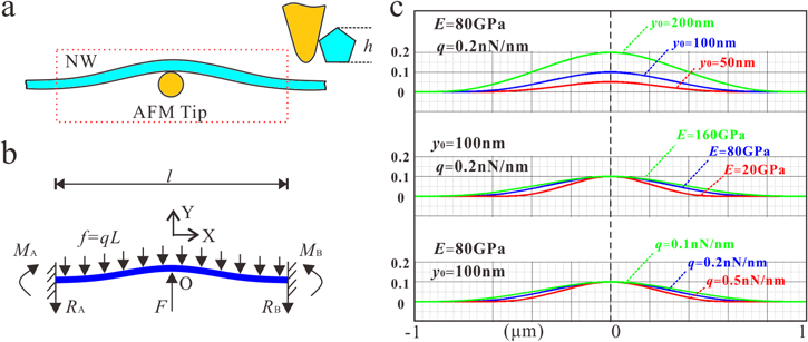
Figure 1. A mechanical model of the NW under a single push. (a) A schematic illustration of the partly bent NW; the segment in the dashed box is bent while the other parts remain at the initial position. (b) Force analysis of the curved segment. Supposing the manipulation process is quasistatic, the curved segment can be considered as a fixed–fixed beam in balance. RA, RB, MA and MB are the shear forces and the bending moment at the two ends of the curved segment, respectively. RA and RB are small compared to the dynamic friction f. (c) The variation of the NW's shape with a different pushing distance, elastic modulus and dynamic friction. The total length shown in the plot is 2 μm. The curved segment is within this region, and the area moment of inertia I = 0.0484h4, where h is the height of the NW, equivalent to 50 nm in this plot.
Download figure:
Standard image High-resolution imageIn most AFM-based manipulation, the actively controlled argument is the displacement rather than the pushing force. So the length of the curved NW is actually the function of the deflection at the force application point as well as the mechanical properties of the NW and the friction. To clear this relationship, equation (2) is converted into the following form:
By substituting equation (3) into equation (1), the whole profile of the curved NW can be determined. It is known from the above equation that a longer pushing distance will bend a larger segment of the NW. Meanwhile, the higher elastic modulus and the area moment of inertia will also result in deflection in a wider part of the NW. In contrast, the friction always hampers the movement of the NW and impedes the extension of the bending part. Figure 1(c) depicts how these parameters respectively influence the shape of the NW.
When the pushing force is retracted, the NW may remain at the new position or rebound back depending on whether the static friction is strong enough to hold the NW. Let qs be the maximum static frictional force per unit length of the NW, and φ and s be the local slope angle and the arc length of the NW at the last moment before the probe is withdrawn; then the following formula can be used as a judgement:

If the above formula is true at any point on the curved NW, its shape can be well maintained; otherwise rebounding will happen.
2.2. Translation and rotation strategies
The above analysis indicates that the nonrigid 1D material will always deflect when it is moved by only one push action. Therefore, we suppose that the Ag NW should be re-straightened after multiple push actions despite being bent during the process. A possible strategy for this is using a group of parallel pushing vectors (PPVs) to move the NW section by section. The effect of the PPVs on the shape of the NW may be understood simply looking at figure 2, where two pushing vectors of the same length and direction are applied to the NW in sequence. The vector executed first P1 bends segment A1B1, and the following vector P2 causes the deflection of segment A2B2. Supposing formula (4) is satisfied, the curved NW is well held by the substrate. If the distance between P1 and P2 is shorter than the length of the curved segment, A1B1 and A2B2 partly overlap. The deflection of each point in the overlap region mainly depends on the larger value of the two deflections respectively induced by P1 and P2. If these two vectors are close enough, the NW between them will approach the straight line connecting the ends of P1 and P2. If a number of PPVs are applied in this way, all the NW segments between adjacent vectors will be approximately on the same line.
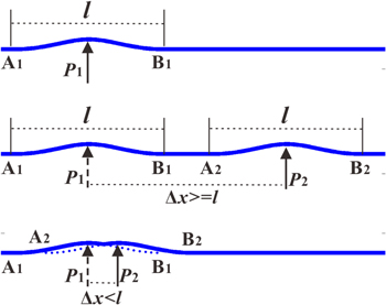
Figure 2. A schematic illustration of the effect of two PPVs. P1 and P2 are the two pushing vectors, l is the length of the segment bent by each vector, Δx is the distance between the two vectors.
Download figure:
Standard image High-resolution imageBased on the above discussion, a translation strategy is proposed in figure 3(a). Assuming the length of a straight Ag NW is L, and the coordinates of its two ends are A (0, 0) and B (L, 0), for the nth pushing vector the coordinates of the start point (Sn[X], Sn[Y]) and the end point (En[X], En[Y]) can be defined as:
Here, Δx is the interval between adjacent pushing vectors, Δy is the effective length of each vector, namely the displacement (deflection) of the sample at the force application point; n is the vector number, which must be an integer ranging from 1 to  R and r are the radii of the Ag NW and the probe tip, respectively and t is the recession distance (usually a few tens of nanometres). With an appropriate Δx and Δy, each vector will move a small part of the Ag NW around the force application point to the target, and the whole sample will reach the target straight line when all the PPVs have been processed. By shifting forward and re-executing the PPVs, the Ag NW can be translated further in steps.
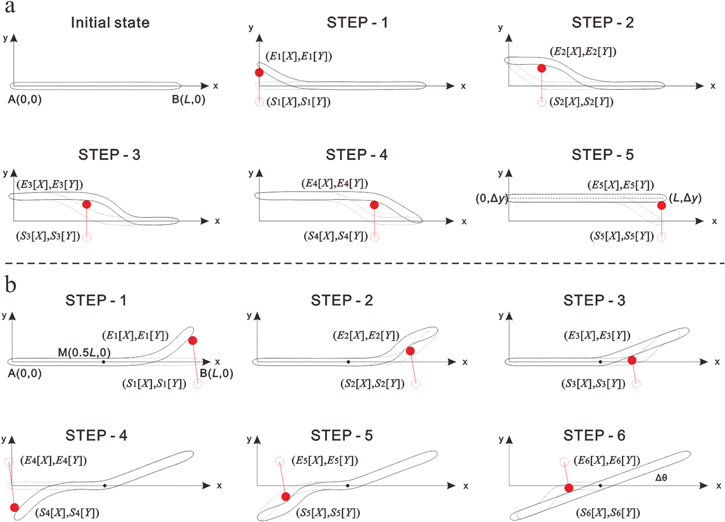
Figure 3. Schematic illustrations of (a) the translation and (b) the rotation strategies using PPVs. The empty and solid circles in each step represent the start and end positions of the AFM tip, respectively. The profiles of the NW in the dotted line and solid line represent the positions before and after manipulation, respectively. The pivot point M in (b) is the mid-point of the NW.
Download figure:
Standard image High-resolution imageThe rotation strategy is quite similar to the translation. The difference is that the lengths of these PPVs are not identical. In a former paper, we demonstrated that a single pushing vector rotates a rigid nanotube around a pivot point [20]. Here we also suppose that a pivot point exists on the flexible NW. The length of each vector is proportional to the distance between the force application point and the pivot point, and the direction of the vector points from the application point to the corresponding point on the target straight line.
Figure 3(b) schematically illustrates the PPVs for rotation, in which the pivot is located at the mid-point of the Ag NW. The pushing vectors applied to the two sides of the Ag NW are symmetrical about the pivot point. In the case of a small angle rotation, the coordinates of the start point and the end point of the nth vector are determined by the following equations:
In the above equations, Δθ is the rotation angle, and the other parameters have the same meaning as in equation (5). For either half of the Ag NW, the pushing vectors located further from the pivot are executed with higher priority. This is because the NW is easier to rotate from the ends. Like the process of translation, the whole NW is expected to achieve the target direction and be re-straightened when all the vectors are completed. By accumulating small angle rotation the larger angle rotation can be realized.
Though in figure 3(b) the Ag NW is supposed to rotate around its mid-point, the pivot may actually be in another position on a flexible sample, especially when it is very soft. We prefer to use the mid-point because in this case the total length of the PPVs reaches a minimum and hence the rotation process is more efficient. But if the NW has a large amount of bending stiffness, the mid-point is perhaps not a reasonable choice. Let us consider the extreme condition, in which the NW is rigid, and the pivot point is then uniquely determined by the self-balance equations [20]. If the pushing force is applied to B(L, 0), the pivot will be located around the point R(0.3L, 0). The R point is also a possible pivot for those NWs that are stiff but still flexible, and in this case the PPVs are determined as follows:
It should be noted that there is not a clearly defined border between the stiff and soft NWs. In principle, an NW with large thickness and elastic modulus has high bending stiffness, but it may still behave like a soft wire if it is long enough or the friction is extremely strong. In most cases, the modulus and the friction are not precisely measured, so the selection of the pivot is somewhat empirical. A simple push test would help to find the proper model.
2.3. FEM simulation
Although the behaviour of the Ag NW under a single push manipulation can be described using equations (1)–(4), we found it was difficult to give a precise analytical expression of the final state of the NW after multiple pushing. Instead of a formulation, the simulation based on a finite element method (FEM) was used to investigate the effects of the present strategies and to guide the parameter selection for the PPVs. The simulation was performed using ANSYS. The Ag NW model in the simulation was a 2 μm long prism with a pentagon cross section. It was laid on a flat hard substrate with one of its faces in contact with the substrate surface. The height of the NW, i.e. the distance from the bottom face to the upper ridge, was 50 nm. The density and the Poisson ratio were 10.5 ×10³ kg m−3 and 0.38. The elastic modulus was 80 ∼ 120 GPa according to the early literature [25]. A pressure of 0.5 ×10⁸ Pa was added to the NW substrate contact area in order to generate friction. The dynamic friction per unit length was given by q = 0.65 P · h · μd, where μd represents the dynamic friction coefficient, which is half the static friction coefficient. In this simulation, μd varied between 0.05 ∼ 0.2, so the dynamic friction and the maximum static friction were respectively in the range of 0.12 ∼ 0.5 nN nm−1 and 0.2 ∼ 1.0 nN nm−1, which is consistent with our direct measurement result (see supporting data is available online at stacks.iop.org/NANO/28/365301/mmedia). The AFM tip was modelled as a silicon hemisphere with a radius of 35 nm. The pushing vectors were sequentially applied to a series of evenly spaced positions along the Ag NW through the displacement of the tip. The interval of these vectors, i.e. Δx, was 150 ∼ 600 nm. The displacement of each step in the translation, i.e. Δy, was 50 ∼ 200 nm. The rotation angle Δθ was 3 ∼ 5°.
Figure 4 displays a typical translation simulation result, in which E = 80 GPa, μd = 0.2 (i.e. q = 0.5 nN nm−1), Δx = 321 nm and Δy = 100 nm. As seen in the figure, the parallel pushing strategy resulted in the wriggling behaviour of the Ag NW. In each step, a small part of the NW around the force application point was moved 100 nm forward. When all seven pushing steps were completed, the whole body of the NW was on the target line. Although this NW still appeared to be slightly curved after the last pushing step, the straightness was apparently improved compared to the intermediate steps. The maximum stress introduced by this manipulation was about 1.8 GPa, occurring at the most curved point in the sixth step. After the last pushing step, the residual stress significantly decreased. In most regions, the residual stress was below 0.3 GPa. The residual stress was due to local deformation of the NW during movement. If the inner tensile force is not able to overcome the static friction, the deformation cannot be released. A smaller Δx and Δy would help to reduce the residual stress.
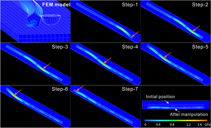
Figure 4. An FEM simulation of the translation strategy. Seven PPVs (red arrows) of equal length and intervals were sequentially applied to the NW along its longitudinal direction. The top left image shows the FEM models of the Ag NW and the AFM tip. The bottom right image is a top view of the initial and final states of the sample. The NW was finally moved 100 nm to the target position. The colour bar indicates the stress distribution in the NW.
Download figure:
Standard image High-resolution imageFigure 5 displays two typical simulation results of rotation around the mid-point and the R-point. In this simulation, Δθ = 5°, Δx = 400 nm and E and μd are the same as in figure 4. The maximum bending stress introduced by rotation always occurred in the first step. The peak value was about 1.3 GPa when the NW was rotated around the mid-point. When the pivot shifted to R, the lever arm from the first pushing vector to the pivot was extended. Thus, the deflection of the NW in the first step grew larger, which increased the maximum bending stress to 1.6 GPa. After the last manipulation step in both the upper and lower images, the Ag NW was successfully turned in the expected direction with an almost straight shape. The residual stresses were 0 ∼ 0.8 GPa and 0 ∼ 0.6 GPa, respectively.
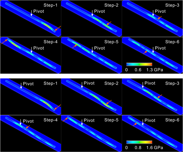
Figure 5. An FEM simulation of the rotation strategy. The pivot points in the upper and lower images, respectively, located at the mid-point and the R-point of the Ag NW. Six PPVs (red arrows) of proportional length and identical intervals were sequentially applied to the NW from the ends to the pivot. The angle between the initial position and final position was 5°; the colour bar indicates the stress distribution.
Download figure:
Standard image High-resolution imageFrom a series of simulations with different E, μd, Δx, Δy and Δθ, we learnt that all these parameters had a significant influence on the final state of the NW. With a higher modulus and lower friction, the NW will have a smoother shape after manipulation, because in this case the same deflection drives a longer segment of the NW to be bent. This is also in agreement with the analysis for a single push, as illustrated in figure 1. However, the final straightness could be worse due to the increased possibility of rebounding. Rebounding can occur in a wide region around the force application point, and the rebounding parts can stop in unpredictable positions. In comparison, soft NWs are more controllable, as each part of the NW can be directly moved to the target position and held stably by the static friction. High amounts of friction on the substrate help to maintain the shape and position of the NW, but on the other hand, it also makes movement difficult. The NWs are more likely to be broken, and the higher residual stress will cause them to become unstable.
For a given modulus and friction properties, shorter vectors and smaller intervals ensure lower amounts of stress as well as better straightness. Nevertheless, it requires more steps to transfer the NW over the same distance, and hence the time consumption increases. Therefore, a trade-off must be made between the manipulation efficiency and the final straightness of the sample. Two principles for selecting Δx, Δy and Δθ are as follows:
- 1.The maximum stress caused by Δy or Δθ must be lower than the yield strength of the material;
- 2.Δx must be no more than half the length of the curved segment caused by a single pushing vector.
In the simulations shown in figures 4 and 5, the maximum stresses are 1 ∼ 2 GPa, which are close to the reported yield strength of Ag NWs [26–28]. Thus 100 nm and 5° can be taken as the upper limits of Δy and Δθ under the related conditions. Nevertheless, because the maximum friction coefficient measurement is used in this simulation, Δy and Δθ are allowed to be a few times larger in the experiment. According to equation (3), the length of the curved segment is about 10 times that of Δy; thus Δx should be smaller than 5Δy.
In our simulation, no rolling behaviour was observed. Although there was a twisting trend when the first pushing vector was applied to the end of the NW, the torque induced by the AFM probe was insufficient to encounter adhesion on the substrate surface. Sliding is the only form of motion that should be considered in this strategy.
3. Experiments
A series of manipulation experiments were carried out to confirm the efficiency of the presented strategies. The Ag NWs used in the experiments were produced by Blue Nano Inc., Jinan, China. We dispersed the Ag NWs in ethanol with a density of 1 mg ml−1 following 20 s ultrasonication. Then a droplet of the suspension was deposited on a silicon dioxide substrate and dried in air at room temperature. The humidity ranged within 32% ∼ 35% during manipulation. From the AFM measurement, the roughness of the substrate surface was less than 0.3 nm (Rq), and the thickness and the length of the Ag NWs were in the range 25 ∼ 80 nm and 2 ∼ 15 μm, respectively.
All the characterization and manipulation was conducted with a commercial AFM platform (Dimension ICON, Bruker) combined with a MATLAB program particularly designed for the manipulation task. The AFM was operated in tapping mode in air for the image scan. Once an image had been captured, the raw image file was loaded into the MATLAB program. Through the graphic user interface, the users can select the NW and specify a target position in the image area. Then the MATLAB program automatically generates the manipulation paths based on the corresponding strategies, and saves the coordinates of all the vectors as well as the other manipulation settings (e.g. the movement velocity of the probe) into a text file. Because the NWs are randomly distributed in the image area, the coordinate transformation must be made before generating the manipulation vectors. In the image coordinate system (xoy system), supposing the coordinates of the A end of the Ag NW are (x0, y0), and the orientation angle of this NW is α, then the coordinates of all the vectors given by equations (5)–(7) must be converted using the following equation:
Once the path file has been successfully generated, the AFM system reads out the corresponding information from the text file, and drives the scanner to sequentially execute all the manipulation actions. When a pushing vector is in processing, the feedback in the z-direction is temporarily turned off, and the probe slides on the substrate with a preset vertical press. This vertical press is usually a few tens to hundreds of nano-Newtons, which prevents the probe from climbing over the sample. The cantilever probes used in this experiment were NSG01 manufactured by NT-MDT with a rectangular cantilever. According to our measurement using a traceable calibration system [29], the effective spring constants of this cantilever in the normal and lateral directions are 8.32 N m−1 and 99.37 N m−1, respectively. The nominal value of the tip radius is 12 nm.
4. Results and discussion
Figure 6 shows a translation experiment; in this image area, two Ag NWs can be found. The one near the centre of the image is selected as the manipulation object while the other NW is considered as a static reference. The selected Ag NW is about 45 nm in height and 2.1 μm in length. From figure 6(a), we obtained the initial coordinates of the NW and then specified a target line 0.33 μm in front of it. Five PPVs were generated based on equations (5) and (8) for the translation. To confirm the intermediate state of the NW, images were captured after every single vector. As shown in figures 6(b)–(f), the NW wriggles forwards in steps and finally achieves the target line with a well-straightened configuration. A small burl can be seen near one end of this NW. Throughout the process this burl remains along the same lateral line as the NW, indicating that no rolling has happened during the translation. This result is in agreement with the simulation.
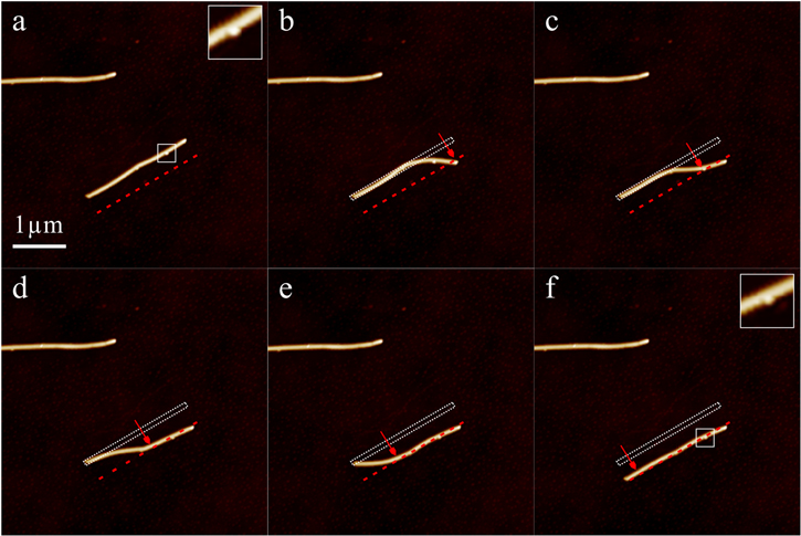
Figure 6. Experiment translating a straight Ag NW. The red dashed lines represent the specified target position; the arrows represent the PPVs. In images (b)–(f) the initial position of the NW is marked by a dotted bar. The insets in images (a) and (f) show the zoomed burl feature on the NW.
Download figure:
Standard image High-resolution imageFigure 7 presents the rotation experiment of the same NW as in figure 6. Six PPVs generated using equations (6) and (8) were applied to rotate the NW around its middle. To make the rotation result more visible, a large angle of about 25° was assigned in this experiment. As seen in the images, the NW was rotated in the target direction and re-straightened after the last step. Compared to the other steps, the shape of the NW changed little in the 3rd and the 6th steps. This is because the two pushing vectors were very close to the pivot point, and thus the vector length was too short. Since the pushing vectors near the pivot did not contribute much to the final shape, it was possible to leave them out, reducing the time consumption in practice. The insets in figures 7(a) and (f) indicate that the NW did not roll axially when it was rotated around the pivot in the plane. Sliding was always the prior motion, both in translation and rotation. Although in this experiment the NW was successfully turned by 25° with only one round of parallel pushing, we still suggest using a small angle of rotation each time for better stability.

Figure 7. Experiment rotating the same Ag NW, as shown in figure 6. The final position achieved in figure 6(f) is the initial position in this experiment. The pivot is located in the middle. All the symbols in this figure have the same meaning as those in figure 6. The insets in (a) and (f) prove that the burl remains at the same lateral position of the NW during this rotation.
Download figure:
Standard image High-resolution imageIn the above we have demonstrated the translation and rotation strategies for straight Ag NWs. However, the initial configuration of the Ag NWs may not simply be straight after they have been dispersed onto the substrate. In this case, additional straightening manipulation must be performed before translating or rotating the samples. In our experiment, the most typical shape of the flexed Ag NWs is that of multi-section cudgels. That is, the Ag NWs are divided into a couple of straight sections by several linked joints. We applied the rotation strategy again to straighten these samples. The idea was to rotate each section around the joint till the angle between the two adjacent sections reached 180°. An example is presented in figure 8. The flexed Ag NW shown in figure 8(a) is about 75 nm thick and 4 μm long. Its initial configuration consisted of two equal-length straight sections, with an angle between them of about 140°. The original AFM image was then loaded into the MATLAB program, and one of the two sections was selected to be rotated around the joint, as seen in figure 8(b). Six PPVs were applied as a group, rotating the manipulated section by 1° each time. After 40 rotations, the whole NW was unfolded into a straight line as shown in figure 8(c). Though a slight inflexion can still be observed around the joint, it does not affect the subsequent application of the translation and rotation strategies.

Figure 8. Experiment straightening a flexed Ag NW. (a) and (c) The initial and final state of the Ag NW; (b) the generation of the target and pushing vectors in MATLAB.
Download figure:
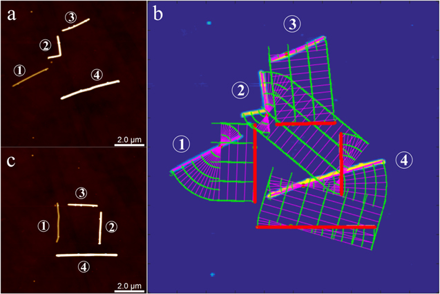
Standard image High-resolution imageSince we were already able to precisely translate and rotate the individual Ag NWs to the specified positions, it became possible to continuously manipulate multiple Ag NWs to form patterns on the substrate. Figure 9 gives an example of the assembly of a simple rectangular pattern of Ag NWs. Figure 9(a) shows a 10 μm × 10 μm area, where four Ag NWs with different dimensions are randomly dispersed. The thickness and lengths of them were within 35 ∼ 75 nm and 2.7 ∼ 4.2 μm, respectively. All these Ag NWs were initially straight except NW no. 2, which flexed like a flipped letter 'L'. The image data was processed using the MATLAB program, as shown in figure 9(b). We assigned target positions for each NW through the graphic user interface, and then the MATLAB program automatically generated all the PPVs based on the strategies introduced previously. The manipulation priority of these NWs was ④-③-②-①. The order is important for the manipulation of multiple objects, since they are probably barriers to movement on each other's paths. We used graph theory to determine the sorting, the detail of which will be discussed elsewhere. The manipulation procedure for each NW was similar. The NW was firstly straightened if necessary, and in this experiment, only NW no. 2 undertook straightening manipulation. Then the NW was rotated around the pivot until it was perpendicular to the line joining the same pivot points at the initial position and the target position. In the next step, the NW was translated towards the target position until the distance between the pivot points was smaller than a threshold (50 nm in this case). Finally, the NW was rotated around the selected pivot point again if necessary to fit the target orientation. In this experiment, the R-points were selected as the pivots for all four Ag NWs. The minimum rotation angle in each step was 5°. For NW no. 4, eleven PPVs were applied as a group for rotation, and seven PPVs were applied as a group for translation. It was first rotated by 35° clockwise and then translated over 1.2 μm to the target, and finally rotated again by 15° counter-clockwise. For NW no. 2, it was straightened first, and three PPVs were employed as a group to rotate the shorter section by 90° around the joint. After being straightened, the NW was rotated 45° clockwise, then translated by about 3 μm, and finally rotated 40° counter-clockwise. Here, six and four PPVs were respectively set as the pushing vector group for rotation and translation. For NW no. 1, the seven PPV group and the five PPV group were respectively employed for rotation and translation. The wire was first rotated 60° counter-clockwise and then translated by about 1 μm to overlap the target line directly. For NW no. 3, the six PPV group and the four PPV group were respectively used for rotation and translation. The wire was first rotated 15° clockwise and then translated by about 2.5 μm, and finally rotated 5° clockwise again. It can be seen in figure 8(c) that the final shape and positions of all four Ag NWs is well consistent with the pattern defined in figure 8(b). This manipulation included more than 460 PPVs. All of them were processed continuously and automatically without interruption by image scanning. The whole assembly was completed within one hour, which is much faster than the conventional way. If a high-speed AFM scanner is used, the time consumption will hopefully decrease to a matter of minutes.
Figure 9. The nanopattern assembly using multiple Ag NWs. (a) and (c) The positions of the four Ag NWs before and after manipulation. (b) The automated image processing and PPVs generated by the MATLAB program. The straight red lines represent the specified target positions of the NWs. The straight pink lines represent the initial positions (thicker lines) and the predicted intermediate positions (thinner lines) of the NWs. The green lines represent all the pushing vectors.
Download figure:
Standard image High-resolution image
5. Conclusions
In conclusion, we have reported new strategies for the manipulation of flexible Ag NWs. Mechanical modelling and FEM simulations were carried out to analyse the behaviour of the sample and optimize the manipulation method. By using PPVs, we were able to straighten, translate and rotate individual Ag NWs with a precisely controlled configuration and position. The present strategies, as well as the new manipulation technique, make it possible to realize the automatic assembly of nanopatterns. The present strategies may also be applied to other nonrigid NWs with a simple adjustment of the manipulation parameters. This study will help to increase the efficiency of AFM-based manipulation and benefit the fabrication of molecular devices.
Acknowledgments
This research is supported by funds from The National Natural Science Foundation of China (61204117, 61633012 and 51675379).