
Abstract
While piezoelectric energy harvesting typically focuses on converting mechanical into electrical energy on the basis of the linear reversible piezoelectric effect, the potential of exploiting the non-linear ferroelectric effect is investigated theoretically in this paper. Due to its dissipative nature, domain switching, on the one hand, is basically avoided in order to prevent mechanical energy from being converted into heat. However, the electrical output, on the other hand, is augmented due to the increased change of electric displacement. In view of these conflicting issues, one main objective in ferroelectric energy harvesting thus is to identify mechanical and electrical process parameters providing appropriate figures of merit. Being an efficient approach to numerically simulate multiphysical polycrystalline material behavior, the so-called condensed method is taken as a basis for the investigation and finally optimization of controllable parameters of ferroelectric energy harvesting cycles. A first idea of a technical implementation taken from literature is considered as cycle of reference, constituting the starting point of the present study, being focused on material aspects rather than on harvesting devices. Different quality assessing parameters are introduced, taking into account general aspects of harvesting efficiency as well as the ratio of irreversible switching-related to reversible piezoelectric contributions. Residual stresses are likewise predicted to give an idea of reliability and the risk of fracture. Two types of cycles and associated optimal process parameters are finally presented.
Export citation and abstract BibTeX RIS

Original content from this work may be used under the terms of the Creative Commons Attribution 4.0 license. Any further distribution of this work must maintain attribution to the author(s) and the title of the work, journal citation and DOI.
1. Introduction
Avoiding the dispensable usage of eco-unfriendly and costly batteries, energy harvesting exploiting ambient energy sources has been widely explored in recent decades. Aside from thermal energy, vibration sources have been of particular interest due to their common and manifold occurrence in nature [1]. As a result of experimental research and numerical simulations, various energy harvesting concepts for conversion of mechanical to electrical energy have been proposed [2–4]. Due to their suitable electromechanical properties, piezoelectric materials have been thoroughly investigated in this context [5–8]. Such harvesting devices commonly consist of piezoelectric layers attached to vibrating structural components. The main difficulty researchers have encountered is the strong dependence of output and efficiency on the harvester's resonance frequency, which is commonly not met by the ambient vibration source, usually exhibiting a rather broad bandwidth [9]. Thus, attempts were made to improve the efficiency by adapting the harvester's range of effective performance [10, 11]. In light of this, non-linear energy harvesting systems in terms of either geometrical or physical non-linearity have been explored [12–14]. Ferroelectrics could potentially generate a larger energy output than conventional piezoelectrics, since their unit cells are able to perform a discrete and thus non-linear change in shape and polarization if sufficiently loaded electrically or mechanically. Exploiting just the linear reversible effect, changes of polarization in piezoelectric energy harvesting are comparatively small and restricted to the magnitude of the dipole moment, directly controlled by elastic strain input. Ferroelectric harvesting concepts, on the other hand, exploit the much larger amount of polarization changes due to domain switching and thus rotation of the dipole axes, finally leading to an augmented electric work output being independent of resonance frequencies and modes of vibration.
A small number of concepts exploiting these effects, known as ferroelectric and ferroelastic switching, respectively, in regard to energy harvesting applications have recently been investigated theoretically [15–19]. Patel et al [15] propose a harvesting concept based on ferroelectric/-elastic domain switching in the rhombohedral phase of an antiferroelectric material, where compressive stress is applied for depolarization during the harvesting process and repolarization is achieved by electric loading. The output of electric work for different stress and electric field levels is assessed from hysteresis loops of polarization vs electric field measured for polycrystalline Pb0.99Nb0.02 [(Zr0.57Sn0.43)0.94Ti0.06]0.98O3 (PNZST) bulk ceramic under uniaxial or radial constant mechanical loading. In [16] polarization switching is suggested to be effectuated by a periodic sequence of compressive and tensile stress being in phase with a cyclic electric voltage to extract electrical work. This approach, however, requires a specific domain pattern e.g. prevailing in nano-domain single crystals. The feasibility of the concept is investigated in [16] by the phase field method. Wang et al [17, 18] first introduce a bias electric field supporting the polarization process in two different concepts with plate or interdigitated electrodes. While the plate electrode concept takes its energy for polarization essentially from compressive stress, the bias field provides this energy in the interdigitated prototype. The latter concept does not rely on tensile stress for depolarization, however requires a specific arrangement of electrodes. A harvesting electric field is not separately introduced in either of the concepts. The phase field method is applied to investigate influencing factors numerically, based on a poly-domain single crystal model.
Kang and Huber [19] put forth a quasi-static energy harvesting cycle suitable for polycrystalline ferroelectrics. The working cycle does not require any specific microstructure or electrode arrangement and exploits stress-driven de- and repolarization of the material via ferroelastic switching. Respective harvesting and bias electric loading during the phases of de- and repolarization serve either as resistance against which electrical work is done or as support to make sure unit cells switch back to their initial direction. Numerical simulations presented in [19] are based on a simple domain switching model and support the fundamental functionality of the concept which is depicted schematically in figure 1. The cycle starts at point A, where the material is pre-polarized, indicated by the red arrows. An external tensile stress σ11 effectuates a depolarization which, in connection with an electric harvesting field in x3 direction, delivers an output of electrical work  . From points B to C both the mechanical stress and the electric load are relaxed, leaving a depolarized remanent domain pattern. Subsequently, an input of both mechanical and electric works, mediated by lateral compressive stress σ11 and an electric field E3, respectively, leads to state D, whereupon the comparatively small electric bias field gives rise to a polarization in x3 direction. Relaxation of all external loads finally closes the cycle in point A. The electric benefit of the harvesting cycle thus is obtained in stage A–B, whereas mechanical work is inserted in stages A–B and C–D.

Figure 1. Schematic of one harvesting cycle exploiting ferroelectric and ferroelastic effects starting in a polarized state at point A.
Download figure:
Standard image High-resolution imageWhile figure 1 illustrates the ferroelectric harvesting idea from the material's perspective, a tangible engineering implementation inspired by [19] is demonstrated in figure 2. The required tensile and compressives stresses are accomplished attaching the ferroelectric to a cantilever device whose bending mode stores and provides the mechanical energy. Free charge  is periodically generated at the electrode due to repeated changes of the orientation of the electric dipole moment. Compared to a classical piezoelectric harvesting concept with constant polarization direction the only added complexity is provided by external control of voltages. On the other hand, the magnitude of electric energy output is considerably augmented due to the larger change of spontaneous polarization. A further advantage could be the use of comparatively thin layers based on the fact that the electrical and mechanical operating directions are perpendicular to one another.
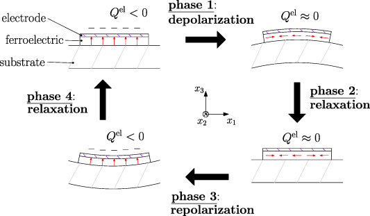
Figure 2. Engineering implementation of the ferroelectric energy harvesting concept based on a cantilever substrate.
Download figure:
Standard image High-resolution imageThis paper adopts the idea of a ferroelectric energy harvesting concept according to [19], numerically investigates a variety of influencing factors on the efficiency, develops prospects for an improvement of the process management and provides an upper bound of figures of merit by non-linear optimization. The condensed method (CM), which is used for the simulations, incorporates multiple aspects of polycrystalline ferroelectrics on different scales [20–22], thus allowing a more sophisticated theoretical analysis of the harvesting concept compared to previous work. In section 2.4 a brief overview on some basics of the CM is presented following an introduction to the theoretical framework of ferroelectrics including the microphysical constitutive model. Basics of the analysis and optimization of energy harvesting cycles are introduced in sections 2.5 and 2.6, respectively. The presentation of results starts in section 3.1 with the numerical analysis of the harvesting cycle introduced in [19], which will be denoted as cycle of reference (COR), including the suggested process parameters in terms of magnitudes of mechanical re- and depolarizing stresses as well as bias and harvesting fields. The evolution of strain as well as electric displacement and polarization, respectively, are calculated, just as pre-defined measures of functionality and efficiency. The latter issues being the basis of deeper analysis, a theoretical idealized cycle is identified, providing the best possible figures of merit. Residual stresses induced by domain switching are also predicted for the COR in order to obtain an idea of impacts on durability. Investigations of improvement potential of the efficiency in section 3.2 target both material-related quantities of ferroelectricity, in particular coercive field, spontaneous polarization and strain, as well as process parameters of the cycle. In section 3.3 an optimization will provide process parameters of a four parameter cycle akin to the COR and a six parameter cycle. Conclusions are finally drawn in section 4.
2. Theoretical framework
2.1. Fundamentals of irreversible quasistatic thermoelectromechanics
The balance equations of momentum and charge are given by


with the mass density ρ, the displacements ui
, the tensor of Cauchy stresses σij
, the volume forces bi
, the electric displacement Di
and the volume specific charge density  . Analytical notation is applied here as in the following, without distinguishing co– and contra–variant tensors, since only Euclidean coordinates are employed. Einstein's summation convention is applied to repeated indices, while the number of single indices indicates the order of the tensor. A comma denotes a spatial partial derivative, a dot indicates a time derivative. Volume related quantities are represented by lowercase letters, whereas capital letters are employed for the associated absolute and extensive state variables. Current and reference configurations are further not distinguished due to geometrical linearity of the model. In the following, bi
and
. Analytical notation is applied here as in the following, without distinguishing co– and contra–variant tensors, since only Euclidean coordinates are employed. Einstein's summation convention is applied to repeated indices, while the number of single indices indicates the order of the tensor. A comma denotes a spatial partial derivative, a dot indicates a time derivative. Volume related quantities are represented by lowercase letters, whereas capital letters are employed for the associated absolute and extensive state variables. Current and reference configurations are further not distinguished due to geometrical linearity of the model. In the following, bi
and  are assumed to be zero in a dielectric material and mass inertia is neglected in the quasistatic limit, i.e.
  .
.
Based on the internal energy  , as thermodynamical potential, with strain
  , electric displacement and entropy S as independent variables, the corresponding Gibbs fundamental equation of the specific potential is obtained as

Ei
denotes the electric field and T the absolute thermodynamic temperature. Furthermore,  and
and  are the reversible contributions of mechanical strain and electric displacement, respectively, which can be classically decomposed according to
where  and
and  denote the irreversible strain and polarization, respectively. The entropy rate being composed of an irreversible part
  due to dissipation and an exchange part
  due to heat transfer, i.e.

and the dissipation rate  being related to specific dissipative electrical and mechanical works according to
where  denotes the specific irreversible work rate in a volume V, equation (3) can be rewritten as
where the mechanical and electrical works are identified as  and
and  , respectively. Equation (7) will play a crucial role in the analysis of harvesting cycles, see section 2.5. The heat rate includes the volume heat source
  and the heat flux across the boundary
  , i.e.
where Gauss' integral theorem has been applied. The 2nd law of thermodynamics postulates
Inserting equations (5), (6) and (8) and neglecting  , the generalized Clausius–Duhem inequality is obtained as
whereat the second term (including the sign) is always positive. Equation (10) is essential to prove the thermodynamic consistency of the evolution equations of internal variables which will be introduced in section 2.3.
2.2. Constitutive equations of ferroelectricity
Restricting simulations to electro–mechanical issues, the caloric quantities, i.e. temperature and entropy, will be disregarded subsequently. Dissipation, being a crucial aspect of the numerical investigations, still prevails in the model, however, impacts on temperature and heat flux are thus not considered. The electromechanical thermodynamical potential of ferroelectrics is postulated as follows
Obviously, the independent variables are different from those of the internal energy density  , which results from a Legendre–transformation, replacing the electric displacement by an electric field as independent variable. In equation (11)
  are the tangent moduli of elasticity, dielectricity and piezoelectricity. Furthermore, equation (11) depends implicitly on internal variables describing domain switching, and appearing in the tangent moduli as well as the irreversible quantities introduced in equation (4). The associated variables are obtained from equation (11) by differentiation with respect to the independent variables:
Coming up with the total differentials of stresses and electric displacements, these relations are applied to incremental changes of state if tangent moduli  , as second partial derivatives of ψ, are taken constant in each increment, finally yielding the rate–dependent formulation of the constitutive equations of ferroelectricity:


Differentiation of the potential from equation (11) with respect to an arbitrary internal variable ν(n), where the superscript n could refer to any ferroelectric domain being in a switching condition, provides the negative thermodynamic driving force
being equal to the specific dissipation Δχ(n), associated with switching of a domain n, see equation (6). The total specific irreversible work rate  of an entity of N switching domains, representing a dissipation potential, is obtained as
where equation (15) has been taken into account. Finally, equation (16) and the potential according to equation (11) satisfy the closure condition of thermodynamic consistency [21]
2.3. Microphysical model of ferroelectric domain switching
Figure 3 shows schematically the domain structure of a plane tetragonal ferroelectric grain. In the right sketch, a planar and a spatial grain are represented by single material points with four and six polarization directions, respectively. Adopting an idea from [23], the domain structure of a grain is transferred into the model by introducing internal variables ν(n) ∈ [0, 1] weighting the volume fractions of the domains n and satisfying the conservation condition
with n ∈ {1, ..., N} and N being the number of prevailing polarization directions. In this work, N = 6 is chosen, representing a 3D domain structure. Obviously, identical volume fractions for all domains represent an unpolarized state with the condition  . Bridging the levels of domain and grain, the weighted sums of material properties ϕ(n) of all domains are introduced [24] according to
where

The coefficients of the ϕ(n) thus represent single domain single crystals, however, being scarcely available [25]. In simulations based on microphysically motivated models of ferroelectric or other domain–structured materials [23, 25–28], polycrystalline properties are thus commonly employed at this point whereupon equation (19) still averages the different orientations of transverse isotropy in a grain. The rate–dependent irreversible strain and polarization due to domain wall motions are likewise modelled as weighted sums, now with rate–dependent internal variables, i.e.
where  specifies the spontaneous strain in tetragonal unit cells due to 90∘ switching and
  is the change of spontaneous polarization for transition from domain species (A) to species (B) [24]. In equation (21) only negative rates
  are considered, corresponding to donating and decreased domain species, respectively. Furthermore, the latter equation yields another representation of the thermodynamic driving force according to equation (15), reading

Equation (22) implies that σij and Ei remain constant during switching, arising from equation (15) where material coefficients just as stress and electric field have been assumed to remain incrementally unchanged. Considering equations (16), (21) and (22) the dissipative power at grain level is finally obtained as
The intuitive formulation of equation (6) is thus confirmed at this point. The evolution equations of internal variables are given by
where  denotes the Heaviside function, taking values 0 or 1 and
  is a model parameter which has been chosen equal for all domain species. It represents an arbitrary quantum of domain wall motion per calculation step, which has to be chosen within a context of competing time efficiency and numerical stability. The dissipative work
  of switching according to equation (22), is the maximum going along with all possible variants for the domain type n, associated with the favored species
  . Thus, the species n is the source being reduced in favor of the target
  if
if  . For tetragonal unit cells in each domain, the possible changes of state in terms of switching are β = 90∘ in two perpendicular planes and β = 180∘. The dissipative work has to overcome a critical value or an energy barrier
  , depending on the change of state β, to reduce the volume fraction of the concerned species by d
 . The favored species
  is then enriched by the same volume fraction, thus guaranteeing the conservation of volume for the entity of domains, see equation (18). The energy barriers are given as [28]
The evolution equation equation (24) is thermodynamically consistent, satisfying the Clausius–Duhem inequality equation (10), accounting for equation (23).
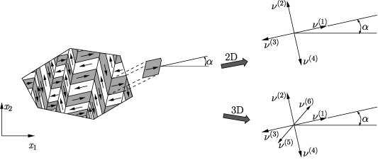
Figure 3. Two dimensional depiction of a tetragonal domain structure of a grain (left) with orientation α in global coordinate system  and representation by internal variables ν(n) in 2D and 3D models.
Download figure:
Standard image High-resolution image2.4. Condensed method for meso–macro transition
Macroscopic quantities in a polycrystalline representative volume element (RVE) are obtained by volume averaging stress and electric displacement according to
where m ∈ {1, ..., M} labels the grains, being assumed to hold identical sizes [20]. In equation (26) angeled brackets denote volume averaged macroscopic quantities and the superscript (m) refers to the quantities on the grain level, where the constitutive equations


hold in the style of equations (13) and (14). For the quantities not averaged according to equation (26), a generalized Voigt approximation is introduced, whereupon strain and electric field are assumed to be homogeneous in a RVE and thus equal in each grain:
Other approximations, i.e. Reuss or mixed Voigt–Reuss, are basically possible. The advantage of the choice of equations (29) is that residual stresses  due to grain interaction are directly provided. The choice of homogeneous variables is going along with the appropriate choice of independent variables in a thermodynamical potential, see equation (11), however has no impact on the choice of Dirichlet or Neumann type boundary conditions.
To obtain the macroscopic constitutive equations of a RVE, equation (26) is applied to the equations (27) and (28) while equations (29) and (30) are taken into account, resulting in


where e.g.
with  and
and  being determined from equations (19) with ϕ = Cijkl
and (21) for each grain. The balance equations (1) and (2) of linear momentum and charge are intrinsically satisfied inserting the averaged quantities according to equations (31) and (32). Consequently, e.g. for pure electrical loading,
being determined from equations (19) with ϕ = Cijkl
and (21) for each grain. The balance equations (1) and (2) of linear momentum and charge are intrinsically satisfied inserting the averaged quantities according to equations (31) and (32). Consequently, e.g. for pure electrical loading,  holds for average stresses in the RVE [20]. The residual stresses
  due to grain interactions in an electric field
  are determined from equation (27), inserting the macroscopic strain

which has been derived from equation (31):
In equations (34) and (35) the external mechanical load has been introduced as  . The macroscopic electric displacement is derived from equations (32) and (34):
For more details concerning the CM we refer to recent works, e.g. [21, 22].
2.5. Analysis of energy harvesting cycles
In order to simulate the ferroelectric energy harvesting cycle with the CM, macroscopic mechanical stresses and electric fields are stipulated external variables marked with 'ext' or set to zero where applicable, in Voigt-notation reading


Equations (37) and (38) illustrate the uniaxial stress and electric field loadings in the x1 and x3 directions, respectively, as depicted in figure 1. Strains and macroscopic electric displacements are unknowns to be calculated from equations (34) and (36):

In the following, N will denote the current load step,  the amount of load steps per loading cycle, and
  the number of load cycles. Furthermore, the subscript 'lc' will indicate a quantity in respect of one load cycle. In order to determine the electrical and mechanical works that are done during one load cycle, the total differential of the volume specific internal energy is considered according to equation (7). In a stationary cycle, each of the independent variables holds identical magnitudes at the starting and the final load steps, i.e.
  . The same should hold for the internal variables ν(n), the corresponding associated variables, i.e.
  , as well as for the specific internal energy u. Integrating equation (7) in the limits
  and
and  consequently leads to
where  is the specific heat flux of one cycle. The dissipation related entropy is included in the specific works, thus not depicted explicitly. Accordingly, the electrical work of one load cycle is identified as
whereas the mechanical work is defined as
By decomposing the electromechanical works into reversible and irreversible parts in analogy to strains and electric displacements in equation (4), the contributions of the reversible piezoelectric effect and the irreversible ferroelectric effect are distinguished:
The reversible and piezoelectric, respectively, parts of electrical and mechanical works being entirely converted into one another, given that the changes of material properties due to domain wall motion are negligible, i.e.

Equations (41) and (44) lead to

Equation (46) illustrates that irreversible mechanical and electrical works of one load cycle are dissimilar due to the heat flux which is indispensable to close a cycle in a dissipative process, here due to domain switching. Disregarding caloric aspects in the modeling at this point, three of the six electromechanical works in equation (44) are independent and remain to be calculated, while the other three are determined from equations (44) and (45). In the following,  and
and  will be the chosen ones emanating from the simulations of harvesting cycles. Applying volume averaging and Voigt approximation according to equations (26), (29) and (30), while considering electromechanical variables according to equations (37)–(40), the macroscopic electromechanical works are calculated by the CM via trapezoidal rule as follows:
Obviously only the x3 components of the electrical variables and the 11 components of the mechanical variables contribute to the electrical and mechanical works, respectively. Since conversion of mechanical to electrical work represents the fundamental purpose of energy harvesting, a cycle will be considered functional if the mechanical input is positive whereas the electrical output is negative, i.e.  and
and  . However, this necessary criterion is not sufficient for a comprehensive evaluation of the process since it could be satisfied solely exploiting the linear piezoelectric effect. Consequently, a sufficient functionality criterion postulates the irreversible electrical work to be contributing to the energy output, i.e.
  . In order to evaluate energy harvesting cycles in more detail including and beyond these criteria, three independent quality-assessing quantities are introduced as follows:
where η is the total efficiency,  is the degree of irreversibility and
  is the ferroelectric efficiency. While negative efficiencies η and
  correspond to nonfunctional and nonadequate cycles, respectively, the degree of irreversibility may basically take both signs for a functional cycle.
2.6. Optimization
Constrained non-linear optimization problems are generally constituted as follows:

In equation (51),  represents the target function,
  the input parameters,
  the inequality constraints and
  the equality constraints. The maximum of the target function is sought within the allowable range Z of the input parameters, which is given by

In our case, the inequality constraints are given e.g. by upper limits of values for the process parameters  , see figure 1, the latter constituting the input parameters
  . Equality constraints, on the other hand, do not apply and a target function could be the irreversible electric work output. Altogether, a global maximum
  and its maximum point
  have to satisfy the following criterion:

In order to approximate a solution, a single objective genetic algorithm, belonging to the class of evolutionary algorithms and exhibiting one single target function, is used [29]. Akin to evolutionary processes in nature, a population of 40 initially random sets of parameters  is repeatedly modified by recombination and mutation in order to identify the fittest set. The process is stopped as soon as the relative variation of the average value of the target function in the population remains below 0.1% within ten modifications. The algorithm is implemented into the open source code Dakota [30].
3. Results
Material data of barium titanate (BT) were taken from [20]. The irreversible polarization, however, has been reduced by 40% in the simulations, taking into account compensation by free charge. Spontaneous strain was likewise reduced by 15% to account for the fact that domains may not totally disappear. The number of grains per RVE was chosen M = 60, the amount of load steps per cycle  and the quantum of changed volume fractions of domains in the evolution equation equation (24)
  . First of all, the COR is analyzed with regard to polarization efficiency and related work flows and quality factors, stationarity as well as principle stresses. Subsequently, the influence of the ferroelectric material parameters on the COR is investigated, followed by the exploration of the process parameters. Finally, optimizations are carried out with respect to harvesting efficiency and in order to maximize the cycle's exploitation of the ferroelectric effect.
3.1. Cycle of reference (COR)
3.1.1. Process parameters and loading scheme.
The numerical simulations of the COR are realized by applying the electromechanical loading scheme illustrated in figure 4, with the points ① to ⑩ highlighting distinctive states of the cycle. In figure 4(a) the stress is normalized with respect to
Figure 1 illustrates the role of harvesting and bias electric fields as well as polarizing and depolarizing mechanical stresses in the ferroelectric harvesting concept, which in the COR have been selected as follows [19]:
During prepolarization (PP) between points ⓪ and ②, the material is polarized by applying an electric field sufficiently beyond  up to
up to  . At point ① the coercive electric field is reached, thus the first switching processes are initiated. The initial state of the energy harvesting cycle is marked by point ②. From ② to ③ in the first phase (P1), the constant harvesting field
  is applied into the x3 direction, while a linearly rising tensile stress up to
  in the x1 direction leads to 90∘ switching processes, depolarizing the material. Therefore, electrical work is obtained as charge is displaced against the harvesting field. In the second phase (P2), between the states ③ and ④, the electric field instantaneously drops to zero, while the stress load is kept constant. Subsequently, the material relaxes, as the tensile stress reduces to zero between points ④ and ⑤. The third phase (P3) is initiated applying a small bias field
  from points ⑤ and ⑥ aligned with the
  direction. Thereafter, a compressive stress in the x1 direction rises linearly up to
  in between ⑥ and ⑦, leading to 90∘ switching, due to the bias field mostly in positive x3 direction, thus repolarizing the material. Ultimately, in the fourth phase (P4), the electric field once again drops to zero from ⑦ to ⑧. By reducing the compressive stress to zero, the material relaxes from ⑧ to ⑨. In order to return to the initial state of the cycle, the harvesting field is once more applied into the x3 direction from ⑨ to ⑩, in contrast to the poling process ⓪–②, however, in the shape of a harsh jump. The corresponding results of calculation for strain
  and electric displacement
  are shown in figure 5.

Figure 4. Electromechanial loads of the cycle of reference; (a) normalized macroscopic stress  , (b) normalized electric field
  versus normalized steps
  of the first load cycle.
Download figure:
Standard image High-resolution image
Figure 5. Electromechanical variables of the cycle of reference resulting from the loading scheme in figure 4; (a) normalized macroscopic stress versus normalized macroscopic strain, (b) normalized macroscopic electric displacement versus normalized electric field.
Download figure:
Standard image High-resolution imageAccordingly, figure 5(a) shows the stipulated stress  plotted vs the calculated strain
  , while figure 5(b) shows the macroscopic electric displacement
  plotted vs the stipulated electric field
  . All quantities are normalized with respect to
  according to equation (54), the spontaneous strain
  or polarization
  , or the coercive field
  . In both plots, the process sequence is indicated by arrows. Apart from the prepolarization (PP) and the first cycle, the beginning of the second cycle is illustrated as well. In figure 5(b), the harvesting and depolarization of phase P1, respectively, proceed from states ② to ③, where the macroscopic irreversible polarization
  decreases, in turn leading to a decrease of
  . Analogously, an increase of
  takes place from points ⑥ to ⑦ due to the repolarization in phase P3. On the one hand, the blue areas within the plots of figure 5 represent the positive mechanical work
  and the positive electrical works
  and
and  , respectively, which are performed on the system during a load cycle. On the other hand, the red area in figure 5(b) illustrates the negative electrical work
  done on the surroundings, constituting the harvesting output. In summary


3.1.2. Stationarity of the cycles.
It is apparent that the final state ⑩ of the first load cycle corresponds to a slightly larger electric displacement than its initial state ②. The reason for this difference is that the starting point ⓪ of the initial polarization in PP corresponds to  , whereas the repolarization from ⑨ to ⑩ starts with an irreversible polarization
  within the range of remanent polarization
1
. For all further cycles with
within the range of remanent polarization
1
. For all further cycles with  , point ⑩ approximately marks the initial- and final state and states ③ to ⑨ are nearly identical to those of the first cycle. Altogether, the second and any further cycles only differ noticeably from the first one during phase P1.
In figure 6 stationarity is investigated in terms of electromechanical works  and
and  , where
  is defined in equation (54), plotted versus the number of cycles
  . As a result of the slightly larger electric displacement
  in ⑩ compared to ②, the electric energy output of the first cycle is much lower compared to the following ones. Nevertheless, the process stabilizes after the second cycle, the electrical and mechanical works fluctuating around their respective mean values (dashed black and red lines). From the third cycle on, the maximal deviations from the mean values of electrical and mechanical works amount 1.4548% and 6.4853 × 10⁻²%, respectively. Considering these negligible fluctuations, stationarity is given in very good approximation for
  . In order to balance computational costs and accuracy, the first aspect being crucial for the optimizations of section 3.3, the quality-assessing quantities will be calculated from data of the second load cycle, showing acceptable deviations from stationarity.
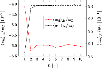
Figure 6. Normalized electrical and mechanical works  and
and  versus number of load cycles
  for the first ten cycles.
Download figure:
Standard image High-resolution image3.1.3. Figures of merit.
In order to evaluate the COR, the quality-assessing quantities according to equation (50) are calculated from the second load cycle and listed in table 1. The negative work output  as well as positive efficiency η basically indicate the cycle's functionality. In conjunction with the negative irreversible electrical work
  , the COR proves to be appropriate, meeting the fundamental idea of a ferroelectric energy harvester. Nevertheless, the total and the ferroelectric efficiencies η and
  are comparably low with values below 10%. In addition, the degree of irreversibility
  of approximately 33% illustrates that while only around one third of the total electrical work
  is harvested from the ferroelectric effect, the remaining two thirds result from the piezoelectric effect. This implies that either the material's properties or the process parameters should be adapted in order to improve the concept's potential.
Table 1. Electromechanical works, degree of irreversibility as well as total and ferroelectric efficiencies in respect of the second load cycle of the COR.
| Quantity | Value | Unit |
|---|---|---|

| −6.2304 | [ ] ] |

| −1.9400 | |

| 93.826 | |
| η | 6.6404 | [%] |

| 31.138 | |

| 2.1633 |
3.1.4. Deficiencies of the COR and idealized cycle.
In order to gain detailed insight into the de- and repolarization processes of the cycle, the courses of normalized macroscopic irreversible polarization  vs the normalized load steps and electric field
  are illustrated in figures 7(a) and (b), respectively. Firstly, in figure 7(a) the simulated course of
  (solid red line) is compared to a theoretical idealized cycle (dashed green line), where de- and repolarization are perfectly balanced. In the more realistic simulations, i.a. grain-interaction and associated residual stresses will prevent this idealization. States of the idealized cycle differing from the simulated one are marked with primes in dashed circles, while all remaining points are identical. At the end of the prepolarization, point ②, an irreversible polarization of
  is achieved. The simulated plot shows that the reduction of polarization from the beginning ② to the end ③ of the harvesting phase P1 is diminutive. On the contrary, a lot of depolarization occurs when turning off the harvesting field from point ③ to point ④, resulting in a decrease of polarization
  , not being exploited optimally in terms of an electric work output. The vanishing loads in the phase of relaxation P2 lead to a further even useless loss of polarization from ④ to ⑤. In fact, ΔP3 4 = 0 with points ③ and ④ being identical and matching the polarization of point ⑤ would be desirable, so that depolarization caused by tensile stress is entirely exploited while the constant harvesting field is applied, thus generating a maximum output of electric work. This is illustrated by the idealized graph in points and , where
  holds the same value of point ⑤, with no loss of polarization during phase P2.

Figure 7. Normalized macroscopic irreversible polarization  of the simulation (solid red line) and an idealized cycle (dashed green line) versus (a) normalized steps of the first load cycle, (b) normalized electric field
  .
.
Download figure:
Standard image High-resolution imageFurthermore, repolarization driven by compressive stress increases  significantly from ⑥ to ⑦. However, the polarization of the initial state ⑩ is not reached. Moreover, when the material relaxes in phase P4, most of the gained polarization is lost when reaching point ⑨. As a result, the harvesting field turned on from ⑨ to ⑩ repolarizes the material instead of the intended mechanical stress, leading to an increase of polarization
  , thus generating considerable electrical work input. In order to reduce the invested electrical work, ΔP9 10 = 0 as well as points ⑧ and ⑨ being of identical polarization as point ⑩ would be desired in P3 of an ideal cycle, see green dashed line with polarizations = = =⑩.
Figure 7(b) illustrates the improvement of the idealized cycle with respect to the electric energy output in comparison to the simulated COR (red area), amounting to a factor of approximately 10. The green area represents the idealized irreversible electrical work that could be additionally obtained, while the gray area represents supplementary energy that has to be invested. Accordingly, a large amount of extra irreversible electrical work  could be obtained, while only a tiny amount
  would have to be additionally invested in the repolarization. Similarily, in phase P3 with ΔP9 10 = 0 the supplementary electrical work output
  could be several orders of magnitude larger than the invested electrical work
  . A parallel can be drawn to the classical Carnot-cycle with its rectangular shape in a T-s-diagram representing the maximum amount of work obtainable in a temperature range.
After all, there are two major conclusions to be drawn from this analysis. Firstly, the tensile stress in harvesting phase P1 is not large enough in order to sufficiently depolarize the material and thus harvest a large amount of electrical work. Secondly, the decrease of  to values around the remanent polarization
  in points ⑤ and ⑨ due to vanishing electrical and mechanical loads is problematic for the quality of the cycle.
3.1.5. Residual stresses and aspects of endurance.
Aside from the harvesting efficiency of the cycle, the lifespan of the device is another important aspect to investigate. Residual tensile stresses will be crucial in this context, giving rise to micro cracking. In figure 8, macroscopic principal stresses  and
and  as well as the maximum values
  and
and  of residual intergranular stresses are compared to the stipulated mechanical load
  . The macroscopic principal stresses represent the volume averages in the polycrystalline RVE according to
As illustrated, they occur during prepolarization when switching processes are initiated at  . In phases P1 and P2, during which tensile stress is prescribed,
  closely follows
  . When compressive stress is imposed during phases P3 and P4, a smaller amount of residual tensile stress is maintained. Due to the definition of maximum principle stress (
 ),
),  closely follows the compressive load in P3 and P4, while being small in the tensile stage of
  . The maximum residual stresses of all grains
  considerably exceed the values of external stress loads in both tensile and compressive regimes. The maximum tensile stress
  being relevant in terms of damage amounts to
which is approximately 175% of the external load.

Figure 8. Normalized loading stress  , macroscopic principal stresses
  and maximum residual principal stresses
  versus normalized load steps of the first cycle.
Download figure:
Standard image High-resolution image3.2. Investigation of influencing parameters
The ferroelectric parameters  and
and  of a hypothetical material on the basis of BT are varied first, followed by an investigation of process parameters. The COR is applied to this material, which is further on denoted as BT*. Just one of the three parameters is altered while the other two are kept constant. It is important to keep in mind that the process parameters
  and
and  are scaled according to the definitions in equations (54) and (55), thus depending on
  and
and  . Electrical and mechanical loads may thus take unreasonably large magnitudes in some cases. In light of this, the investigation may be regarded as hypothetical for certain upper ranges of the material parameters.
3.2.1. Material parameters.
Figure 9 illustrates the influence of the coercive field  on the quality of the COR. The electromechanical works are normalized with respect to material parameters of the original BT in terms of
  thus not depending on the properties of hypothetical materials. In figure 9(a) it is apparent that an increase of
  leads to a considerable augmentation of the negative electrical work
  as well as the mechanical work
  . In figure 5(b), the quality-assessing quantities, according to equation (50), illustrate that this augmentation benefits the quality of the cycle. The total efficiency η monotonically increases with an increase of
  . Furthermore, the degree of irreversibility
  increases as well, exceeding 50% for
  kV m−1. Consequently, the ferroelectric effect increasingly contributes to the electric energy output. The ferroelectric efficiency
  improves likewise due to a boost of the switching processes. The positive impact on the total efficiency is thus not attributed to the piezoelectric but rather to the ferroelectric effect attaining dominance.

Figure 9. Variation of the coercive field; (a) normalized electrical work  and mechanical work
  , (b) total and ferroelectric efficiencies η and
  as well as degree of irreversibility
  versus
  of BT*.
Download figure:
Standard image High-resolution imageThe variation of the spontaneous polarization  is illustrated in figure 10. With regard to the electromechanical works presented in figure 10(a), an increase of
  again leads to a rise, however, several magnitudes smaller than the one observed with
  . The corresponding quality-assessing quantities are depicted in figure 10(b). The total efficiency decreases with an increase of the spontaneous polarization up to
  C m−2 constituting a minimum of η. The increase of
  with
with  exhibits a similar magnitude as observed with
  . The variation of
  , on the other hand, barely influences the ferroelectric efficiency, which only slightly rises with an increase of
  . After all, an enlargement of the spontaneous polarization has a positive effect in a way that while the efficiencies scarcely increase, the ferroelectric effect competes with the piezoelectric effect with regard to the electric energy output.

Figure 10. Variation of the spontaneous polarization; (a) normalized electrical work  and mechanical work
  , (b) total and ferroelectric efficiency η and
  as well as degree of irreversibility
  versus
  of BT*.
Download figure:
Standard image High-resolution imageThe influence of the spontaneous strain  is demonstrated in figure 11. On the one hand, an increase of
  results in a decrease of both
  and
and  , on the other hand, a decrease of
  leads to a considerable increase of both absolute values. The overall changes of magnitudes are similar to those observed with
  in figure 10(a), however, exhibiting a pronounced non-linear behavior. The resulting total efficiency η depicted in figure 11(b) increases when
  is decreased, taking an approximately constant level if
  is increased, due to
  and
and  cancelling each other out. Similarily, the ferroelectric efficiency rises with a decrease of
  , however reduces down to zero and even below when
  is increased. In connection with this, the degree of irreversibility continuously decreases, finally vanishing at
  . Consequently, for
  the ferroelectric effect does not contribute to the energy output, but rather counteracts on it. To summarize, a reduction of the spontaneous strain improves the quality of the COR.

Figure 11. Variation of the spontaneous strain; (a) normalized electrical work  and mechanical work
  , (b) total and ferroelectric efficiency η and
  as well as degree of irreversibility
  versus
  of BT*.
Download figure:
Standard image High-resolution image3.2.2. Process parameters.
Especially the depolarization process in phase P1, which does not act properly as discussed in section 3.1, but also the repolarization in phase P3 could benefit from better adjustment of electrical loads  and
and  and mechanical loads
  and
and  . In the following investigation, one mechanical degree of freedom is eliminated by equating the maximum tensile stress
  and the maximum compressive stress
  according to
  , where
  represents the amplitude of the alternating mechanical load. The parameter space then consists of a bias field
  and a harvesting field
  , as well as mechanical stress amplitudes
  based on the constraints given by Kang and Huber [19]. The electric fields
  and
and  are varied, while the mechanical amplitude
  is held constant. With regard to best exploitation of the ferroelectric effect, the irreversible electrical work
  will be evaluated with a large negative work
  being considered desirable. Results of the parameter study for
  are illustrated in figure 12.

Figure 12. Negative normalized irreversible electrical work  versus normalized electrical process parameters
  and
and  with constant maximum stresses
  ; definition of
  according to equation (54).
Download figure:
Standard image High-resolution imageStarting with a small stress amplitude of  in figure 12(a), it is apparent that most cycles are not functional. The space of most favorable cycles with a positive electric energy output
  is characterized by small bias and large harvesting fields. With increasing the stress up to
  and
and  in figures 12(b) and (c), respectively, the maximum magnitude of
  that can be achieved approximately triples and quadruples. This corresponds to the idea that de- and repolarization work better with increasing tensile- and compressive stress, respectively. Furthermore, a peak starts to form for larger bias fields around
  –
– . When further increasing the stress to
  in figure 12(d), the maximum energy output is again improved and the values of
  for large bias and harvesting fields of
  and
and  , respectively, exceed those of the previous plots with small bias fields. This implies that if the harvesting phase leads to an augmented loss of polarization, the repolarization phase needs more support in terms of a larger bias field. Finally, when reaching large stresses
  and
and  in figures 12(e) and (f), respectively, the space of most favorable cycles is significantly concentrated around large harvesting fields
  to
to  combined with large bias fields
  to
to  . The electric energy output for the best cycles with a stress
  is about ten times larger compared to the small stress cycles. Altogether, the parameter study illustrates that for increasing stress, the electric energy output increases considerably and a combination of large harvesting and bias fields seems to work best. Nevertheless, the best possible cycle with respect to the irreversible electrical work output
  , cannot be found without making use of optimization algorithms, whereupon all four process parameters
  and
and  are variable within the aforementioned constraints.
3.3. Optimization
In the following, an energy harvesting cycle characterized by the four parameters  and
and  will be denoted as 'four parameter process' (4PP). Adding two degrees of freedom in terms of two additional process parameters turned out to have great potential for improving the harvesting process, in the following referred to as 'six parameter process' (6PP). First of all, a 4PP will be optimized with regard to irreversible electrical work output, followed by the introduction and optimization of a 6PP.
3.3.1. Optimization of the four parameter process (4PP).
The optimization of the 4PP can be categorized as a constrained optimization problem, see equation (51). The irreversible electrical work  represents the fitness or target function, i.e.
  . The input parameters are represented by the process parameters, i.e.
  . Furthermore, considering the aforementioned physical constraints for the electric fields and mechanical stresses, the constraint function is given by
In order to approach a maximum of the target function, the evolutionary algorithm outlined in section 2.6 was used. It was stopped after running 3070 simulations, the target function taking almost stationary values. The parameters corresponding to the best cycle, in the following denoted as 'optimized cycle' (OC), are given by
Considering the results of the parameter study in section 3.2.2, the electric process parameters  and
and  in equation (61) match the space of most favorable cycles for
  . However, while for the OC the maximum tensile stress, being aimed at best depolarization, approaches the boundary value
  , a maximum compressive stress
  , being identified in the midst of the parameter range, seems sufficient to repolarize the material. Another optimiziation that takes into account the mechanical work input introducing the target function
  yields a sufficiently identical set of process parameters as in equation (61). As a consequence, if optimizing for maximal irreversible electric energy output, the efficiency seems to be quasi-optimized as well.
The OC is illustrated in figure 13. Comparing the red areas representing electric energy outputs of the COR in figure 7(b) and the OC in figure 13(b), the OC distinctly exceeds the COR. Consequently, the quality-assessing quantities of the OC outclass those of the COR in all respects, see table 2. While the total electric energy output is more than twelve times larger, both efficiencies η and  are improved by several hundreds of percents. The increase of the degree of irreversibility up to
  in particular demonstrates the cycle's enhanced exploitation of the ferroelectric effect. In order to illustrate the reasons for this vast increase in quality of the OC, the polarization is plotted vs load steps in figure 13(a). First of all, there is a significant reduction of
  from states ② to ③, i.e. the depolarization in the harvesting phase P1 works much better compared to the COR in figure 7(a). Although the switching resistance is larger in the OC due to an augmented harvesting field
  , the increased tensile stress leads to much more switching processes than in the COR. Therefore, the ratio of stress-induced and entire depolarization
  is much larger compared to the COR, where turning off the harvesting field is responsible for most of the depolarization. In addition to that, after repolarization, in phase P4 not much polarization is lost when loads have been switched off. As a result, the ratio
  of the OC is smaller compared to the COR since much less of the polarization that was gained in phase P3 is wasted. Altogether, in the OC the depolarization in the harvesting phase could be significantly improved and less polarization is wasted at repolarization. Nevertheless, decrease and increase of polarization ΔP3 4 and ΔP9 10, respectively, as well as the loss of polarization from points ④ to ⑤ could not be avoided.
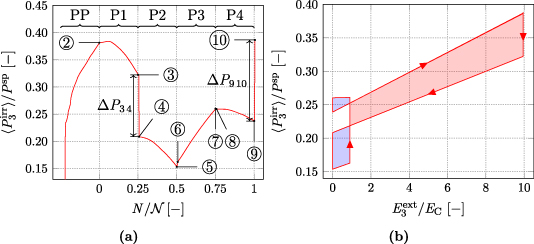
Figure 13. Normalized macroscopic irreversible polarization  of the cycle corresponding to the optimal set of parameters equation (61) versus (a) normalized steps of the first load cycle, (b) normalized electric field.
Download figure:
Standard image High-resolution imageTable 2. Electrical works, degree of irreversibility  as well as total and ferroelectric efficiencies η and
  in respect of the second load cycle.
| Quantity | COR | OC | Unit |
|---|---|---|---|

| −6.2304 | −76.388 | [ ] ] |

| −1.9400 | −37.691 | |
| η | 6.6404 | 29.009 | [%] |

| 31.138 | 49.342 | |

| 2.1633 | 16.780 |
3.3.2. Optimization of the six parameter process (6PP).
The cycles discussed so far are characterized by four independent process parameters  and
and  , constituting four degrees of freedom. In particular, the electric fields of phases of relaxation P2 and P4 are set to zero by default. Consequently, losses of polarization that occur from points ④ to ⑤ and ⑧ to ⑨ do not result in electric work, since there is no electrical resistance against these depolarizations. In order to gain electrical work or reduce the loss of polarization, two extra degrees of freedoms in phases P2 and P4 in terms of electric fields are introduced into a modified harvesting process. It has two mechanical process parameters
  and
and  , as well as four electrical parameters
  and
and  , where each one corresponds to a constant electric field in the respective phase. Consequently, comparing the electric process parameters of the 4PP and 6PP,
  and
and  are identified.
In analogy to the optimization in section 3.3.1, the target function is once again the irreversible electrical work. However, the input parameters are now given by  . The constraints of the electric fields in phases P1 to P4 are those of the harvesting field
  . The resulting constraint function reads
After running 4204 simulations guided by the evoluationary algorithm, the '6PP optimized cycle' (6OC) could be identified and the process parameters are listed in table 3. The electric loading scheme of the 6OC is illustrated in figure 14. In contrast to the previously analyzed 4PP cycles, the electric fields in phases P2 and P4 are now nonzero. While electric fields in phases P2 and P3 are very small according to table 3,  is approximately as large as the former harvesting field
  in phase P1. The application of the 6OC loading scheme leads to results illustrated in figure 15. Comparing the energies in the OC and the 6OC in figures 13(b) and 15(b), respectively, it is obvious that the red area, representing electric energy output, is much larger for the 6OC. In addition, while there is a significant amount of electric energy input represented by the blue area in the OC, there is almost none in the 6OC. The reason for this is the several magnitudes smaller electric field
  of the 6OC compared to the bias field
  of the OC. In order to compare both cycles with regard to their quality in more detail, electromechanical works and quality-assessing quantities according to equation (50) are illustrated in table 4. While the total electric energy output of the 6OC is around two times larger than of the OC, the ratio of the irreversible electrical works amounts to even approximately 2.5. Additionally, the degree of irreversiblity
  now distinctly exceeds 50%, which means that the ferroelectric effect is essentially responsible for the electric energy output. Finally, both efficiencies η and
  are increased by more than 10%. The course of polarization in figure 15(a) illustrates the reasons for the overall improvement. Whereas there is a loss of polarization at the end of phase P2 in the OC, see figure 13(a), the polarization at this point has even increased in the 6OC. The electric field
  at point ⑤ apparently leads to repolarization when tensile stress is decreased, similar to the bias field during phase P3. Moreover, in contrast to the OC, little polarization is lost from points ⑧ to ⑨, due to the large electric field
  even contributing to the electric energy output, whereas in the OC no additional energy is generated in phase P4.

Figure 14. Normalized electric field  versus normalized load steps
  of the first cycle of the 6OC with an excerpt in (b).
Download figure:
Standard image High-resolution image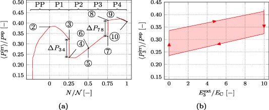
Figure 15. Normalized macroscopic irreversible polarization  of the 6OC versus (a) normalized load steps of the first cycle, (b) normalized electric field.
Download figure:
Standard image High-resolution imageTable 3. Process parameters of the 6OC.
| Process parameter | Value | Unit |
|---|---|---|

| 9.9926 | [ ] ] |

| 2.2645 × 10⁻³ | |

| 8.0797 × 10⁻³ | |

| 9.9729 | |

| 9.9997 | [ ] ] |

| −9.9653 |
Table 4. Electrical works, degree of irreversibility  as well as total and ferroelectric efficiencies η and
  in respect of the second load cycle; 'OC' refers to the optimized 4PP, '6OC' to the optimized 6PP.
| Quantity | OC | 6OC | Unit |
|---|---|---|---|

| −76.388 | −155.89 | [ ] ] |

| −37.691 | −94.398 | |
| η | 29.009 | 41.037 | [%] |

| 49.342 | 60.555 | |

| 16.780 | 29.649 |
After all, the cyclic process in figure 15 meets essential features of the idealized cycle depicted in figure 7, suffering just from naturally given drawbacks of ferroelectric material behavior.
4. Conclusions
Investigating the cycle of reference, weak points in terms of process parameters could be revealed, being responsible for moderate figures of merit. Following the idea of a Carnot process in thermal power machines, an idealized cycle of ferroelectric energy harvesting is identified, optimally exploiting the potentials of re- and depolarization. In a real harvesting process, issues like residual stresses due to domain switching will effectively reduce the idealized efficiency as stress relief inevitably goes hand in hand with a waste of previously gained polarization. A model-based optimization, however, provides process parameters yielding best figures of merit under largely realistic conditions, and suggests a modification of the basic concept introducing two more process steps, finally generating even better harvesting efficiencies. Numerical studies further demonstrate the impact of various material parameters, supporting an appropriate choice of ferroelectric material for harvesting applications. After all, exploiting the ferroelectric and elastic effects in a piezoelectric energy harvester may considerably improve figures of merit. The price to pay will probably be a reduced durability of the device, which has been indicated in the simulations considering induced residual stress.
Footnotes
- 1
The range of remanent polarization experimentally measured for barium titanate is approximately given by
![$P^{\mathrm{r}}/P^{\mathrm{sp}}\in[0.192, 0.308]$](data:image/png;base64,iVBORw0KGgoAAAANSUhEUgAAAAEAAAABCAQAAAC1HAwCAAAAC0lEQVR42mNkYAAAAAYAAjCB0C8AAAAASUVORK5CYII=) [31].
[31].
![$P^{\mathrm{r}}/P^{\mathrm{sp}}\in[0.192, 0.308]$](https://content.cld.iop.org/journals/0964-1726/30/3/035031/revision3/smsabe2bcieqn101.gif)