


Abstract
We present a mathematical model for the protrusion of lamellipodia in motile cells. The model lamellipodium consists of a viscoelastic actin gel in the bulk and a dynamic boundary layer of newly polymerized filaments at the leading edge called the semiflexible region (SR). The density of filaments in the SR can increase due to nucleation of new filaments and decrease due to capping and severing of existing filaments. Following on from previous publications, we present important approximations that make the model feasible and accessible to fast computational analysis. It reveals that there are three qualitatively different parameter regimes: a stable, stationarily protruding lamellipodium; a stable lamellipodium showing oscillatory motion of the leading edge; and zero filament density and no stable lamellipodium. Hence, the model defines criteria for the existence of lamellipodia and the ability of cells to move effectively, and we discuss which parameter changes can induce transitions between the different states. Furthermore, stable lamellipodia have to be able to exert and withstand substantial forces. We can fit the experimentally measured dynamic force–velocity relation that describes how cells can adapt to increasing external forces when encountering an obstacle in their environment during motion. Moreover, we predict a different stationary force–velocity relation that should apply if cells experience a constant force, e.g. exerted by the surrounding tissue.
Export citation and abstract BibTeX RIS

Content from this work may be used under the terms of the Creative Commons Attribution-NonCommercial-ShareAlike 3.0 licence. Any further distribution of this work must maintain attribution to the author(s) and the title of the work, journal citation and DOI.
1. Introduction
Cell motility plays a key role in neural development, wound healing, the immune response [1] and in metastasis of cancer cells [2]. Understanding the mechanisms of cell motility is a prerequisite for finding a means of inhibiting cancer spread [3, 4].
Many motile cells form a lamellipodium in the direction of motion, which is a flat protrusion supported by an actin filament network. The force of protrusion in the lamellipodium is believed to arise from the polymerization of actin [5, 6]. Actin polymers are found in bundles in the interior of the lamellipodium, where myosin motor molecules can move along them to create contractions. Toward the leading edge, actin forms a polar network with the fast polymerizing barbed ends directed toward the membrane. At the opposite pointed ends, filaments depolymerize, actin monomers are recycled and diffuse to the front, where they are consumed by the growing tips [7]. This process is called treadmilling and is regulated by several proteins [8–13]. Arp2/3 (actin-related protein 2/3) binds to an existing actin filament and nucleates a new branch. Arp2/3 is activated by nucleation promoting factors, such as the membrane-associated WASP, N-WASP or WAVE. Activation is restricted usually to the leading edge membrane. Capping proteins bind to the barbed end of a filament and prevent polymerization and depolymerization there. Cofilin binds to filaments, enhances depolymerization and severs them. Different kinds of cross-linking proteins connect filaments and provide mechanical stability to the network. Other proteins are believed to bind actin polymers to the membrane [14].
The protrusions of motile cells consist of the posterior lamellum with highly cross-linked and bundled actin filaments and the anterior lamellipodium with a network of individual filaments polymerizing against the leading edge membrane [15–20]. While earlier studies suggested the lamellipodial actin network to be highly cross-linked very close to the leading edge membrane already due to branching of filaments by the Arp2/3 complex [21, 22], more recent studies showed that the branch point density in the lamellipodium may be rather low and the lamellipodium-like structures may extend several hundreds of nanometers into the cell [23–26]. That view is also supported by the mechanical properties of the anterior region, which is as soft as weakly cross-linked actin networks [6, 27–30]. The studies also differ in their results on filament length. While some conclude that filaments in the lamellipodium have a length of a few hundreds of nanometers [21, 22], others find the length in the micrometer range [19, 23, 24, 28, 31, 32].
The force balance at the surface of the object propelled by actin polymerization comprises forces driving and resisting the motion. Polymerizing actin filaments generate motion [11, 33]. The forces resisting it are only in part drag forces. They arise not so much from the fluid surrounding drops or beads as from friction with the actin network. Cell motion involves membrane motion relative to the substrate and to adhesion sites as well as fluid transport. That also causes forces resisting motion which increase with the velocity. A major contribution to the resisting forces comes from filaments bound to the object surface and pulling on it. That has been shown for beads [5] and oil drops [34] directly. The presence of a large variety of actin binding membrane proteins or proteins linking F-actin to membrane proteins in the leading edge of lamellipodia (reviewed in [14]) strongly suggests that filaments attach also to the membrane and hold it back. Additionally, membrane tension resists protrusion in spreading and motile cells [35–38].
Here, we first present an extension of a model used in a variety of previous modeling studies and then apply the model to questions relevant for cell function. We extend the model to include total filament number dynamics due to capping, nucleation and severing. Changes in filament number were not important for the quantitative modeling of the dynamic force–velocity experiments lasting about 10 s only [30] or morphodynamics on the time scale of a few tens of seconds [39]. But they are so for the stationary response of cells to forces, since the filament number can adjust if force is applied for a long time [40].
The model without capping and nucleation describes the free filament length changes in the semiflexible region (SR). Because shortening of the free filament length by cross-linking is compensated for by filament elongation due to polymerization, all filaments quickly assume the same free length [41]. Based on a monodisperse approximation, we solve equations for the mean filament length. That monodisperse approximation cannot be applied to capped filaments, since they do not polymerize and their length depends on the time of capping. An exact approach requires the time-dependent solution of the partial differential equation for the length distribution dynamics of capped filaments [42]. That can be done analytically but only up to a remaining time integral, which renders the model very slow in simulations and rather inaccessible to analysis. Here, we present the methods and approximations leading in the end to a much simpler model formulation.
We apply the model to calculate the stationary force–velocity relation, but also show that it reproduces the dynamic one. The model enables us also to investigate conditions for protrusion existence. Both, the existence of stable protrusions and the stationary force–velocity relation are crucial for cell behavior in tissue. The existence of protrusions is a prerequisite for mesenchymal (lamellipodial) motion. Since the forces exerted by surrounding tissue on a cell act over a long time, the stationary force–velocity relation applies and not so much the dynamic one which has been measured in vitro [6, 29, 30].
2. The model
2.1. Modeling concept
The model includes the dense cross-linked actin gel in the bulk and the SR at the leading edge of the lamellipodium (see figure 1). The boundary between the gel and the SR is defined by a critical concentration of cross-linkers bound to the actin filaments. The density of filaments in the SR changes by nucleation of new filaments and capping and severing of existing filaments. Filaments in the SR can attach to the leading edge membrane via linker proteins. Attached filaments can not only push, but also pull the membrane. The leading edge dynamics is determined by the balance of filament forces and forces resisting motion.

Figure 1. Schematic representation of the processes included in the model. The actin filaments (green) in the semiflexible region (SR) can fluctuate and bend. They exert forces on the leading edge membrane (blue line) and push it forward. They elongate by polymerization and shorten by attachment of cross-linkers (red dumbbells), which advances the gel boundary (red line) defined by a critical concentration of bound cross-linkers. Retrograde flow in the actin gel counteracts forward motion of the gel boundary. Filaments can also attach to the leading edge membrane and exert a pulling force. New filaments are nucleated from attached filaments. Filaments can get capped or severed and vanish into the gel afterwards.
Download figure:
Standard image2.2. Filament forces
Semiflexible actin filaments are subject to Brownian motion at the length scale of cells since their persistence length lp is in the same range. Filaments of contour length l grafted at one end exert an entropic force on an obstacle at distance z. The force has been calculated in [43] as

with the scaling variable

and

is the critical force for the Euler buckling instability. In [43], it is shown that for small compression  , the scaling function of the entropic force can well be approximated as
For  the calculation yields

The situation is different for attached filaments, since the tip of the filament is always positioned at the membrane and cannot fluctuate. The proteins linking the filaments to the membrane are assumed to behave like elastic springs. We distinguish three different regimes for the force Fa exerted by the serial arrangement of polymer and linker, depending on the relation between the depth of the semi-flexible region z, the equilibrium end-to-end distance R∥ = l(1 − l/2lp) and the contour length l [44]:
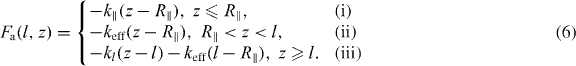
The three cases correspond to: (i) a compressed filament pushes against the membrane; (ii) filament and linker pull the membrane while being stretched together; and (iii) a filament is fully stretched but the linker continues to pull the membrane by being stretched further. Here, k∥, kl and keff are the linear elastic coefficients of polymer, linker and serial polymer–linker arrangement, respectively. For k∥ we use the linear response coefficient of a worm-like chain grafted at both ends k∥ = 6kBTl2p/l4 [45, 46].
2.3. Rates
Detached filaments attach to the membrane with a constant rate ka. The detachment rate of attached filaments is force dependent since a pulling force facilitates detachment. It can be expressed as

with the force-free detachment rate k0d. The length increment d added by an actin monomer to the filament is 2.7 nm.
Detached filaments can polymerize and grow. The velocity of polymerization is force dependent because the probability that the filament fluctuates away from the membrane and a gap sufficiently large for insertion of an actin monomer appears decreases with increasing the force [47]. The polymerization velocity reads

vmaxp is the maximum polymerization velocity depending on the actin monomer concentration.
The rate of filament shortening is contour length dependent. The filaments are shortened by the attachment of cross-linker molecules and incorporation of filament length into the actin gel. The cross-linking velocity is length dependent, since the cross-linker binding probability increases with filament length. It is unlikely that very short filaments get cross-linked. Free cross-linker molecules bind to filaments near the leading edge. Retrograde flow of the actin network transports them as bound molecules to the rear, where they dissociate and diffuse back to the front. Solving the corresponding reaction–diffusion equation, we have shown [48] that the cross-linking velocity can be expressed as

It is proportional to the filament density n, because denser filament packing allows cross-linkers to span the inter-filament distance more easily. The characteristic length  and the maximum cross-linking rate
  are parameters. In the rate of filament shortening
  , the additional factor l/z accounts for the fact that a larger portion of filament length is incorporated into the gel during cross-linking when filaments are bent.
Detached filaments may get capped. The binding rate of capping proteins is force dependent, similar to the attachment of actin monomers to the filament barbed ends during polymerization. We find an Arrhenius factor in the capping rate

New filament branches are nucleated by Arp2/3 off attached filaments with a nucleation rate kn. We assume nucleation from attached filaments since activation of the Arp2/3 complex by nucleation-promoting factors involves membrane binding. New filaments enter the force balance and thus the SR dynamics when they reach the support by the actin gel. Since the branching point vanishes into the gel quickly, newly nucleated filaments have the same length as the mother filament in our model. The total number n of filaments is undefined without a feedback to the nucleation process [42]. Such a feedback could be caused by a limited number of Arp2/3 proteins. The effective nucleation rate reads

The rates k0n and kNn are constants.
We also want to include the disassembly of actin filaments by ADF/cofilin into our model. ADF/cofilin binds to ADP-actin within filaments and promotes its dissociation by severing and depolymerization of filaments [33]. We hypothesize that filaments to which cofilin is bound vanish from the SR because they cannot exert a force any longer once they are severed. Actin filaments bind ATP-actin monomers at their plus ends and quickly hydrolyze ATP to ADP-Pi but it takes longer to lose the y-phosphate. Cofilin only binds to ADP-actin when y-phosphate has dissociated [49, 50]. We can describe the dissociation by an exponential decay. The half lifetime for y-phosphate dissociation within the filament is 6 min [33]. We neglect that y-phosphate dissociation is probably accelerated by cofilin. The probability of cofilin binding is proportional to the probability of finding an ADP-actin monomer at a given site x from the tip of the filament:

We assume that the polymerization velocity is constant vmaxp. The probability of filament severing is found by integrating over the whole filament length

That leads to l-dependent terms in the dynamics of the number of attached and detached filaments.
2.4. Gel velocity and retrograde flow
We have calculated the retrograde flow velocity in the actin gel [48] using the theory of the active polar gel by Kruse et al [51, 52]. It depends linearly on the force acting on the leading edge membrane. Solving the gel equations leads to the expressions for the coefficients of this linear equation as a function of the gel parameters. We obtain for the gel velocity
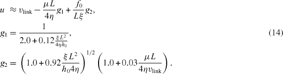
Here, vlink is the cross-linking velocity, hence the velocity at which the actin gel is produced. The gel boundary does not move forward with the velocity of cross-linking since there is a backwards-directed retrograde flow in the actin gel. The term proportional to g1 expresses the retrograde flow arising from contractile stress μ in the actin gel. Contractions may be caused by myosin motors or actin depolymerization [53]. L = 10 μm is the width of the gel part of the lamellipodium and η is the viscosity of the actin gel. The g2-term describes a retrograde flow due to filaments in the SR pushing the gel backwards. The total force that they exert on the gel boundary is denoted by f0. Adhesions between the gel and the substrate are described by the friction coefficient ξ. h0 is the height of the lamellipodium at the boundary between the gel and the SR. We have fit g1, g2 for 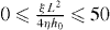 . Equations (14) are valid on the condition that
  .
.
2.5. Dynamic equations
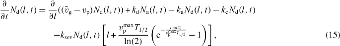
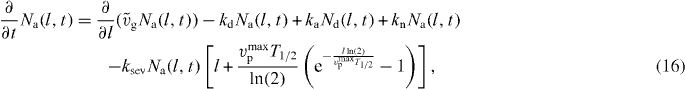
The processes considered so far determine the length distribution of attached Na(l,t), detached Nd(l,t) and capped filaments Nc(l,t) in the SR. Their dynamics are described by the following linear equations (see also [42]):

ksev is the binding rate of cofilin.
As shown in [41, 42], a δ-function-ansatz for Nd(l) and Na(l) used in equations (15) and (16) leads to ordinary differential equations for the total density of attached and detached filaments na and nd and for their mean lengths la and ld:


The dynamics of the SR width reads

with the total filament force

We have also included a constant external force fext that acts on the leading edge. Expression (14) is used for the gel boundary velocity u. The total force of capped filaments fc, the average cross-linking rate vlink and the total filament density n will be calculated below.
2.6. Length distribution of capped filaments
The monodisperse approximation is not valid for the distribution of capped filaments Nc(l,t). That renders the calculation of Nc(l,t) much more complicated than it was for the other densities. However, we need Nc(l,t) for its contributions fc to the force, nc to the total number of filaments and vcg to the average cross-linking velocity vlink (see equation (42)).
Equation (17) is solved using the method of characteristics. Here, we assume that filaments are long when they get capped. We neglect the length dependence of vg and only account for  . As before, we write
  . Furthermore, we are only interested in Nc(l,t) for z ⩽ l ⩽ ld, since for l < z, capped filaments exert no force. Hence,
  . Using the monodisperse approximation for the detached filaments Nd(l,t) = nd(t)δ(l − ld(t)), equation (17) reads

With

we can identify the characteristics

and

The first equation (the first of equations (26)) gives s = t and therefore we obtain

with the solution (obtained by separation of variables)

The time point of capping is denoted by t*. Solving

requires a little more effort. The general solution of the inhomogeneous equation equals the sum of the solution of the homogeneous equation and a special solution of the inhomogeneous equation. The solution of the homogeneous equation reads

The special solution of the inhomogeneous equation is found by the variation of constants:
In the last line, we have used  , where xi are the roots of g(x). Note that l(t*) = ld(t*) at the time of capping t*. Equation (29) yields

We find that
using (29). Furthermore,

Hence,

for  . To find the length distribution of capped filaments, for every length l, t* has to be calculated by solving l = ld(t*). The number of capped polymers is determined by the number of detached polymers and the capping rate at the time of capping.
2.7. The total number, force and cross-linking rate of capped filaments
For calculating the total number, force and cross-linking rate, we need
The total density of capped filaments with z ⩽ l ⩽ ld is then given by

The lower integral boundary is z(t) since shorter filaments do not exert any force and are therefore not considered in the model. The time of capping of filaments with length z at time t corresponds to t*z. We again use equation (29)

and apply a root finding algorithm to determine t*z. The total number of all filaments is given by n = nc + na + nd.
Along these lines, we can also calculate the total force of capped filaments

Note that we have to calculate l(t*) according to expression (29) for every t*. The average cross-linking rate yields

The total number of filaments (attached, detached and capped) n enters vmaxg, and nc is therefore already required for determining t*z (equation (35)). The total number changes according to

It increases by nucleation and decreases because capped filaments are eaten by the gel. We only consider capped filaments longer than z that exert a force in order to simplify the calculations. Capped filaments with length l = z vanish at the rate of gel cross-linking from this filament population. Their number is determined by equation (33) for l(t) = z(t).
2.8. Further approximations
To calculate t*z in every time step and integrate over Fd and vg is computationally very demanding. We also want to avoid tracking the history of la, ld, z, na, nd and n. To simplify the calculation, we assume a stationary distribution Nc(l). In the stationary case, we obtain
We have changed the integration variable according to equation (28).
The total density of capped filaments that exert a force (i.e. with length z < l < ld) reads

With  , we obtain

To calculate the average cross-linking rate,

we again consider only capped filaments with z ⩽ l ⩽ ld. We neglect the length dependence of vg and set vg = vmaxg to obtain analytic expressions

The force of capped filaments is given by

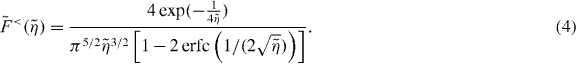
with  (see equation (1)). The scaling function
  (equations (4) and (5)) cannot be integrated analytically. It increases monotonically to 1 with increasing the compression
  of the filament. When simulating the dynamical system we see that the 1/l3-dependence of the integrand of fc dominates over the increasing part of
  (see figure 2). Therefore, we approximate Fd by the Euler buckling force Fcrit and obtain


Figure 2. The force of capped filaments for z ⩽ l ⩽ ld, which occurs in the integrand of equation (44), during a simulation of the system (ksev = 0). (Crosses) The entropic force according to equation (1). (Solid line) Euler buckling force only (equation (3)) with the scaling function set to 1 as an approximation for the entropic force to obtain an analytic expression for the total force of capped filaments fc (equation (45)). Only for lengths slightly larger than z the full entropic force differs from the Euler buckling force, so that the approximated fc is slightly too large. However, the contribution of that part to the integral is very small and the approximation is good. (A) lp = 15 μm and (B) lp = 2 μm. Other parameters: ka = 0.833 s−1, k0d = 1.67 s−1, k0n = 2.0 s−1, kNn = 0.00167 μm s−1, kc = 1.0 s−1,  , vmaxp = 50 μm min−1, κ = 0.833 nN s μm−2,
  , η = 33.3 nN s μm−2, ξ = 10.0 nN s μm−3, μ = 2.78 pN s μm−2, h0 = 0.1 μm, L = 10 μm.
Download figure:
Standard imageIn figure 3, we compare the solution of our time-dependent model with the solution of the model with the approximations introduced in this section.

Figure 3. Comparison of the solution of the time-dependent model (solid lines) and the model with the approximations introduced in this section (dashed lines). (A)–(C) For the parameters from the fit of the force–velocity relation (table 1). (D), (E) For parameters in the regime with n = 0 as the stationary state: k0n = 2.0 s−1, kmaxc = 1.175 s−1, all other parameters remain unchanged. Retrograde flow is set to zero. (A), (D) Density of attached filaments na (blue), detached filaments nd (red) and the total filament density n (black). (B), (E) Force density of attached filaments fa (blue), of detached filaments fd (red) and capped filaments fc (yellow). (C) Length of attached filaments la (blue), of detached filaments ld (red) and SR depth z (black). Filament length is undetermined and increases steadily in the regime with n = 0.
Download figure:
Standard image3. Results
3.1. Existence of stable protrusions
Our model defines criteria for the existence of stable lamellipodia. In figure 4, we examine how the stationary filament density changes with some model parameters. The black areas indicate regions in the parameter space where n = 0 (no filaments in the SR) is the only stable fixed point. Since n = 0 means that there is no protrusion, the conditions for the existence of attractors with n > 0 (fixed points or limit cycles) describe the conditions for the existence of stable protrusions. Different sets of parameters in our model correspond to different cell types or different levels of expression or activation of signaling molecules within one cell type.

Figure 4. Stationary total filament density: (A) as a function of the cross-linking rate  and the nucleation rate k0n; (B) as a function of the capping rate kmaxc and the external force fext; (C) as a function of the binding rate of cofilin ksev and attachment rate ka. There is a bistable domain at large attachment rates. We only show the fixed point with higher filament density. All other parameters are as in table 1.
Download figure:
Standard imageNo stable lamellipodium exists for low nucleation rates in figure 4(A), because the creation of new filaments by nucleation cannot compensate for filament extinction by capping and severing. The stable protrusion vanishes for small cross-linking rates  since the filaments are long. That entails large severing rates and renders the filaments floppy, which increases the capping rate. Similarly, the filament density decreases with increasing capping rate kmaxc (figure 4(B)). A larger external force has among others the consequence of decreasing the capping rate via its force dependence (equation (10)). Furthermore, filaments shorten to adapt to the external force, which decreases the severing rate. In this way, applying an external force may cause protrusion formation in the parameter regime shown in figure 4(B). Nucleation is proportional to the number of attached filaments. Consequently, filament binding may cause protrusion generation in figure 4(C).
Besides stable fixed points with a certain filament density, our model also exhibits stable limit cycles. Those limit cycles also correspond to stable lamellipodia. However, the leading edge shows oscillatory motion and varying protrusion velocities. In figure 5, we show two examples of oscillatory solutions of the model. As already discussed in [41], the membrane velocity can either stay at an intermediate value most of the time and periodically drop to lower values during short 'stops' (figure 5(F)), or the membrane periodically jerks forward during short 'jumps' (figure 5(E)). During the phase of slow movement, attached filaments are shorter than z and pull the membrane. The effective cross-linking velocity  is larger than the effective polymerization velocity vp. Consequently, filaments shorten until the force is sufficiently large to disrupt the attached filaments from the membrane and to push it forward. Now the filaments can grow longer again, exert weaker forces and attach to the membrane (see [41] for a detailed description of the oscillation mechanism). The retrograde flow increases or decreases with the membrane velocity since both are proportional to the total filament force. New filaments are nucleated from attached filaments in our model. Due to the nucleation, the total filament density increases when forces are low and the number of attached filaments goes up (figures 5(A) and (B)). The number of capped filaments also increases, because the capping rate is high at low forces, and the filaments are long and it takes longer until they vanish into the gel.

Figure 5. Examples of oscillatory solutions of the model. (A), (B) The density of attached (blue), detached (red) and capped (yellow) filaments and the total filament density (black). (C), (D) The length of the attached (blue) and detached (red) filaments and SR depth (black). (E), (F) Membrane velocity (black), retrograde flow velocity (red) and the velocity of the gel boundary (light blue). (A), (C), (E) For ka = 0.2 s−1, k0d = 0.5 s−1, kmaxc = 0.23 s−1, vmaxp = 78 μm min−1. (B), (D), (F) For ka = 0.2 s−1, k0d = 0.3 s−1, kmaxc = 0.025 s−1, vmaxp = 12 μm min−1. All other parameters are as in table 1.
Download figure:
Standard imageMany mathematical models equate the leading edge velocity with the polymerization rate or a monotonically increasing algebraic function of it. That excludes a phase difference between the maxima of the polymerization rate and leading edge velocity in oscillations. However, such a phase difference has been observed [54]. The leading edge velocity increases first and subsequently the polymerization rate increases. Figure 6 shows the two oscillation types as limit cycles in the phase plane spanned by polymerization velocity vp and leading edge velocity. The system cycles clockwise in both the cases. The red limit cycle corresponds to oscillations shown in figures 5(A), (C) and (E), and the blue one to figures 5(B), (D) and (F)). The phase difference between both velocities in the red limit cycle is obvious. It is about 9 s expressed in time. That is less than the 20 s observed in [54], but we did not search for parameters with longer delays since the important message is the existence of a clear phase difference. The blue limit cycle exhibits almost no phase difference between the two maxima, but the leading edge velocity decreases earlier than the polymerization rate.
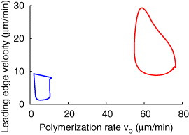
Figure 6. The two oscillation types as limit cycles in the phase plane spanned by polymerization velocity vp and leading edge velocity. The system cycles clockwise in both the cases. The red limit cycle corresponds to oscillations shown in figures 5(A), (C) and (E), and the blue one to figures 5(B), (D) and (F).
Download figure:
Standard imageIn figure 7, we show two examples of bifurcation diagrams where increasing the nucleation rate (figures 7(A), (C) and (E)) or external force (figures 7(B), (D) and (F) leads to a transition from no lamellipodium to a stable, stationarily protruding lamellipodium (a stable fixed point, solid line) to a stable, oscillating lamellipodium (an unstable fixed point, dashed line, a stable limit cycle). In figures 7(A), (C) and (E), the fixed points of the dynamical system are plotted against the nucleation rate k0n. At k0n = 0.25 s−1, the nucleation rate becomes large enough to generate a stable fixed point. Attached and detached filaments are both longer than the SR depth z here. The filament density, and therefore also the cross-linking rate, increases with increasing the nucleation rate k0n. Consequently, filaments get shorter and exert higher forces. Eventually, attached filaments are shorter than z and the effective cross-linking rate may get larger than the effective polymerization rate, leading to a transition to the oscillatory regime. A stable fixed point different from n = 0 can also be generated by increasing the external force (figures 7(B), (D) and (F)). Again, to balance the increasing external force, filaments shorten and their number increases until the fixed point loses stability. Since now the filament density decreases again and the filaments are very short, in the range of the saturation length of the cross-linking velocity, the cross-linking velocity drops below the polymerization velocity and the fixed point becomes stable again upon further growth of force. Note that in those examples attachment rates ka and detachment rates k0d are lower than in figure 4, which is necessary for observing the oscillations.

Figure 7. Stationary filament length, SR depth, filament density, membrane and retrograde flow velocity as a function of the nucleation rate k0n (A, C, E) and the external force fext (B, D, F). (A), (B) The length of attached (blue) and detached (red) filaments and SR depth (black). (C), (D) The density of attached (blue), detached (red) and capped (yellow) filaments and total filament density (black). (E), (F) Membrane (black) and retrograde flow (red) velocity. (Solid lines) A stable fixed point. (Dashed lines) An unstable fixed point; the system oscillates. (A), (C), (E) For ka = 0.2 s−1 and k0d = 0.5 s−1, fext = 0, all other parameters are as in table 1. The displayed fixed points vanish below k0n = 0.25 s−1. However, there is always another stable fixed point with n = 0 and undetermined filament length. Filament lengths larger than 4 μm of the unstable fixed point are not shown in (A). (B), (D), (F)) For ka = 0.2 s−1, k0d = 0.5 s−1, k0n = 0.15 s−1, η = 4.0 nN s μm−2, ξ = 0.7 nN s μm−3, all other parameters are as in table 1. Below fext = 0.008 nN μm−1, n = 0 is the only stable fixed point. Unlike in (A), (C), (E), we only show the stable fixed point that is then generated and not the unstable fixed point.
Download figure:
Standard image3.2. The force–velocity relation
Cells that exhibit stable lamellipodia have to be able to withstand substantial forces from their surroundings. The force–velocity relation describes the lamellipodium protrusion velocity as a function of the force exerted on the leading edge. It is usually measured with a scanning force microscope (SFM) cantilever (see [30]). In [30], we simulated the experimentally measured force–velocity curves with a model with a constant filament density. We now repeat our fit with the model including capping, nucleation and severing. The result is shown in figure 8 and the parameters in table 1. The measured data are still very well reproduced by the model. When the cell touches the cantilever, the velocity of the leading edge drops from ∼250 nm s−1 to less than 1 nm s−1 (figure 8(C)), followed by a concave force–velocity relation (figure 8(B)). As already described in [30], the force–velocity relation mainly gets its characteristic shape due to an initial bending of long filaments and a subsequent adaptation of filament lengths to the increasing external force (figure 8(E)). Retrograde flow slowly increases until it compensates for polymerization in the stalled state (figure 8(C)). The total number of filaments first increases during the concave phase because the capping rate decreases with increasing the force, and severing decreases with shrinking the filament length. Later, the filament number decreases again, because the ratio of attached to detached filaments decreases and therefore also the nucleation rate. The value in the stalled state is slightly higher than in the freely running cell.

Figure 8. Fit of the experimentally measured dynamic force–velocity relation. (A), (B) Comparison of simulation (black) and experiment (red). (A) Time course of the cantilever deflection, which is proportional to the force exerted on the cell. (B) The force–velocity relation obtained from the deflection and the deflection velocity. (C) Development of the leading edge velocity (black), the gel boundary velocity (blue) and retrograde flow velocity (red). The sum of the latter two (dashed magenta) equals the cross-linking rate and is proportional to the filament density. (D) Time course of filament densities: (blue) attached; (red) detached; (yellow) capped; (black) total. (E) Development of filament lengths ((blue) attached; (red) detached) and the SR depth (black). For the parameter values see table 1.
Download figure:
Standard imageTable 1. List of model parameters and their values in figure 8. See also [30].
| Symbol | Meaning | Value | Units | Reference |
|---|---|---|---|---|
| ka | Attachment rate of filaments to the membrane | 10.0 | s−1 | 10 s−1 in [55] |
| k0d | Detachment constant | 25.0 | s−1 | Fitted |
| vmaxp | Saturation value of polymerization velocity | 46.2 | μm min−1 | 30 μm min−1 in [47] |
 |
Saturation value of the gel cross-linking rate | 0.075 | μm2 min−1 | Fitted |
| k0n | Nucleation rate | 0.6 | s−1 | [24] |
| kNn | Limiting factor of the nucleation rate | 0.0016 | μm s−1 | Fitted |
| kmaxc | Capping rate | 0.065 | s−1 | [24] |
| ksev | Binding rate of cofilin | 2.0 | s−1 μm−1 | Assumed |
| T1/2 | Half-life of ATP-actin within filament | 6.0 | min | [33] |
 |
Saturation length of the cross-linking rate | 10 | Assumed | |
| κ | Drag coefficient of the plasma membrane | 0.113 | nN s μm−2 | [56] |
| k | Elastic modulus of SFM cantilever | 291 | nN μm−2 | [30] |
| d | Actin monomer radius | 2.7 | nm | [57] |
| lp | Persistence length of actin | 15 | μm | [58] |
| kl | Spring constant of linker protein | 1 | nN μm−1 | [47, 59] |
| η | Viscosity of actin gel | 0.833 | nN s μm−2 | [60, 61] |
| ξ | Friction coefficient of actin gel to adhesion sites | 0.175 | nN s μm−3 | [62] |
| μ | Active contractile stress in actin gel | 8.33 | pN μm−2 | Fitted |
| h0 | Height of lamellipodium at the leading edge | 0.25 | μm | [63, 64] |
| L | Length of the gel part of lamellipodium | 10 | μm | [21, 64] |
| Contact length with beads | 4.4 | μm | [30] |
Our model fits the measured protrusion and retrograde flow velocities of the freely running cell before cantilever contact, the velocity measured with the cantilever during the concave phase, the value of the stall force and the shape of the force–velocity relation. Due to the good agreement between the measured data and the simulation, we assume that the model parameters determined by the fit of the force–velocity relation represent the 'default' values for the stable keratocyte lamellipodium in parameter space. We can also conclude some features of the structure of the lamellipodium such as filament length and branch point density. The capping, nucleation and severing rates are relatively low. With the filament density of about 280 μm−1 (see figure 8(D)), the effective nucleation rate kn = k0n − kNnn is approximately 9 min−1. Since filaments polymerize in the freely running cell with about 31μm min−1 (the rate of filament elongation equals the rate of filament shortening  ), we should find a branching point approximately every 3.5 μm along the filament. Filaments in the SR are less than 2 μm long and consequently the branch point density is low. If we keep in mind that new branches grow from attached filaments only, we find about 50 branch points in the SR per μm lateral width. The capping rate is also low. The model result for the density of capped filaments in the freely running cell is approximately 10 μm−1 (figure 8(D)). We should bear in mind that this is only the number of capped filaments with lengths between z and ld. Hence, the total number of capped filaments in the SR amounts to 30 μm−1 (see figure 8(E)). Consequently, to accomplish a stationary filament number, the newly nucleated filaments are partly compensated for by capping, partly by severing. In [24], the authors find on average one branch point every 0.8 μm along a filament by evaluating electron microscopy tomograms. However, this value was measured in NIH 3T3 cells and treadmilling is much slower in those cells than in keratocytes, which entails also a smaller branch point distance given a comparable branching rate. The capping and nucleation rates in their simulations (kcap = 0.03 s−1, kbr = 0.042 s−1) are slightly lower but in the same range as in our fit (table 1). Moreover, the actual branch point density should be higher because we only account for filament branches that have already grown to the length of the mother filament in our model.
We would like to emphasize that the force–velocity relation measured with the SFM cantilever is not the relation between a constant external force and stationary velocity values. It gets its characteristic shape due to the adaptation of filament length, SR depth and retrograde flow to the increasing external force. The stationary force–velocity relation with the parameter values from our fit of the keratocyte data is shown in figure 9(A). The stationary force–velocity relation is defined as the stationary protrusion velocity at a given constant external force. It is dominated by the force–velocity relation of the gel (equation (14)) and is almost linear. The slight change in slope occurs because the filament density, and therefore also the maximum cross-linking rate, first increases and then decreases (figure 9(C)). Filaments in the SR shorten to balance the increasing external force (figure 9(E)). However, they remain long enough that the effective cross-linking rate does not drop below its maximum value. Otherwise, we could observe a change in slope (see [48]). We find that the stationary force–velocity relation allows for much faster motion for forces below the stall force than the dynamic force–velocity relation. Cells adapt to the constantly applied external force and become faster by that adaptation. It is not possible that a stationary relation exhibits the initial velocity drop seen in the experiment. If we increase the capping and nucleation rates, the maximum in the filament density is more pronounced (figure 9(D)). Consequently, the stationary force–velocity relation has a concave shape (figure 9(B)). The velocity first increases with increasing force, reaches a maximum and then drops. As we see in figures 7(B), (D) and (F), the force–velocity relation can get much more complex for lower attachment and detachment rates. Here, we enter the oscillatory regime by increasing the external force and observe a drop in the stationary velocity.
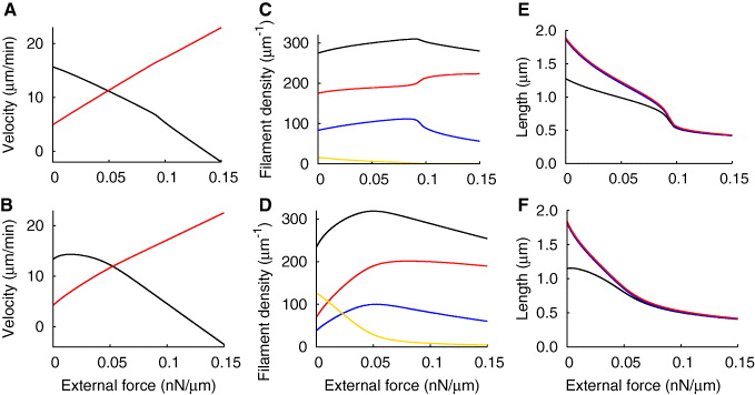
Figure 9. The stationary force–velocity relation and retrograde flow, filament density, filament length and SR depth as a function of the external force. (A), (B) Membrane (black) and retrograde flow (red) velocity. (C), (D) The density of attached (blue), detached (red) and capped (yellow) filaments and total filament density (black). (E), (F) The length of attached (blue) and detached (red) filaments and SR depth (black). (A), (C), (E) For the parameters from the fit of the dynamic force–velocity relation (table 1). (B), (D), (F) For k0n = 2.2 s−1 and kmaxc = 1.0 s−1, all other parameters are unchanged.
Download figure:
Standard image4. Discussion
Our model provides the conditions for the existence of stable membrane protrusions. The existence of critical values for capping and severing above which stable lamellipodia vanish was as expected. Here, we assumed that the binding of the capping protein leads to an elongation of the filament by the diameter of this protein. That renders the capping rate force-dependent. While this paper was in press, we indeed learned about experimental results proving the force dependence of the capping rate, which we had used due to thermodynamic considerations, similar to the force dependence of the polymerization rate [65]. Consequently, large forces may reduce the capping rate to a degree sufficient for protrusion formation. Similarly, filaments have to be short to withstand large external forces, which leads to reduced severing. Since we assumed that membrane-bound filaments do not get capped, and new filaments are nucleated from attached filaments, also membrane binding can rescue lamellipodia. The existence of a critical minimal cross-linking rate illustrates that filaments grow too long and floppy for exerting a force and the lamellipodia collapse, if the gelation process does not keep up with leading edge movement. It is important to keep in mind that transient protrusions may exist with less stringent requirements, such as e.g. a difference between gel boundary and leading edge velocity.
The variation of parameters in this study can be interpreted as describing varying states of signaling pathways converging on lamellipodium formation and control or as describing different cell types. The fit of the measured force–velocity relation determines the parameters applying to the stable keratocyte lamellipodium. We can describe other cell types by varying our model parameters. Thus, our model provides an explanation of why some cells exhibit stable, stationarily protruding lamellipodia while others show oscillations of the leading edge or no lamellipodia at all. Different levels of expression or activation of signaling molecules that entail e.g. different nucleation rates lead to the different phenotypes, while the mechanism for lamellipodial protrusion due to actin polymerization is the same in all cells. Our model also suggests which manipulations should lead to the formation of a stable lamellipodium or vice versa its collapse. For example, reducing the nucleation rate in the keratocyte lamellipodium by inhibiting Arp2/3, or reducing the cross-linking rate by inhibiting cross-linking molecules, should lead to a collapse of the lamellipodium. A transition to a lamellipodium exhibiting oscillating protrusion velocities can be achieved by decreasing the attachment and detachment rates of filaments to the membrane.
The response of the cell to external forces depends on the mode of application. Stationary force–velocity relations are shown in figures 7(F) and 9(A), (B). Application of a constant force leads to a piecewise linear force–velocity relation at small filament nucleation rates and can increase the velocity at larger nucleation rates. Force application may also even shift the cell into an oscillatory regime, as in figure 7(F). These examples illustrate that the stationary force–velocity relation does not exhibit a unique shape but may be rather complex. The comparison between figures 8(B), (C) and 9(A) shows the differences between dynamic and stationary force–velocity relations. Hence, our model predicts that the stationary force–velocity relation is different from the dynamic relations measured by force microscopy in [6, 29, 30]. The differences to the dynamic force–velocity relation arise from adaptation to the force by thinning of the SR and a rise in filament density. That a rise in filament density in response to an increasing external force can entail a constant or even increasing velocity has previously been described in the autocatalytic branching model [40] and has been proposed as the mechanism for the force–velocity relation of actin networks [66].
In a realistic lamellipodium, filaments exhibit a variety of lengths and are oriented under different angles [23, 32]. Length distributions of capped filaments were not calculated explicitly in this study because we were mainly interested in the leading edge dynamics, and short filaments, which cannot exert a force, do not contribute to it. We also do not consider angular distributions. Nevertheless, we are confident that the different regimes found here, no lamellipodia, stable lamellipodia and oscillations, do not depend on this simplification. However, in [67] it was suggested that the filament angular distribution changes under the application of a constant force, and it would be interesting to study whether this influences the stationary force–velocity relation in our model, too. Adhesions are treated as a constant friction between the gel and the substrate in this study. In [30], we have shown that the strengthening of adhesions by the external force does not substantially change the dynamic force–velocity relation. However, further studies are necessary to determine whether remodeling of adhesions contributes to the stationary force–velocity relation.
We have also not included any signaling events in our model. This is certainly a good approximation for the measurement of the dynamic force–velocity relation which takes 5–15 s. Signaling would need to occur even faster. Given, additionally, that the model explains a variety of experimental observations starting with the shape of the complete relation on physical grounds, it seems unlikely that signaling has an essential role in shaping the dynamic force–velocity relation. However, one can imagine that cell signaling, and therefore also our model parameters such as nucleation or polymerization rate, change and adapt if a stationary force is applied to the lamellipodium. Our simulations of the stationary force–velocity relation allow determining whether signaling has a role there by comparing our results with future experiments. Moreover, it is interesting to note that signaling is not necessary for the adaptation of the filament density to the force.