


Abstract
Stable operation of complex flow and transportation networks requires balanced supply and demand. For the operation of electric power grids—due to their increasing fraction of renewable energy sources—a pressing challenge is to fit the fluctuations in decentralized supply to the distributed and temporally varying demands. To achieve this goal, common smart grid concepts suggest to collect consumer demand data, centrally evaluate them given current supply and send price information back to customers for them to decide about usage. Besides restrictions regarding cyber security, privacy protection and large required investments, it remains unclear how such central smart grid options guarantee overall stability. Here we propose a Decentral Smart Grid Control, where the price is directly linked to the local grid frequency at each customer. The grid frequency provides all necessary information about the current power balance such that it is sufficient to match supply and demand without the need for a centralized IT infrastructure. We analyze the performance and the dynamical stability of the power grid with such a control system. Our results suggest that the proposed Decentral Smart Grid Control is feasible independent of effective measurement delays, if frequencies are averaged over sufficiently large time intervals.
Export citation and abstract BibTeX RIS

Content from this work may be used under the terms of the Creative Commons Attribution 3.0 licence. Any further distribution of this work must maintain attribution to the author(s) and the title of the work, journal citation and DOI.
1. Introduction
A major challenge in realizing a future sustainable power supply is the volatile character of many renewable sources [1–3]. The power generation of wind turbines and photovoltaics fluctuates strongly on different time scales: in addition to the obvious variations between the seasons and during a single day [4], strong fluctuations occur on much shorter time scales, for instance due to the turbulent character of wind [5]. To match generation and demand in a fully renewable power grid for the current demand characteristics at every point of time, would thus require large storage facilities. Current estimates for the storage capacity range up to 400 TWh for the entire European grid with 100% renewables and no stand-by power plants [4]. In addition to potential environmental effects, as, e.g., the large landscape consumption for pumped hydro storage facilities, this would require massive capital investments.
To reduce these enormous numbers, it has been proposed to regulate the consumer demand to match the fluctuating power generation [6]. This is a massive paradigm shift in the operation of power grids, as mainly the generation is regulated in current power grids [7, 8]. In the new system, the price of electric energy shall be adapted to the current generation to provide a stimulus for the consumers to adapt their demand. Most proposals for such a smart grid are based on a sophisticated information and communication technology infrastructure. All 'smart' power meters communicate with a central computer in order to negotiate the price and control their demand (see, e.g., [9]). However, such a centralized system would also raise questions of cyber security and privacy protection [10, 11]. Even more, it has been shown that interdependent systems, such as this, can become vulnerable to cascading failures [10, 12].
An alternative, decentralized approach has been first proposed already years ago, but received a major interest only recently. The key idea is that the grid frequency provides all information needed to control the grid. The frequency increases in times of excess generation, while it decreases in times of underproduction [13, 14]. In current power grids, the primary control of conventional power plants is already based on the frequency: generation is increased when the frequency decreases and vice versa [15]. In a future, fully renewable grid the consumers could take over this role and regulate their demand autonomously on the basis of the grid frequency. To make this economically favorable, it was proposed that the price of electric energy for each local consumer is a direct function of the local grid frequency [16]. Is such a decentralized approach capable of ensuring stable network dynamics?
Here we analyze systems with prices locally computed as a direct function of local frequency, taking into account averaging time intervals and effective time delays. We demonstrate that the approach holds risks at certain time delays if the averaging interval is short. Intriguingly, for sufficiently large averaging interval, network dynamics is stable, independent of the delays. Our modeling results thus suggest that Decentral Smart Grid Control provides an efficient measure of ensuring grid stability.
The article is structured as follows. First, we introduce a mathematical model for the frequency dynamics of a power grid, describe our concept of a Decentral Smart Grid Control to realize the dynamic demand response (DR) in section 2 and discuss several economic aspects in section 3. The dynamics and stability of a fully interdependent techno-economical system are then analyzed in detail in section 4. We uncover potential systemic risks and show how they can be mastered by a proper implementation of the control.
2. DR via Decentral Smart Grid Control
DR is generally based on a flexible consumer price for electric power which is adapted to the current power generation. In periods of higher demand than generation, prices are high, giving an incentive to the consumers to reduce their consumption. Current approaches for the implementation of DR are mostly based on centralized information and communication infrastructure [8, 9], i.e., all information about production and consumption is collected decentralized, transmitted to one central IT-unit which then sends commands for further consumption and production to the decentralized actors. Such a system would require large financial investments and raises concerns about data protection and system vulnerability [10–12]. However, such an expensive IT-infrastructure may not be needed, as the grid frequency already encodes the necessary information and is accessible everywhere in the grid.
To analyze the essential frequency dynamics of a large-scale power grid and its coupling to pricing information we consider an oscillator model based on the physics of coupled synchronous generators and synchronous motors, which recently attracted a strong interest in physics [17–23]. This model is very similar to the 'classical model [15] and the structure preserving model [24] from power engineering, which are routinely used to simulate the dynamics of power grids on coarse scales.
The state of each rotatory machine j is characterized by the rotor angle  relative to the grid reference rotating at
  or
or  Hz, respectively, and its angular frequency deviation from the reference
  . Every machine has its moment of inertia Mj and is driven by a mechanical power
  , which is positive for a generator and negative for a consumer. In addition, every machine is driven by the electric power transmitted via the adjacent transmission lines which have a coupling strength Kij. The dynamics of the machine j is then given by the equation of motion as

For a more detailed discussion and short derivation of the equations of motion, see appendix
For the sake of simplicity, we assume that all damping constants  and moments of inertia
  are identical for a while. The overall angular frequency deviation
  is then determined by the equation of motion

where  is the total power balance in the grid. Equation (2) can be solved analytically with the result

For  , the overall angular frequency deviation
  converges to the value
  . This relaxation is typically fast; most perturbations are cleared in less than a second [15]. In weakly connected grids inter-area oscillations can last for a minute [3, 26]. Hence, the angular frequency deviation
  is directly proportional to the power balance of the entire system. In general, the angular frequency is the same throughout the grid
  and can easily be measured, such that it can be used to control the grid without additional communication infrastructure.
The missing step to realize a Decentral Smart Grid Control is to come up with a one-to-one relation between the local grid angular frequency deviation  and the current electricity price
  . A device that measures the local grid angular frequency and calculates the current price according to this pre-defined function
  is cheap and can be implemented in a decentralized way, see [28] for large-scale frequency monitoring. Electric devices with an on-off load characteristic (e.g. washing, refrigeration, thermal heat pumps, electric cars) could automatically shift their consumption to times of high grid frequency, relieving the grid in low frequency times. Ensured by a properly chosen price function
  , this grid service can be economically reasonable for the consumer and also for the electricity provider, because the grid operator would have potentially less costs for primary, secondary and tertiary control. A drastic price increase at low frequencies and cheap electricity at high frequencies might also change the active consumer behavior. The needed technology is readily available, since micro combined heat and power systems or photovoltaic systems, already have a comparable control system included [8, 27].
In particular, we propose a Decentral Smart Grid Control that realizes a dynamic DR in power grids and analyze some of its core economic and dynamic consequences. The mechanical power  in the equation of motion (1) is the difference of the generated and consumed power at the jth node of the network. Both generation and consumption depend on the current energy price p, which is described by supply S(p) and demand curves D(p), such that we find

A supply function S(p) gives the amounts of goods offered, if this good is traded for a certain price p. Here, this is the amount of power supplied by a generator, if the obtained price is p. Similarly, the demand D(p) gives the amount of power a consumer would like to consume for a given price p. Generally, the supply curve is monotonically increasing with p, while the demand curve is monotonically decreasing. The two curves are exogenous to the model, in fact they are determined by the strategy of the generators, the weather and the preferences of the consumers.
We suggest a Decentral Smart Grid Control that calculates the price on the basis of the local angular frequency deviation  [16]; but measuring and updating the angular frequency in a real grid takes a certain time. Therefore, the price generally depends on a time-averaged angular frequency deviation
  . Assuming that the angular velocity is measured over an interval of fixed period length T, we define

We consider two technical scenarios for the control. First, we consider a control system that adapts only in discrete time steps of length T such that the local prices are given by

where  denotes rounding towards minus infinity. Second, it can take a certain delay time τ until the control system adapts such that the local prices are given by

We assume that the price only depends on the frequency and that supply and demand curves are given and keep their form on the time scales (seconds) described in this article. Hence, the design of an appropriate price function  is an important step for the implementation of a DR via Decentral Smart Grid Control.
3. Economic aspects
3.1. Benefits of DR
DR may have huge benefits in future energy systems see, e.g., [7, 8, 25, 29, 30]. Here, we briefly summarize the most important economic aspects, following [7], which hold regardless of the technical implementation: (1) consumers may reduce their electricity bill by shifting their demand to periods of low prices. (2) In addition, DR may reduce the global costs of the power system as it allows for a more efficient use of the existing infrastructure and avoids costs for additional infrastructure. (3) DR may improve system stability by avoiding dangerous peaks of the demand and thus reduce the probability of power outages. (4) Finally, DR may improve market performance and reduce the price volatility. In addition to these points, DR is particularly important for future power grids because its implementation can potentially allow a higher penetration with renewable energies [31].
3.2. The grid as a market
In the current proposal of a Decentral Smart Grid Control there is no central computer which controls the demand of the consumers and no central exchange to determine the electricity price. The control is realized in a decentralized way using local frequency measurements, thus requiring no long-distance communication. Is this sufficient to provide an efficient market, i.e., to reach an economic equilibrium?
To answer this question we first note that the stable stationary operation of a power grid requires that all machines rotate in synchrony, i.e., the frequency must be the same everywhere

Otherwise the power flow between two nodes j and k

would be oscillating and average out over time. The synchronous state must be dynamically stable for small disturbances to be damped out [15, 32] and the grid may self-organize to a synchronous state with steady power flows [18, 22, 33]. Substituting the condition  into the equations of motion (1) shows that the synchronous state is determined by the equation

Summing up the equations for all j and using  yields

This shows that a dynamical equilibrium of the grid also implies the economic equilibrium of the market, i.e., the supply equals the demand including transmission losses. Hence, we have to analyze the dynamic stability of the combined techno-economical system to evaluate its stability properties. This will be done in detail in section 4.
For now, we assume that the grid is in equilibrium with  at a price
  . To analyze the stability of this equilibrium, we linearize the supply and demand curves close to the equilibrium:

The modeling or measurement of supply and demand curves then reduces to the measurement of the elasticity of supply and demand. Generally, the supply increases with the price while the demand decreases such that  and
and  and thus in particular

Here, we used course-graining, i.e., not every consumer is represented by one demand function but several consumers are aggregated to form one node in the network and hence supply and demand curves are assumed to be smooth.
3.3. Price and frequency fluctuations
The new aspect of our proposal of a Decentral Smart Grid Control is the direct encoding of the electricity price in the grid frequency. Thus, the grid frequency must be allowed to vary in certain boundaries so that fluctuations of the price are directly related to fluctuations of the frequency. Currently, frequency variations are limited due to technical reasons [34]. In the European grid  are acceptable in normal operation and up to
  can occur in extreme cases for short times before emergency measures such as load shedding are initiated [35]. This sets the order of magnitude at which the frequency may vary. Accordingly, we consider a frequency range of
  .
.
In figure 1 we analyze the possible variations of the price and the frequency in more detail. Panel (a) shows a histogram of plausible values of the consumer price, if this price is strictly coupled to the variable spot market price for Germany in 2012 [36]. To obtain plausible consumer prices, we add 9 ct kWh−1 for distribution and service, 7 ct kWh−1 fees plus 19% VAT on the total. The variations of the electricity price directly relate to variations of the grid frequency as described above. We consider a linear price curve for all nodes

with  ct kWh−1, as shown in panel (b1). For a slope
  (ct kWh−1)/2π Hz, the price curve maps the operational range
 ![$({{\bar{\omega }}_{j}}+\Omega )/2\pi \in [49.5,50.5]$](https://content.cld.iop.org/journals/1367-2630/17/1/015002/revision1/njp505903ieqn35.gif) Hz to a price interval
Hz to a price interval ![$p\in [19.1,29.1]\;{\rm ct}\;{\rm kW}{{{\rm h}}^{-1}}$](https://content.cld.iop.org/journals/1367-2630/17/1/015002/revision1/njp505903ieqn36.gif) , which covers 98% of the observed fictitious consumer prices. A histogram of the resulting frequency variations is shown in panel (c1). In 2% of all time slots prices outside of this interval were recorded which can even become negative.
, which covers 98% of the observed fictitious consumer prices. A histogram of the resulting frequency variations is shown in panel (c1). In 2% of all time slots prices outside of this interval were recorded which can even become negative.

Figure 1. In DR via Decentral Smart Grid Control, variations of the electricity prices imply variations of the grid frequency. (a) Histogram of plausible fully flexible consumer prices deduced from spot prices at the European energy exchange [36]. (b) Price-frequency relation according to (b1) equation (14), with slope  and (b2) equation (15), with
  and
and  , respectively. (c) Histogram of the corresponding frequency fluctuations.
Download figure:
Standard image High-resolution imageTo treat such events accordingly, a nonlinear function must be chosen which maps a fixed finite frequency interval to all possible prices, i.e., to the real line. Still, the slope of this function should be bounded around the operational point  Hz. These requirements are satisfied by an inverse sigmoidal function. As a particular example, we here consider the function

which maps all angular frequency deviations in the interval  to a price
  . The operational range can thus be fixed beforehand, and emergency measures can be specified, if frequencies outside this range are measured. Choosing
  yields the same slope of the price curve around the reference frequency as the linear price function (14). Indeed, using
  Hz the statistics of the observed frequencies in figure 1 hardly change in comparison to the linear price function, see panels (b2) and (c2). The corresponding frequencies change significantly only for extreme price events, which now map to the operational range
 ![$({{\bar{\omega }}_{j}}+\Omega )/2\pi \in [49.5,50.5]$](https://content.cld.iop.org/journals/1367-2630/17/1/015002/revision1/njp505903ieqn45.gif) Hz as desired. A similar statistic is found for other sigmoidal functions. The precise form of such a nonlinear price function can be designed by the grid operators on the basis of actual market and consumption data.
Hz as desired. A similar statistic is found for other sigmoidal functions. The precise form of such a nonlinear price function can be designed by the grid operators on the basis of actual market and consumption data.
We note that figure 1 is based on the German spot market prices, which show huge fluctuations compared to other energy markets [39]. Furthermore, one major effect of a comprehensive DR would be to suppress extreme price fluctuations anyway [7, 14]. Hence, we expect that the fluctuations shown in the figure represent extremes, and that they would be significantly smaller in energy systems with DR and (virtual) storage.
4. Dynamics and stability
Dynamical stability is a basic requirement for power grid operation [3, 15]. For DR via Decentral Smart Grid Control, a stable dynamic equilibrium ensures that the energy system is also in an economic equilibrium as shown above. However, stability properties may become much more involved due to the interdependency of the technical and the economical subsystem. Interdependencies may introduce new systemic risks to dynamical network systems [12, 37].
The interaction of the DR system with the grid depends crucially on their time scales. In contrast to current energy markets, the price can be adapted in almost real time, limited only by the time needed for a frequency measurement. Here, we analyze the dynamical stability of the full techno-economic system and identify new systemic risks for different scenarios and discuss how to master these risks.
4.1. Instantaneous adaption
We first investigate a DR that is fast compared to the grid dynamics. Assuming an instantaneous adaption of the demand, i.e.,  in equations (6) and (7), the effective power
  in equation (1) becomes a function of the current angular frequency deviation
  . In particular, we consider a linear relation of price and angular frequency deviation

Linearizing the supply and demand curves around  as in equation (12) yields

By equation (13), an instantaneous economic response thus increases the effective damping constant to

Therefore, it always lowers the return times after perturbations, see equation (3).
4.2. Slow adaptation in discrete time steps
A second, more realistic scenario is that the Decentral Smart Grid Control is much slower than the grid dynamics. Here, we consider a discrete time control system, where the price function is the same for all nodes and given by (6). Both supply and demand are updated periodically with periodicity  . Assuming that the grid is dynamically stable for the given parameters, the angular frequency deviation will relax to

On this basis, a new market price  is calculated. Assuming an affine-linear price function as in equation (14) and using the linearized supply and demand curves (12), we find

This yields an oscillating dynamics of the market price, which is stable if and only if

setting a strict upper limit for the slope of the price function. The potential instability for  is caused by an overreaction of the suppliers and consumers to market incentives. Similar rebound effects can generally occur in DR systems [8], such that this problem is not specific to the current proposal.
An example for the possible dynamics of the techno-economical system is shown in figure 2 for a model grid with three generators and three consumers with values inspired by the IEEE 9-bus test grid (see panel (e)). We assume that the price elasticities

are the same for all nodes and given by  and
and  in agreement with empirical results [38–40]. The price and subsequently the demand and supply are adapted after a time step of T = 60 s. We assume an equilibrium price
  ct kWh−1 and a damping constant
  with
with  . All transmission lines have the same transmission capacity K = 200 MW. For these parameters, the system is stable if and only if
  . Otherwise the prices and the grid frequency will diverge after a small perturbation as shown in figure 2.

Figure 2. Dynamics of a model grid with Decentral Smart Grid Control in discrete time steps of T = 60 s. System stability depends crucially on the slope of the price curve, being stable for (a, b)  and unstable for (c, d)
  . We plot the dynamics of (a, c) the local prices pj and (b, d) the local frequencies
  starting from an initial price
  ct kWh−1 above the equilibrium price
  ct KWh−1. The angular frequency deviations
  vary only very little from node to node as shown in the inset in panel. (b) These residual oscillations relax on longer time scales such that the system in (a, b) converges to a fixed point with
  and
and  . The model grid is depicted in panel, (e) where generators colored in red and consumers in blue. The remaining system parameters are given in the main text.
Download figure:
Standard image High-resolution imageWe note that this result can be interpreted as an application of the famous cobweb theorem from microeconomics [41] to Decentral Smart Grid Control. The generalized equilibrium condition (11) can be seen as the intersection of the loss curve  and the net supply curve
  . The loss takes the role of an effective demand function with fast relaxation, while the net supply is adapted much slower. The cobweb model then states that the economic system will relax to an equilibrium, if the slope of the loss curve is larger than the slope of the net supply curve, which yields the stability condition (21).
4.3. Delayed adaptation: risks from resonances
New risks may emerge when the Decentral Smart Grid Control acts on similar time scales as the dynamics of the grid such that the two system become truly interdependent. We first consider the case of a delayed feedback, i.e., we consider the price function (7) with  but without averaging (T = 0), i.e., consumers measure their local frequency and try to adapt as fast as possible but need their intrinsic time τ to react. To obtain analytic solutions for the interdependent techno-economical system, we use a very simple system: we linearize the supply and demand curves (12) and consider only two nodes with equal technical and economical parameters, i.e.,
  ,
,  ,
,  and
and  . Defining our new variables as the phase difference
  and the angular frequency difference of the two nodes
  , the equations of motion read

where we introduced the abbreviations  ,
,  ,
,  ,
,  and
and  . In the following, time is measured in seconds, α and γ in s−1 and P and K in s−2. This notation is similar to the one used in [19]. Delayed differential equations need a history function as initial condition, which we chose to be
  for our dynamical simulations. Furthermore, we used standard mathematica routines [42] to solve the ordinary and delayed differential equations.
The delayed adaption of supply and demand can both stabilize and destabilize the grid dynamics as shown in figure 3. The physical reason of this effect can be easily understood. The frequency-adaptive 'effective' power  in equation (23) can be seen as a resonant driving acting on an oscillating system. Such a driving term will either damp or amplify the oscillations depending on whether the driving is in-phase or out-of-phase. The phase shift of this driving term is directly given by the delay τ, such that the stability of the system depends crucially on the value of τ. To illustrate this result, we compare the dynamics for two different values of τ in figure 3. For
  the driving is in-phase, the oscillations are amplified and the grid becomes unstable with potentially fatal results, whereas
  stabilizes the system.
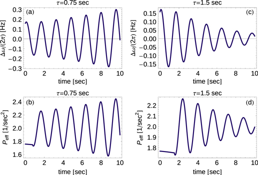
Figure 3. Decentral Smart Grid Control can stabilize or destabilize the grid. Panels (a)–(d) show the frequency difference  and effective power
  for an elementary two-node network as a function of time for two different delays, according to (23). For the delay
  the effective power becomes large simultaneously to the frequency difference, i.e., the generator produces more energy than needed, when the frequency is already too high, see (a) and (b). Hence, the system gets destabilized completely. On the contrary, the effective power and frequency difference are shifted by half a period for
  such that the system is stabilized, see (c) and (d). Initial conditions were
  ,
,  Hz and the parameters
  ,
,  ,
,  ,
,  were applied.
Download figure:
Standard image High-resolution imageTo obtain a global view of the stability and the role of the system parameters we analyze the dynamical stability around the steady-state operation of the grid given by the fixed point

A solution exists only if the transmission capacity is larger than the power which has to be transmitted,  [32]. The linear stability of a dynamical system is determined by the eigenvalues of the Jacobian matrix. For a delayed system [43–45], we have to calculate the Jacobian of both the non-delayed system, based on equation (23),

and the derivatives for the delayed term

where we consider exponential solutions, see [45]. The stability eigenvalues λ are then determined by the solution of the characteristic equation

Small perturbations induce an oscillatory motion with eigenfrequency  and period
  . The amplitude grows or decreases exponentially as
  such that
  is the condition for a dynamic instability. This is possible only if the frequency adaption is strong enough compared to the damping of the system,

as shown below. When the delay τ changes, we observe a periodic pattern of stable and unstable parameter values as shown in figures 4 and 5. As explained above, destabilization occurs in the case of an in-phase driving which happens when τ is an integer multiple of the period of the eigenoscillations of the system.
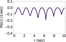
Figure 4. The stability exponent  plotted as a function of the delay τ for an elementary two-node network. The dynamic becomes unstable, i.e.,
  , for certain values of the delay time τ periodically spaced on the real axis, if
  . Parameters are
  ,
,  ,
,  and
and  and the root with highest real part of equation (27) was obtained numerically using Newtonʼs method.
Download figure:
Standard image High-resolution image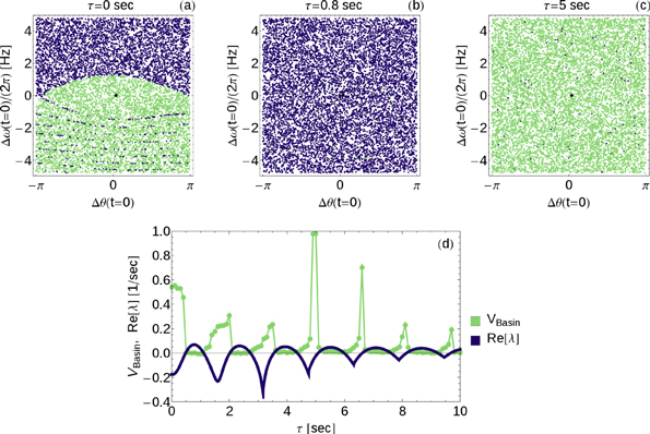
Figure 5. The global stability of a two-node network with Decentral Smart Grid Control is quantified by the volume of the basin of attraction and compared to linear stability. Both measures predict instability for similar delays τ. A visualization of the basin of attraction for different values of the delay τ is shown in panels (a)–(c). Light green dots represent initial conditions that converge to the fixed point while dark blue dots assume a limit cycle or converge too slowly. Parameters are  ,
,  ,
,  ,
,  and 10 000 different initial conditions were used. In panel (d) the basin volume
  (discrete plot, light green) is plotted as a function of τ in comparison to the stability exponent
  (dark blue). We used the same parameters but only 1000 different initial conditions.
Download figure:
Standard image High-resolution imageTo proof these statements we first note that  for
for  or
or  as long as
  . We now consider the parameter values where
  changes its sign such that the system becomes unstable. Decomposing the characteristic equation (27) into real and imaginary parts and setting
  yields the conditions


The second equation can be solved for τ with the result

One directly sees the periodicity in the delay τ, where the period  is equal to the period of the eigenoscillations of the system. Furthermore, the
  is real only if
  , which yields a necessary condition for the destabilization by delay. Note that this statement is equivalent to the one from section 4.2, namely the damping of the system has to be larger than the price influence to always guarantee stability.
In addition to the local stability analysis, we also consider the grid dynamics after a large perturbation. We integrate the equations of motion for a long time period until  with initial conditions randomly drawn from a subset of the phase space
 ![$Q=[-\pi ,\pi ]\times [-30,30]\;{\rm Hz}$](https://content.cld.iop.org/journals/1367-2630/17/1/015002/revision1/njp505903ieqn123.gif) , see also [46], and evaluate whether the system relaxes to a stable operation, i.e., whether it converges to the fixed point (24), or not. As a criterion for stable operation we assume an angular frequency deviation of
, see also [46], and evaluate whether the system relaxes to a stable operation, i.e., whether it converges to the fixed point (24), or not. As a criterion for stable operation we assume an angular frequency deviation of  . The results are visualized in figure 5, panels (a)–(c), where we plot the stability in a color code (light green: stable, dark blue: unstable) as a function of the initial location in phase space for different values of τ. The results confirm the finding of the linear stability analysis. Depending on the value of τ the global stability is altered dramatically. For
  the fixed point is linearly unstable and the system does not relax for almost all initial conditions. On the contrary, a delay of
  leads to an almost perfect stability; the grid converges for almost all initial states. Notably, the regions of initial conditions leading to stable or unstable behavior are not clearly separated because the actual boundary of these regions has a rather complex geometric structure already in the non-delayed case.
The global stability of a fixed point of a dynamical system can be quantified by the volume of its basin of attraction. The 'basin size'  can be determined numerically using a Monte Carlo method as the ratio of initial conditions converging to a stable operation to the total number of initial conditions. Figure 5 panel (d) shows how the basin volume depends on the delay time τ in comparison to the linear stability exponent
  . As expected,
  tends to zero in the case of linear instability,
  . Maxima of
  of different height are observed in the stable parameter regions, including an almost perfect stabilization for
  . However, these maxima do not coincide with the minima of
  As both the linear stability and the basin volume predict similar delays to be problematic for the system, we focus on the computationally easier to handle linear stability in the following.
4.4. Stabilization by averaging
Measuring the local grid frequency will generally take some time in a real-world system. We thus consider the dynamics of the elementary model grid for the price function (7) including both delay  and averaging over a period
  . The equation of motion for the angular frequency difference
  then reads

The integration can be carried out in a straightforward way by using (23) such that we obtain the modified delayed dynamical system

To evaluate the stability of the steady state (24), we have to calculate the eigenvalues λ for a system with both the delay τ and the delay  . The Jacobian of the non-delayed system is given by (25) as above and for the delay terms only
  and
and  are non-zero. The stability eigenvalues λ are then given by the roots of the characteristic equation [43]

Figure 6 shows the real part of the stability eigenvalue  as a function of the delay τ and the averaging time T. Instabilities are observed for certain values of τ, if T is small as discussed above. But for a sufficiently high T, the system stays stable regardless of the time τ. The actual values of the stability exponent
  for large
  are comparable to the one of the system without any price adaptation.
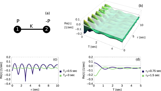
Figure 6. Frequency averaging stabilizes Decentral Smart Grid Control for delayed feedback. Averaging over an interval of sufficient length T guarantees stability for all  . The figure displays a scheme of the system in panel (a) and the stability exponent
  for the system according to characteristic equation (34) as a function of delay τ as well as the averaging length T in panel (b). A transparent layer is added at
  Cuts for two different but fixed averaging times T in panel (c) and for two different but fixed delays τ in panel (d) are added. Parameters are
  ,
,  ,
,  and
and  and Newtonʼs method is used to obtain λ.
Download figure:
Standard image High-resolution imageThe results shown here are very interesting: while a delay in adaptation poses a stabilization risk to the grid, averaging the measured signal for a certain time removes the short time fluctuations that could resonantly drive the system and thereby guarantee a stable operation state. Still, the nodes can adapt to changes of the generation on all time scales slower then T, which provides an effective DR management system.
4.5. The role of the network topology
The larger the grid becomes, the more complex behavior it is able to show. Here, we consider a network with four nodes to test our results. Two consumers ( ) are supplied by two generators (
 ). Each generator is coupled to a consumer to balance the power production/consumption. In addition, the generators are coupled to each other. As above we assume that all technical and economic parameters are the same for all nodes of the network. The equations of motion can be read in appendix
Risks from resonant driving emerge in a grid with delayed response and T = 0 as discussed above. The grid becomes unstable in certain regions of parameter space which are periodically spaced on the τ-axis. In a complex network, there are generally many different eigenmodes with different frequencies. The parameter regions where these modes can be excited generally overlap, such that the grid becomes unstable for most values of the delay τ as shown in the dark blue curves of panels (c), (d) in figure 7. Only for a very fast response  the dynamic is stabilized.

Figure 7. In networks only non-delayed systems, i.e.,  , T = 0 stabilize the system while for a delay
  , an averaging time
  is required. Hence, averaging is even more important to ensure stability for larger systems. The figure displays a scheme of the system in panel (a) and the stability exponent
  for the system as a function of delay τ as well as the averaging length T in panel (b). A transparent layer is added at
  Cuts for two different but fixed averaging times T in panel (c) and for two different but fixed delays τ in panel (d) are added. Parameters are
  ,
,  ,
,  and
and  and Newtonʼs method is used to obtain λ.
Download figure:
Standard image High-resolution image
We conclude that either a delayed adaption must be avoided, or alternatively, an averaging over a sufficiently long period T must be introduced as well. Figure 7 panel (b) shows the stability exponents  as a function of τ and T for the four-node network. Increasing T to values well above τ restores stability also for 'dangerous' values of τ as shown in the light green curves of panels (c), (d) in the figure.
5. Conclusion and outlook
In summary, we have proposed Decentral Smart Grid Control, a direct and decentralized frequency-price coupling to achieve a reliable DR in the collective network dynamics of power grids. The required information, the grid frequency, is easily accessible from everywhere in the system. As a consequence, DR via Decentral Smart Grid Control offers a huge potential with both technical and economic benefits, in particular in grids with a large fraction of renewable sources.
First, the load information needs not be collected and evaluated centrally so that additional infrastructure for collection and for sending back central price information, is not required. This removes privacy and data security issues and should drastically lower the costs of hardware required for future power grids. The only technical device required would be a frequency meter at each customer complemented with a simple price function either programmed or implemented in hardware. Second, our results suggest that for sufficiently short feedback delays, as well as for longer delays with sufficient averaging, joint grid and economic stability is guaranteed. Stated simply, such grid would be a stable market: a stable dynamic equilibrium implies economic equilibrium. In contrast, whether joint economic and dynamic stability could be guaranteed in any other, more centralized DR setting, is, to the knowledge of the authors, yet unknown.
Decentral Smart Grid Control does need some modifications of the current system. For instance, the currently implemented strict rules for frequency regulation need to be relaxed to allow for some (small) variability, see section 3.3. Moreover, meters and price response algorithms need to be implemented at the customers' side, which might need convincing arguments. However, such decentralized control might still be much simpler to implement politically as customers need not fear data privacy issues and grid operators would not be required to install massive, network-wide and highly reliable hardware and computing power.
Generally, determining dynamic stability is typically involved for any interdependent socio-technical or techno-economic system, especially when the time scales of the system (here, the grid) and the control are similar. We have uncovered several new systemic risks in potential control options for dynamic DR in smart grids. The above results indicate that essential risks may be mastered by an appropriate design of the control in terms of decentralized and direct frequency-price coupling. This speaks for Decentral rather than Central Smart Grid Control of dynamic DRs.
We recommend to consider Decentral Smart Grid Control as a viable and possibly inexpensive alternative to central measures of DR. Since at least small and possibly unknown delays seem possible, prices should be calculated directly on the basis of a sliding average of the local grid frequency.
Acknowledgments
We thank T Walter and the Easy Smart Grid GmbH for inspiring discussions, T Ketelaer and T Pesch for help with energy market data and references. We gratefully acknowledge support from the Federal Ministry of Education and Research (BMBF grant no. 03SF0472 E [BS, DW, MT]), the Helmholtz Association (grant no. VH-NG-1025 [DW]) and the Max Planck Society [MT].
Appendix A.: Swing equation
In the main part, we analyze a coarse-grained oscillator model based on the physics of coupled synchronous generators and synchronous motors, recently derived and numerically evaluated by Filatrella et al [17] and extended to complex networks by Rohden et al [18]. To achieve the large-scale network reduction, we aggregate coherent synchronous generators. Coherency of two generators means that there is no difference in their rotating angular frequency at any point in time. Together with the associated loads in that area, this coherent group is replaced by a single rotating machine with the index  , which summarizes the physical properties of that group. In the language of network science, one group corresponds to one node of the network. The moment of inertia Mj of that rotating machine and its mechanical power input
  sum up linearly from all generators and loads of the coherent group [15]. In some groups there is more power generated than consumed such that
  . If there is more power consumed than produced, we have
  . The transmission network delivers power from nodes with power excess to nodes with power need.
The state of a coherent group of rotating machines is determined by its angular frequency and the rotor or power angle  relative to the reference axis rotating at the nominal grid angular frequency
  Hz or
Hz or  . Correspondingly,
  gives the angular frequency deviation from the reference Ω. The dynamic is governed by the swing equation [15, 17, 24]

where  is the electrical power that is transmitted to or from other rotating machines and
  measures the damping, which is mainly provided by damper windings. (Commonly, the symbol D is used for the damping coefficient in the swing equation. In order to avoid confusion with the demand function introduced in the main text, we here use the symbol κ instead.) If the mechanical power at a node j is constantly higher than the corresponding electrical power
  , then the angular frequency deviation
  increases until the local mismatch in power
  dissipates due to damping. Note that all formulae use the angular frequencies while the numbers are divided by
  for the plots to obtain frequencies.
To analyze the dynamics of the grid beyond the overall angular frequency deviation  , we must take into account the details of the electrical coupling of the rotating machines along the edges of the transmission grid. The apparent power at the grid node j is given by

with the complex-valued voltage Vj and the currents

where yjk is the admittance of the transmission line between nodes j and k. In power engineering one generally uses the nodal admittance matrix Y, whose elements are defined as

The apparent power at node j is then written in the compact form

We neglect the ohmic resistance of the transmission lines as they are typically much smaller than the shunt admittances [47], hence the admittance  is purely imaginary. Furthermore, we assume that the magnitude of the voltage is constant throughout the grid,
  for all nodes
  . Then, the apparent power simplifies to

The electric power  is given by the real part of this expression. Substituting this result into the swing equation (A.1) thus yields the equations of motion

The factor  thus gives the maximally transmittable power between nodes k and j. Therefore, we call it the coupling strength. It is zero, if two rotating machines are not coupled along a direct transmission line.
Due to the second order term, equation (A.1) describes an oscillatory system of phase angles. As the phases oscillate, also the local angular frequency deviations  oscillate, a phenomenon well-known in power engineering [15, 21]. In the direct neighborhood of an equilibrium point in state space the oscillations are nearly harmonic and can be decomposed into a set of eigenmodes, corresponding eigenfrequencies and corresponding eigenvectors. The eigenfrequencies depend crucially on the connectivity of the power grid. In a densely connected grid, oscillations are typically fast (
 Hz), while the so-called inter-area oscillations in weakly coupled grid are significantly slower. For instance, inter-area oscillations between Turkey and the rest of the European power grid with a period of up to 7 s have recently been observed [26].
We note that this model is derived from the physics of rotating machines [15], or alternatively by assuming frequency-dependent loads [24]. This description includes hydro power as well as power plants based on nuclear and fossil fuel, which dominate todayʼs grid. It is expected that a rising penetration of renewable energy sources will decrease the effective inertia in the future, which may however be compensated by advanced power electronic devices [48]. The future development of these aspects is still under debate and beyond the scope of the present article.
Appendix B.: Four node system
In section 4.5 we used a four node system. The equations of motion for this system are
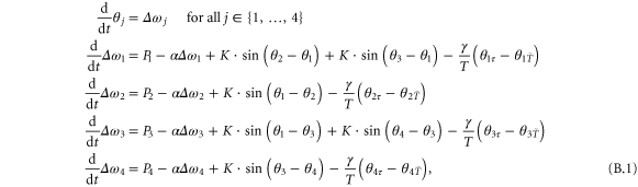
with  and
and  for all j.