

Abstract
Large-effect pigments, due to their strongly specular reflectance, produce a special visual texture known as sparkle. The use of these pigments in many industries (automotive, cosmetic, paper, architecture...) makes the control of this visual texture necessary. Sparkle measurands have been defined in this article, so that traceability of sparkle measurements can be provided by national metrology institutes or designated institutes. Some of them (Physikalisch-Technische Bundesanstalt, Eidgenössisches Institut für Metrologie, Cesky Metrologicky Institut and Consejo Superior de Investigaciones Científicas) have tested their existing measurement capabilities for the defined sparkle measurands, and their results are presented and thoroughly compared. Two possible sources of systematic error have been identified: inadequate illumination and collection solid angles, and an inadequate size of the virtual aperture used to assess the luminous flux reflected by the effect pigments. Finally, it has been shown that the measures correlate excellently with the sparkle visual data. The results shown in this research support the sparkle measurands defined here as adequate quantities for defining the standard measurement scale of sparkle claimed by industry.
Export citation and abstract BibTeX RIS

Original content from this work may be used under the terms of the Creative Commons Attribution 4.0 license. Any further distribution of this work must maintain attribution to the author(s) and the title of the work, journal citation and DOI.
1. Introduction
Sparkle, as defined by ASTM E284-17 Standard Terminology of Appearance[ 1] is 'the aspect of the appearance of a material that seems to emit or reveal tiny bright points of light that are strikingly brighter than their immediate surround and are made more apparent when a minimum of one of the contributors (observer, specimen, light source) is moved.' Large effect pigments, due to their strongly specular reflectance, produce sparkle, even when embedded in binders such as those used for coatings. The use of effect pigments in many industries (automotive, cosmetic, paper, architecture...) makes the control of this visual texture necessary. For instance, in the automotive industry, any differences between the car body and adjacent car parts are visible to the end customer, and they might need to present the same appearance, which is particularly important in the case of repair finishing [2]. It is convenient to accomplish the control by objective instead of subjective means, that is, by using physical measurements. The present technological state of imaging technology allows this, but until 2018 the only commercially-available instruments able to quantify sparkle were the BYK spectrophotometers for metallic colors (BYK-mac models) [3], which provide three sparkle indexes (area, intensity and general) for three different geometries (incidence angles of 15°, 45° and 75°, and a fixed collection angle of 0°). In 2018, the company X-Rite introduced two new portable multiangle spectrophotometers to the market (MA-T6 and MA-T12) [4], which use colour cameras to quantify sparkle. Both BYK and X-Rite have opted for defining their own sparkle scales, because to date there is no standard procedure for obtaining sparkle correlates from reflectance-related measurements. In consequence, the texture indexes provided by these instruments, although developed to be well-correlated with the visual experience, are not traceable to international standards. In the present situation, sparkle measurements from different instruments are not comparable. Without a standard measurement scale for sparkle, other companies might be reluctant to invest in new instrumentation, a competence that would improve the quality of sparkle measurements.
A standard measurement scale has to be defined, so that traceability can be provided by national metrology institutes (NMIs). Some of the NMIs (Physikalisch-Technische Bundesanstalt (PTB), Eidgenössisches Institut für Metrologie (METAS), Cesky Metrologicky Institut (CMI) and Consejo Superior de Investigaciones Científicas (CSIC), the latter as a designated institute) have developed photometric and image-based capabilities for measuring quantities related to sparkle. The results of a recently performed comparison are presented in this paper. The specific objective of this research work is to test these new capabilities, showing that these institutes can relate these quantities to their standards and that their measures are compatible, as a first step to providing traceability to sparkle measurements. Different measuring systems with different light sources, rotation mechanisms for the realization of angular geometries, and imaging luminance measurement devices were used. Luminance factor images were independently measured by each participating NMI, and the corresponding values were calculated from them, according to a measurement scale of sparkle. This measurement scale is under discussion by a technical committee of the International Commission on Ilumination (CIE), and its definition will be given below in this article. The data processing used to convert luminance factor images to values of sparkle quantities is common for all NMIs.
2. Methods
Sparkle quantities were calculated from luminance factor images of specially-selected samples, for which the value of each pixel corresponds to the luminance factor of the area of the sample imaged on that pixel. The definition of these quantities is based on the contrast between sparkle luminous points and the background in the luminance factor image, and on the accepted contrast threshold for luminous sources on darker backgrounds, which allows us to determine the visibility of a given sparkle luminous point. The defined sparkle quantities describe the density of the sparkle luminous points and the distribution of their visibilities.
Nine achromatic sparkle specimens, produced with different sizes and concentrations of effect pigments, were selected and their sparkle quantities measured by the goniospectrophotometers of PTB, METAS, CMI and CSIC, which were independently developed and have different designs. Each specimen was assessed at three different geometries, with low, medium and high aspecular angles (defined as the angular distance between the collection and the specular directions). The variation of the aspecular angle produces a variation in the observed sparkle because it varies the number of effect pigments oriented in a suitable position to be perceived as sparkle luminous points. Therefore, a total of 27 measurements (nine samples × three geometries) were compared in this work.
2.1. Measuring systems
2.1.1. CSIC.
Measurements are performed with the goniospectrophotometer GEFE, which is described in references [5, 6]. A sketch of the system is shown in figure 1.
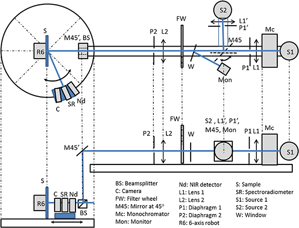
Figure 1. Sketch of the goniospectrophotometer GEFE at CSIC. (Top) Top view. (bottom) Side view.
Download figure:
Standard image High-resolution imageThe relevant features of the system are:
- 1.The irradiation system is fixed, whereas the sample and detector systems are mobile. The sample is held by a 6-axis robot-arm able to realize any required orientation relative to the incoming beam, while the detector can revolve around the sample.
- 2.A wide–band Xenon arc lamp (S2), which emits in the spectral range from 185 nm to 2000 nm, is used as light source.
- 3.The irradiation on the sample is uniform on a variable circle of a maximum diameter of around 3 cm.
- 4.The full angle of the illumination on the sample is 0.8°.
- 5.The measuring device is a CCD camera (QImaging, Rollera XR), with a Navitar Zoom 7000 18:108 mm objective zoom lens.
- 6.The field-of-view area of each pixel is 45
 45 .
45 . - 7.The full angle of collection is 2.5°.


2.1.2. METAS
Measurements are performed with the multi-angle reflectance setup (MARS), which is described in reference [7]. A sketch of the system is shown in figure 2.

Figure 2. Sketch of the Multi-angle Reflectance Setup (MARS) at METAS.
Download figure:
Standard image High-resolution imageThe relevant features of the system are:
- (a)The irradiation system can be placed into three illumination directions, whereas the detectors are fixed in ten collection directions (six in-plane and four out-of-plane). The sample system is mobile, to compensate for the sample's height.
- (b)A commercially available spectrally tunable light source with a wavelength range of 390 nm to 700 nm was used.
- (c)The irradiation on the sample is uniform.
- (d)The full angle of the illumination on the sample is 1.4°.
- (e)The ten measuring devices are 12-bit monochrome CMOS cameras.
- (f)The field-of-view area of each pixel is 42 42 .
- (g)The full angle of collection is 1°.


2.1.3. CMI.
Measurements are performed with the sparkle measurement facility at CMI. A sketch of the system is shown in figure 3.
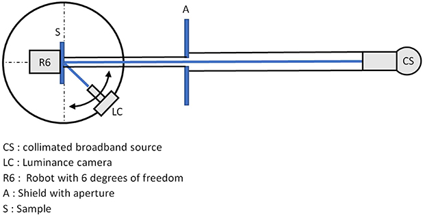
Figure 3. Sparkle measurement facility at CMI.
Download figure:
Standard image High-resolution imageThe relevant features of the system are:
- (a)The irradiation system is fixed, whereas the sample and detector systems are mobile. The sample is held by a 6-axis robot arm, able to realize any required orientation relative to the incoming beam, while the detector can revolve around the sample.
- (b)A halogen-based quasi-collimated light source was used.
- (c)The irradiation on the sample is uniform.
- (d)The full angle of the illumination on the sample is 2°.
- (e)The measuring device is a luminance camera (LMK5 Color) equipped with a CCD sensor (1380 pixels × 1030 pixels, 14 bits) and a V(λ) filter. The objective lens has a focal length of about 660 mm.
- (f)The field-of-view area of each pixel is 31 31 .
- (g)The full angle of collection is 4.2°.


2.1.4. PTB.
Measurements are performed with the goniospectrophotometer ARGON3D, which is described in reference [8]. A sketch of the system is shown in figure 4.
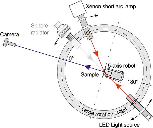
Figure 4. Sketch of the goniospectrophotometer ARGON3D at PTB.
Download figure:
Standard image High-resolution imageThe relevant features of the system are:
- (a)The collection system is fixed, whereas the sample and light sources are mobile. The sample is held by a 5-axis robot arm, able to realize any required orientation relative to the incoming beam, while the light source can revolve around the sample. A special double-sample holder allows a calibrated white standard with the sparkle sample under investigation to be manually interchanged by a perpendicular shift. This enables a prompt comparison of both samples in the same reflection conditions.
- (b)A wideband Xenon short-arc lamp and a LED light source were used as light sources. Therefore, since they have different spectral power distributions and irradiation full angles, it is considered that two different measuring systems were used at PTB.
- (c)The non-uniformity of the irradiation on the sample is typically less than 10 % in the central part of the sample (diameter 25 mm) for both lamps and around 25 % across a diameter of 50 mm in case of the Xenon lamp.
- (d)The full angle of the illumination on the sample is 1.8° for the Xenon lamp and 2.6° for the LED light source.
- (e)The measuring device is an SBIG STF-8300 CCD camera with an f = 210 mm Schneider-Kreuznach Componon-S objective.
- (f)The field-of-view area of each pixel is 24 24 .
- (g)The full angle of collection is 2.3°.


The descriptors most relevant for measuring sparkle are shown in table 1, for the five measuring systems. The meaning of the data in the last column ('Size of squared virtual aperture') is explained in subsection 2.4.
Table 1. Some relevant descriptors of the measuring systems.
| Spatial resolution of imaging system (µm) | Light source's full-angle (°) | Collection full-angle (°) | Side size of squared virtual aperture (µm) | |
|---|---|---|---|---|
| CSIC | 45 | 0.8 | 2.5 | 135 |
| METAS | 42 | 1.4 | 1.0 | 126 |
| CMI | 31 | 2.0 | 4.2 | 155.5 |
| PTB (LED) | 24 | 2.6 | 2.3 | 120.5 |
| PTB (Xenon) | 24 | 1.8 | 2.3 | 120.5 |
2.2. Description of sparkle samples
A set of nine achromatic samples (8 cm × 13 cm) was used in this study. These belong to the Effect Navigator set of 25 samples produced by Standox (see the photograph in figure 5) [9]. The samples in the set are composed of aluminum pigments, which are very parallel to the coating surface, and black absorption pigments. Each sample is labelled with an L number and an EN number, both of them varying from one to five, whose permutation makes 25 samples in total. We know by private communication that the L number is related to the concentration of effect pigments, whereas the EN number is related to the average size of the pigments in the sample, which is well-controlled and should have the typical values for aluminum pigments (0.5 µm - 200 µm). The sample set can be regarded as five groups of samples with fixed concentration of pigments and variable pigment sizes, or, reciprocally, as five groups of fixed pigment sizes and a variable concentration of pigments. We do not know the exact relation between the identification EN and L numbers and the real values. Visually, it is quite evident that the larger the L number, the lighter the sample, which means that the reflectance is related to the concentration of effect pigments. The larger the EN number, the more apparent the sparkle, as expected, since it depends on the luminous flux reflected by the effect pigments, which is proportional to the effect pigments' areas.
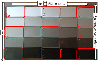
Figure 5. Standox Effect Navigator samples. The 9 samples used in this work are marked by red rectangles. No sparkle impression is observed, since the photograph was acquired under quasi-diffuse illumination. L and EN numbering in the sample labels ranks the samples according to pigment concentration and pigment average size, respectively.
Download figure:
Standard image High-resolution image2.3. Measurement geometries
The samples were measured at three measurement geometries, coincident with those in commercially available instruments. First, the collection angle ( ), defined with respect to the sample surface, was fixed at 0°, so that samples were always frontally assessed. Second, three different incidence angles with respect to the sample surface (
 ) were used: 15°, 45° and 75°. These three geometries provided three different aspecular angles (
 [10]). Notice that, since the effect pigments have orientations distributed almost parallel to the sample surface, the luminous flux specularly reflected by them, producing sparkle, is larger for low aspecular angles [11]. In consequence, three sparkle levels were expected to be found for each sample, one for each geometry.
2.4. Measurement of luminance factors of elementary areas
In order to measure sparkle, the spatial distribution of the luminance factor of the sample needs to be characterized as a first step. The most convenient way to do this is to use an imaging system able to acquire high-dynamic-range (HDR) sparkle images, since they usually have high contrast.
A dark-subtracted image of a uniformly irradiated sample (S) can be calibrated to provide luminance factors by comparison with the dark-subtracted image under the same geometrical conditions of a homogeneous diffuse reflectance standard of a known luminance factor in those conditions (W). The luminance factors (B) for each pixel are calculated as:
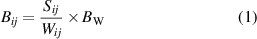
where Sij, Wij and Bij are the values of the (i,j)-pixels in S, W and B, respectively, and  is the luminance value of the diffuse reflectance standard, which is considered pixel independent.
Ideally,  and
and  should be acquired at exactly the same conditions of illumination and collection. However, in practice, the value of
  is only known for one (0°:45°) or a limited number of geometries. It is recommended that
  is acquired at (45°:0°), which according to the Helmholtz principle is equivalent to (0°:45°), and allows a frontal view of the sample to be acquired by the camera. In this case, to account for the variation of reflected luminous flux at other incidence angles
  , the previous equation is expressed as:
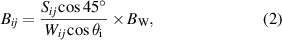
which holds as long as the source—sample distance is kept constant at different incidence angles. Notice that  provides the luminance factor at the field-of-view areas (
 ) of the pixels. However, those areas are not necessarily the most relevant elementary areas. The most convenient size of those elementary areas must contain most of the light attributed to a sparkle's luminous point. For the sake of simplicity, it can be morphologically defined as a square of pixels (a virtual aperture), with its side length measured in pixels (
 ). The image of a luminous point (modified by the point spread function (PSF)) is theoretically described as an Airy function, although in this practical case the rings are hidden by the background noise, and it can be regarded as a Gaussian distribution truncated by the finite size of the pixels. At the location of a sparkle luminous point, the maximum value of the pixels can be considered the centre of the elementary area. The square of pixels is radially expanded from this centre, and therefore (
 ) has to be an odd number.
The size of the elementary areas is calculated from the field-of-view area of a single pixel and the number of pixels within the defined elementary area ( ). The appropriate number of pixels making an elementary area can be obtained by analysing the profiles of some luminous points in the image B, so in general, the elementary area is dependent on the pixel size of the actual sample and may have to be be re-arranged for each sample. The size must be large enough to contain, for the majority of the luminous points in the image, those pixels whose values mostly represent the luminous flux reflected by the effect pigments.
The luminance factors of these elementary areas are the average of the pixel values composing the elementary areas in the luminance factor image (B). A practical procedure for calculating those luminance factors is as follows:
- 1.Find the pixel with maximum value in the image B.
- 2.Average the values of the pixels within the elementary area centered around that pixel. The resulting value is the luminance factor of that elementary area.
- 3.Obtain a modified image from B by setting the values of the pixels within that elementary area to zero.
- 4.Iterate steps (i) to (iii) with the subsequent modified images until all pixels have a value of zero. In the modified images, the pixels within the elementary area having a zero value are not considered. Also, the elementary areas where more than two thirds of the pixels have a zero value are neglected. By doing this, one avoids inclusion of the partial luminous fluxes of already-examined luminous points.
By applying this procedure, a distribution of luminance factors ( ) for the different elementary areas is obtained. As a result of this procedure, not only the values of the luminance factors of the elementary areas at the sites of sparkle luminous points, but also the luminance factors at sites with only background are obtained.
2.5. Definition of sparkle quantities
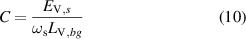
2.5.1. Contrast threshold.
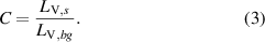
To define sparkle quantities, it is necessary to establish a criterion to identify the luminous points that are visible on the sparkling surface. The contrast at which a luminous source is distinguishable on a background was well determined by Richard Blackwell [12] by a visual experiment to determine a contrast threshold with 19 highly trained female observers aged 19–25. It is the largest and most authoritative study on contrast threshold. According to this study, the contrast threshold depends on the source luminance ( ), the background luminance (
 ), the size of the source, and the observation distance. In Blackwell's article, the contrast C is calculated as:
The contrast threshold  was defined as 'the contrast which was detected with a probability of 50 percent, due allowance having been made for chance success' [12]. Andrew Crumey, in the context of astronomy, has recently modelled Blackwell's experimental data [13]. According to this model, the contrast threshold can be expressed as:
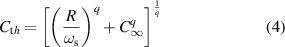
where q is a parameter dependent on  ,
,  is the solid angle subtended by the luminous source,
  is the asymptotic value of
  when
when  trends to infinity, and R is the proportionality value between
  and the inverse of
  when
when  is lower than a factor
  . This proportionality relation is known as Ricco's Law [13–15], and it is usually written as:

The maximum value of  for which it applies,
  , is sometimes called the Ricco area (although it has solid angle units). According to Crumey [13], its physiological interpretation is that the visual receptive field (corresponding to a number of receptor cells) sums the total energy received over its area, with a certain minimum energy being required in order to initiate a reaction. Both the Ricco area,
  , and the constant R become larger as the background luminance LV,bg decreases. Its significance is that luminous sources subtending less than the Ricco area are indistinguishable from point sources. It is assumed here that luminous points corresponding to sparkle subtend less than the Ricco area.
The more usual convention is to define the Ricco area,  , as the intersection of the asymptotes of the threshold curve [13, 16], that is, of the two equations resulting from equation (4) for
  trending to zero (
 ) and infinity (
 ). It results in a Ricco area as:
2.5.2. A contrast threshold for the luminance factors of elementary areas.
The luminance factor of an elementary area,  , is proportionally related to the illuminance,
  , produced on the eye by the luminous flux reflected by that elementary area, when it is observed under the same conditions for which its luminance factor was determined. Therefore, an illuminance contrast,
  can be defined for an elementary area (subscript e) as:
where the subscript 's' stands for luminous source, and 'bg' for 'background', and  is referred to the average luminance factor of those elementary areas in the images which do not contain luminous points.
  is the relative luminous flux reflected by an elementary area to the eye under those conditions, and
  is the increase of luminance factor due to the presence of a luminous point. Notice that, so defined, the illuminance contrast
  would depend on the size of the elementary area, simply because the illuminance at the eye depends on the elementary area in the case of the background (uniformly reflecting). However, it does not depend on it in the case of the luminous point (just a small area within the elementary area is reflecting). At this stage, standard conditions of observation need to be proposed. It is reasonable to rescale the ratio in equation (7) for elementary areas exactly filling the visual receptive field at the retina, or the Ricco area,
  . For this purpose, a standard observation distance
  , must be defined. It was selected as 0.5m, and it is the value used in this comparison. Then,
  is rescaled as
  as follows:
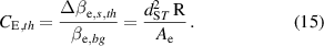
where  is the area of the elementary area (
 ) defined by the squared virtual aperture described in section 2.4.
It is very important to notice that the illuminance contrasts defined in equations (7) and (8) are different from the 'luminance' contrast defined in equation (3). When the elementary area includes a luminous point, its luminance factor is not proportionally related to its luminance, even if it is assumed that the camera acquisitions are luminance images. The reason is that the elementary area was defined in such a way that it overfills the luminous point, and consequently, it corresponds to a luminous flux measurement. However, the illuminance threshold ( ) can be deduced as follows.
The luminance of the luminous point in the elementary area can be expressed as:
As a result, equation (3) can be written as:
Now, Ricco's law (equation (5)) can be used to express equation (10) as the relation between the background luminance and the minimum illuminance that a luminous point needs to produce
to be visible at the eye,  , as:
, as:

On the other hand, analogously to equation (10), the background luminance is related to the illuminance at the eye produced by the elementary areas without luminous points as:

where  refers to the solid angle subtended by the elementary area. Since the illuminance contrast in equation (8) has been rescaled to have the elementary areas defined by the Ricco area,
  is
is  (with solid angle units). Then, according to equations (8), (11) and (12), it can be written as:
or:
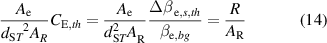
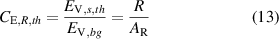
where  is by definition the contrast threshold when calculated from the illuminance at the eye produced by the elementary area defined by the virtual aperture, and
  is the contrast threshold when calculated from the illuminance at the eye produced by the elementary area defined by the Ricco area.
In equation (14),  is cancelled out, and the following expression is obtained:
Crumey's model provides an equation to calculate R for a given luminance background,  , as:
, as:
where:


and  must be expressed in cd/m2.
2.5.3. Determination of the luminance factor, , and the background luminance, .


Equations (15)–(16) allow the visibility of the luminous points on a background to be determined. This depends on the background luminance, which in turn depends on its luminance factor and the illuminance at the surface. The luminance factor of the background,  , can be taken as the luminance factor with the highest occurrence in the luminance factor distribution from the image B. To calculate the background luminance,
  , the illuminance at the surface (
 ) must be additionally known. A standard illuminance
  must be defined, related to the normal conditions of observation. Once
  and
and  are known, it is assumed that the background reflectance is Lambertian, in order to calculate the background luminance under standard conditions. In this case, the background luminance can simply be written as:
The assumption of Lambertianity does not introduce a considerable difference in the calculation of the contrast threshold, as long as the surface was quasi-Lambertian at the measuring incidence angles. Otherwise,  at standard conditions must be obtained by absolute measurements of luminance and illuminance.
2.5.4. Visibility of a sparkle luminous point in a single elementary area.
Equations (15)–(16) are used to calculate  , whereas equation (7) allows the calculation of
  for every elementary area. According to the definition, an elementary area with
  contains a visible luminous point. A correlate of the visibility of a luminous point,
  , can then be calculated as:
Thus, a luminous point in an elementary area is visible if  is larger than 0.
2.5.5. Definition of sparkle quantities.
- Sparkle visibility quartiles: The visibility of the luminous points (those with ) can be very diversely distributed, and it is convenient to use more than one parameter to characterize it. This distribution is quantified in a simple way using the quartiles 1, 2 and 3, denoted by , and , respectively.
- Sparkle density: The luminous point density, , is defined as the number of points per square millimeter that are visible ().


3. Results
There are some factors which have to be taken into account to understand the results. Although completely independent measurements of luminance factor images were carried out by CSIC, CMI, METAS and PTB, exactly the same measuring-system-independent algorithm was applied to the measurements to obtain sparkle visibility and density. Therefore, any variations in the results have to be related to the differences in the measuring systems, and not in the scale realization. Some of the most relevant differences in the measuring systems are summed up in table 1. They are mainly geometrical factors, such as the spatial resolution and the irradiation and collection full angles. Since the pixel fields of view of the imaging systems are different, the spatial analyses cannot be identical. Values between 120 µm and 160 µm were selected for the side of the squared virtual aperture defining the elementary area described in subsection 2.4. The selection of the virtual aperture is based on the largest length out of the PSF of the imaging system and the pigment particle size, and, ideally, it must be large enough to contain the signal from the sparkle luminous points in the image. The dependence on the spectral power distribution of the light source was assessed at PTB, where two light sources (a Xenon short lamp and a LED light source, see section 2.1.4), with similar irradiation full angles (1.8° and 2.6°, respectively), were used. Each NMI used its own strategy to obtain HDR images by combining acquisitions at different integration times. Only the two PTB datasets were processed with the same HDR algorithm.
The estimation of the uncertainty of the sparkle visibility quartiles and the sparkle visibility is complex, and non-conventional methods are required. For each sample and geometry there are many measures of visibility, (see equation (20)), one for each luminous point in the image, with a wide range of relative uncertainties. The uncertainty is larger for lower visibilities, for which the signals of the luminous point and the background are similar and the relative uncertainty of this signal ratio prevails over other uncertainty sources, those involved in the calculation of  , (see equation (15)). Those are the measurement of
  and
and  (through R in equation (16), and through
  in equation (19)). The relative standard uncertainty of
  is lower than 2.5 % in all the measurement systems, and the standard relative uncertainty of R is lower than 0.8 % in the worst case. Therefore, the relative standard uncertainty of
  is estimated as lower than 3 %. The uncertainty from other sources, as the incomplete directionality of irradiation or collection, the impact of using an insufficiently large virtual aperture, or of camera non-linearity, which is always an issue for HDR images composed with images having different integration times, are harder to estimate, and part of this study is to test if they are negligible for the measuring systems examined here.
The low-visibility luminous points, which are the majority, determine the quantities measured in this work ( and
and  ), and their uncertainty depends not only on the uncertainty of the visibility of individual luminous points, but also on the visibility distribution. The impact of the latter factor is assessed by examining the variation of different regions of the images, according to the procedure explained below.
A sparkle measurement taken on a relatively small area of a sample has to be representative of the whole surface. However, even when the measurement area contains a large number of sparkle points, some degree of inhomogeneity is unavoidable, as in any reflectance measurement, and different values are expected at different measuring regions on the surface. In this study, the sparkle quantities were assessed at nine different regions on the sample, each one with a measurement area of 3 mm × 3 mm. The relative standard deviation of the sparkle quantities across these regions reflects inhomogeneity and/or lack of spatial repeatability, where spatial repeatability refers to the closeness of the agreement between the results of measurements performed at the same time but at different positions in the image. Spatial repeatability is always worse than conventional temporal repeatability, since the former includes the same noise sources as the latter, and additional ones. This standard deviation across different regions, hereafter called as 'inhomogeneity' for simplicity, will be regarded as the estimation of the total uncertainty of each measuring system when assessing the compatibility of the measurements in the comparison. This inhomogeneity includes the impact of the other uncertainty sources above mentioned, except from  , whose impact is much lower. The compatibility study in this comparison is important in order to find out if additional relevant error sources in the measuring systems need to be identified.
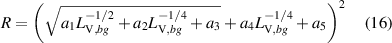
Examples of luminance factor images from the participating institutes are shown in figure 6, corresponding to sample L3 EN3 at an incidence angle of 45°. The images present differences in the apparent size of the luminous points, which is likely due to the cameras' PSF differences. The positions of the luminous points are not coincident, since the measuring position was not so tightly controlled (the measurement area was approximately centered at the center of the sample). Measurements with a BYK-mac instrument showed that the sparkle indexes did not present much larger reproducibility (measures at different position and orientation of the sample) than repeatability (measures at exactly the same position and orientation of the sample) in the set of samples
studied. The reader should notice that the similarity between images is not the key sparkle quantity to be compared. The key quantities for comparison are the median of the sparkle visibility ( ) and the sparkle density (
 ). Although these values are calculated from the images, low similarity between the images would not be incompatible with a good match in terms of sparkle visibility and density. A good match is possible as long as the luminous flux reflected by individual effect pigments for given geometrical conditions can be assessed from the image.
Figure 6. Examples of measured luminance factor images for sample L3 EN3 at  . All images are from the central area of the sample, but the exact position is not controlled at this small scale.
Download figure:
Standard image High-resolution imageIn addition to sparkle visibility and density, the background luminance factor background ( ) is the third quantity to be compared. Averages for the three quantities across nine regions of the sample are given in figure 7, whereas the standard deviations for the nine samples, the four institutes, and with an incidence angle
  of 45°, are shown in figure 8. As is shown in figure 7, the averages of the sparkle densities,
  , in figure 7(c), present larger discrepancies between institutes than the averages of the median sparkle visibility,
  , in figure 7(b). It is interesting to note that METAS's values for
  are always the highest ones. That might be related to its lowest combined measuring full angle (the maximum full angle among collections and illuminations, see table 1). The value of this combined measuring full angle affects the sparkle visibility when the reflections from effect pigments are so directional that they do not completely fill the collection aperture. Regarding the sparkle density figure 7(c), it is noticeable that METAS and PTB generally obtained larger values than CSIC and CMI. This might be due to the relatively smaller size of their virtual apertures (126 µm and 120.5 µm vs. 135 µm and 155.5 µm, see table 1). The size of the virtual aperture limits the maximum number of elementary areas to be assessed within a given surface. In addition, if the virtual aperture is too big, multiple sparkle points can be accounted for as one, whereas if it is too small, one sparkle luminous point might be accounted for as two separate ones. Both effects could explain part of the observed differences of METAS and PTB (larger sparkle densities and smaller virtual apertures) with respect to CSIC and CMI (smaller sparkle densities and larger virtual apertures).
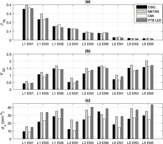
Figure 7. Averages across nine regions on the sample of (a) background luminance factor ( ), (b) median of sparkle visibility and (c) sparkle density for the nine samples, the four institutes, and with an incidence angle
  .
.
Download figure:
Standard image High-resolution image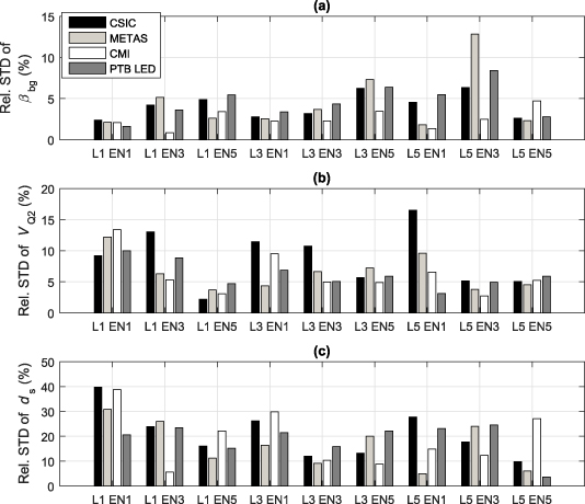
Figure 8. Relative standard deviations across nine regions of the sample, of (a) background luminance factor ( ), (b) median of sparkle visibility and (c) sparkle density, for the nine samples, the four institutes, and with an incidence angle
  .
.
Download figure:
Standard image High-resolution imageFrom the relative standard deviations shown in figure 8 it is not possible to identify systematic differences among institutes. These variations are much smaller for  (usually lower than 5 %) than for
  (with an average of around 5 %) and
  (with an average above 10 %). The discrepancy among institutes indicates that the variation is mainly due to the limitations of the methodology and not to variations across the sample.
The averages across the five datasets (CSIC, CMI, METAS, PTB LED and PTB Xe) of  and
and  are represented in figure 9, where each plot corresponds to a measurement geometry (
 = 15°, 45° and 75°). The error bars represent the standard deviation of the sparkle quantities across the five datasets, showing the disagreement among measuring systems.

Figure 9. The average values of the measurements of the five datasets (CSIC, METAS, CMI, PTB LED and PTB Xe). Error bars represent the standard deviation of the sparkle quantities. The reader should notice the different scale of the graphs.
Download figure:
Standard image High-resolution image4. Discussion
The trends of the data represented in figure 9, from nine samples providing a large range of sparkle level, are consistent with the expectations. The lower the incidence angle ( ), the larger both
  and
and  . This is expected, because low incidence angles correspond in this case with low aspecular angles, which should favour sparkle (see final comment in subsection 2.3). Samples with larger pigment sizes (larger EN-numbers) should produce more sparkle, since more luminous flux is reflected specularly. On the other hand, samples with higher pigment concentration (lower L-numbers) should produce less sparkle, since they have larger background luminance. Both statements are proven correct when observing the trends of
  and
and  .
.
The results indicate a clear relation between  and
and  , although it is not linear. Whereas
  seems to be able to grow up to a non-defined upper limit,
  apparently reaches a saturation at around 50 mm−2 for large values of
  . This value of sparkle density saturation results in a mean distance between sparkle luminous points of around 142 µm, which is close to the size of the virtual apertures used in the measurements (see table 1). It is likely that the identification of the sparkle density saturation must be regarded as a limitation of the measuring systems, but also of the measurement itself, due to the clustering of the sparkle luminous points at very large levels of sparkle.
So far, we have shown the coherence of the combined result obtained from five different measuring systems. However, the aim of this work is mainly to evaluate the present capabilities of NMIs to measure sparkle-related quantities, and to identify possible ways for improvement. In order to find overlooked uncertainty sources, the compatibility of the measurements was studied, under the assumption that the total uncertainty is properly estimated from the variation between different regions on the sample's surface. A compatibility index was calculated for each single measure. There are 2 sparkle quantities ( and
and  ), 5 measuring systems (CSIC, METAS, CMI, PTB LED and PTB Xe), 9 samples, and 3 measurement geometries (
 ,
,  , and
, and  ), making a total of 270 measurements with their corresponding compatibility indexes [17], calculated as:
where Q is the sparkle quantity ( or
or  ),
),  denotes the comparison reference value (CRV) of Q( average values represented in figure 9), U(Q) is the expanded uncertainty of Q exclusively due to variations at different regions on the sample's surface, and finally
  is the expanded uncertainty of
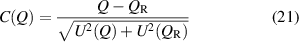
  , which is calculated as the standard deviation of the mean across institutes. An absolute value of C larger than 1 represents an incompatibility within a 95 % confidence interval. Notice that, in order to evaluate systematic errors, the sign is not neglected in the definition of C. However, it was removed in the general overview shown in figures 10 and 11 by taking the absolute values.

Figure 10. Absolute values of the compatibility indexes obtained in the comparison of the median sparkle visibility,  .
.
Download figure:
Standard image High-resolution image
Figure 11. Absolute values of the compatibility indexes obtained in the comparison for sparkle density,  .
.
Download figure:
Standard image High-resolution imageCompatibility values for  are shown in figure 10 for the five evaluated measuring systems, the nine samples, and the three geometries, while the same representation for
  is given in figure 11. Both figures show that the compatibility is rather independent of sample or geometry. However, there is some dependence on institute, as in the case of METAS's data, with excellent compatibility for
  and low compatibility for
  .
.
The compatibility data were plotted in a  –
– ) diagram (figure 12) to better identify possible systematic biases of the measuring systems. The values within the central square represent combinations of sample and geometry whose
  and
and  measurements are both compatible with the general result. They represent 57 % of the total number of measurements. Those measurements only compatible in
  are lying within the vertical -1 and 1 lines, whereas the horizontal -1 and 1 lines enclose those measurements only compatible in
  (75 % and 73 %, respectively). Almost one tenth of the measurements are incompatible in both
  and in
  . These incompatible measures are useful to identify systematic errors and to improve the measuring systems. There are two interesting observations:
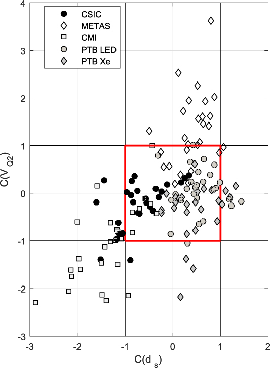
Figure 12. Compatibility data. The values within the central square represent combinations of sample and geometry whose  and
and  measures are both compatible with the general result.
Download figure:
Standard image High-resolution imageFirstly, the incompatibilities of METAS's values are always positive in  , whereas those from CMI are always negative. This might be explained if the sparkle is more visible in METAS's images and less in CMI's images with respect to the other institutes'. This is precisely the effect that should be caused by different illumination and collection combined full angles: the larger they are, the less visible the luminous points. This hypothesis can be evaluated by looking at figure 13, where the degrees of equivalence (DOE, relative deviation with respect to the CRV) of
  measures are shown as a function of their CRV. Each dataset corresponds to a different measuring system, which is specified in the legend along with the maximum combined full angle (cfa). It can be observed that the average value of
  depends on the measuring system, with METAS having the largest positive deviation, and CMI the largest negative one, which is coherent with their combined full angles (1.4° vs. 4.2°). This value is very similar (between 2.3° and 2.6°) in the case of the other measuring systems, whose
  measures are compatible with the complete comparison in 91 % of the cases.
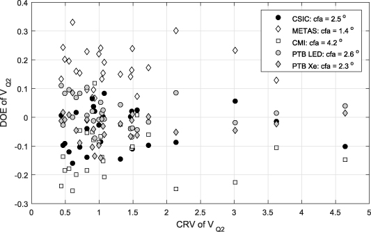
Figure 13. Degrees of equivalence of  measurements as a function of their comparison reference values (CRV).
Download figure:
Standard image High-resolution imageSecondly, the incompatibilities of both CSIC's and CMI's measures are always negative for  . This should be related to an underestimation in the counting of sparkle luminous points, which might be related to too large a size of the virtual aperture. This hypothesis can be evaluated by looking at figure 14, where the degrees of equivalence of
  are shown as a function of their CRV. Each dataset corresponds to a different measuring system, which is specified in the legend along with the size of the virtual aperture, as reported in table 1. It can be observed that the average value of
  depends on the measuring system, having CMI the largest negative deviation, and CSIC the second largest. This is consistent with their virtual aperture sizes (155.5 µm and 135 µm, respectively). In the case of the other measuring systems, whose
  measures are compatible with the complete comparison in 90 % of the cases, the virtual aperture sizes are smaller (between 120.5 µm and 126 µm). It should be mentioned that CMI might have provided a higher spatial resolution by selecting a virtual aperture size of 93 µm, but that proved to be too small, producing a worse compatibility. Thus, it is important to recommend a virtual aperture size for measuring sparkle in effect coatings. According to the results of this study, a value between 120 µm and 125 µm might be suitable.

Figure 14. Degrees of equivalence of  measurements as a function of their comparison reference values (CRV).
Download figure:
Standard image High-resolution imageNo important differences were found in the results of PTB's two measuring systems. The one with the wideband Xenon short-arc lamp obtained three values with unusually large incompatibility. All three of them were measured at the geometry  = 75°, using samples with high sparkle. The two less-compatible values presented very large homogeneity. No clear conclusions could be drawn concerning the effect of the light source on the measurement of sparkle.
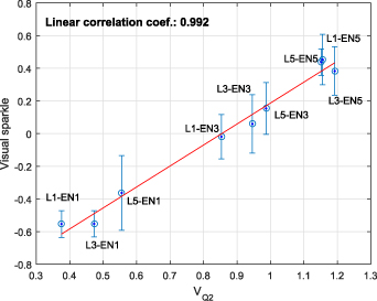
The sparkle quantities defined and measured in this work are based on the contrast threshold of the human vision system, and they should be directly or indirectly related to the visual experience of sparkle. This relationship was evaluated by a psychophysical method, where the measures of sparkle quantities shown here were compared with visual data obtained at the University of Alicante. A very close linear correlation was found between sparkle visibility and the visual data, with a linear correlation coefficient of 0.992. This relation and the linear fitting results are shown in figure 15. The error bars represent the inter-observer standard deviation for each specimen. For reference, notice that the linear correlation coefficient with BYK-mac's general sparkle index is 0.963.
Figure 15. Relation between visual sparkle and  . The error bars represent the inter-observer standard deviation.
Download figure:
Standard image High-resolution image
The coefficient's good correlation with the visual data, the reproducibility of its measurement by different instruments, its well-defined relation with the radiometric quantities involved and observation conditions make the sparkle visibility defined in section 2.5 an excellent candidate to be the key quantity for a standard measurement scale.
5. Conclusions
The measurement of the sparkle quantities of nine samples with effect coatings at three different geometries was independently carried out by three different national metrology institutes (PTB, METAS, CMI), and one designated laboratory (CSIC), in order to evaluate their capabilities for measuring sparkle, as a first step towards providing traceability. For the first time, a publicly accessible definition of sparkle measurands (sparkle visibility and sparkle density) has been presented. This measurement requires methods which are not well-established yet, such as those for using imaging systems as optical radiation detectors in inhomogeneous environments. The measuring systems described here, with different light sources, rotation mechanisms for realizing angular geometries, and imaging luminance measurement devices, have provided compatible results in the measurement of the sparkle quantities, which allow the samples to be clearly distinguished and described in terms of sparkle visibility and density, and the effect of the aspecular angle to be quantified. Two possible sources of systematic errors have been identified: inadequate illumination and collection solid angle angles, and inadequate size of the virtual aperture used to assess the luminous flux reflected on the effect pigments. The size of this virtual aperture is dependent on the kind of sample, and has to be selected according to the average apparent size of the luminous points in the images. The agreement, and not only correlation, of measures of sparkle quantities by different instruments is key to providing traceability of this measurement. The presented results go far beyond the state of the art, where, so far, no attempt has been made to measure the same quantities. The reason is that different scales have been independently defined for each existing commercial instrument, and therefore they are not comparable. The sparkle quantities defined in this work are instrument-independent, and they are based on the widely-accepted contrast threshold of the human visual system. This allows not only the visibility of the sparkle luminous points to be expressed from reflectance quantities, but also as a function of the observation distance and the illuminance, whose impact in sparkle perception has been clearly stated in visual studies, but which so far has not been considered in existing sparkle indexes. In addition, it has been shown that the defined sparkle visibility correlates excellently with the sparkle visual data. These considerations and the measurement reproducibility shown in this work, make the proposed sparkle quantities ideal for defining the standard measurement scale of sparkle claimed by industry.
Acknowledgments
This article was written within the EMPIR 16NRM08 Project 'Bidirectional reflectance definition' (BiRD). The EMPIR is jointly funded by the participating countries within EURAMET and the European Union. Some of the authors (Instituto de Óptica 'Daza de Valdés') are also grateful to Comunidad de Madrid for funding the project S2018/NMT-4326-SINFOTON2-C.