
Abstract
Objective. Recent studies have provided evidence that temporal envelope driven speech decoding from high-density electroencephalography (EEG) and magnetoencephalography recordings can identify the attended speech stream in a multi-speaker scenario. The present work replicated the previous high density EEG study and investigated the necessary technical requirements for practical attended speech decoding with EEG. Approach. Twelve normal hearing participants attended to one out of two simultaneously presented audiobook stories, while high density EEG was recorded. An offline iterative procedure eliminating those channels contributing the least to decoding provided insight into the necessary channel number and optimal cross-subject channel configuration. Aiming towards the future goal of near real-time classification with an individually trained decoder, the minimum duration of training data necessary for successful classification was determined by using a chronological cross-validation approach. Main results. Close replication of the previously reported results confirmed the method robustness. Decoder performance remained stable from 96 channels down to 25. Furthermore, for less than 15 min of training data, the subject-independent (pre-trained) decoder performed better than an individually trained decoder did. Significance. Our study complements previous research and provides information suggesting that efficient low-density EEG online decoding is within reach.
Export citation and abstract BibTeX RIS

Content from this work may be used under the terms of the Creative Commons Attribution 3.0 licence. Any further distribution of this work must maintain attribution to the author(s) and the title of the work, journal citation and DOI.
1. Introduction
Disentangling separate speech streams in multi-speaker environments is a perceptually complex task for normal hearing individuals and can be compromised by hearing loss (Shinn-Cunningham and Best 2008) and aging (Ruggles et al 2012, Shinn-Cunningham et al 2013). The most engaging chat may be difficult to follow in the presence of other competing speech streams. While spatial, temporal and frequency cues help to identify and disentangle concurrent speech streams, a deficiency in cue processing at any part of the auditory pathway may lead to reduced attentional selection and low speech intelligibility (Shannon et al 1995). Accordingly, developing assistive devices helping individuals to follow an attended speech stream in complex listening situations is a desirable goal. Normal hearing individuals rely on spatial and spectro-temporal cues to separate speech streams and other sounds into individual auditory objects (Ihlefeld and Shinn-Cunningham 2008, Ding and Simon 2012a, Simon 2014). Spectral and temporal cues, like pitch, timbre and intensity, are predominantly synchronized to the speech rhythm. This knowledge sparked the idea that cortical responses to speech may be correlated with the (delayed) temporal amplitude envelope carrying this speech rhythm (Aiken and Picton 2008, Ding and Simon 2014).
Recently the idea of envelope based speech reconstruction from cortical recordings emerged. Single-trial intracranial recordings from the auditory cortex were utilized for the purpose of explaining neural encoding mechanisms (Pasley et al 2012). This study successfully developed a reconstruction model for low spectro-temporal modulations of individual words and sentences, corresponding to formants and syllables. An attention-driven top-down effect on cortical speech envelope representation may be crucial in speech perception research (Mesgarani and Chang 2012, Horton et al 2014). The attention effect was investigated with intracranial data by expanding the results found in low frequencies to the high gamma band (Zion Golumbic et al 2013). However, the gamma band suffers from a low signal-to-noise ratio when studied with non-invasive electroencephalography (EEG). Other groups exploited the low frequency range (1–8 Hz) for the reconstruction of attended and unattended speech in two speaker scenarios, using either high-density magnetoencephalography (MEG) (Ding and Simon 2012b) or high-density EEG (O'Sullivan et al 2014), as it is known that this frequency range corresponds to the spectrum of speech envelopes (Zion Golumbic et al 2012). These two studies confirmed that attended and unattended speech were differentially represented in EEG/MEG, with the cortical response to unattended speech being suppressed and the response to attended speech being amplified. In the EEG study of O'Sullivan et al, both speech streams were represented in the EEG albeit to a different extent. The authors speculated that the latency at which the attended speech became dominant may suggest the lag the attended stream was encoded into working memory. However, while the temporal envelope reconstructions achieved with non-invasive studies, such as MEG and EEG, cannot be used to reproduce intelligible speech, they seem to convey sufficient information to distinguish between attended and unattended speech streams. By correlating the EEG-based reconstruction signal with the original speech stimuli envelopes, a very high decoding accuracy (i.e., the percentage of accurately classified trials) was reported (O'Sullivan et al 2014). Accordingly, non-invasive measures may provide sufficient information to infer which of several speech streams a listener currently attends to. Making this information readily available in near real-time may, for instance, constitute a valuable input signal into a new generation of hearing devices and is of interest in basic auditory neuroscience to test which speech features are best represented on a cortical level and contribute to stream segregation.
Our first goal was to conceptually replicate the work of O'Sullivan et al (2014). Secondly, we investigated how decoding accuracy relates to spatial sampling accuracy, that is, the number of EEG channels used. The motivation for this analysis was that mobile, motion-tolerant EEG is possible with relatively low-density, low weight, wireless and head-mounted EEG systems (Debener et al 2012, De Vos and Debener 2014, De Vos et al 2014a, De Vos et al 2014b). Accordingly, to quantify the relationship between channel count and decoding performance we adopted a channel selection iterative procedure established previously in a different context (Zich et al 2014). Iteratively, in the offline analysis of high-density EEG recordings the EEG channel carrying the least contribution to decoding accuracy is identified and eliminated and this procedure is repeated from 96 down to very few EEG channels. This procedure identifies both the optimal number and optimal position of EEG channels per subject, and it provides information about the minimum number of channels needed on average for attended speech decoding as well as the best across subject placement of electrodes on a cap. And thirdly, a long-term goal of near real-time decoding would benefit from a short calibration period, and a stable decoding performance over longer periods of time. Aiming towards this goal, we used chronological calibration applied to incremental amounts of training data to investigate the relationship between amount of training data and decoding accuracy. Moreover, we built a subject-independent decoder based on information from all other subjects and contrasted the decoding performance to an individual decoder. A subject-independent decoder returning above chance-level performance would allow immediate presentation of feedback, during an initial individual training period. Accordingly, we investigated how much data is needed to recalibrate the decoder for a new user as compared to using a subject-independent one.
2. Methods
2.1. Participants
Twelve adult participants between the ages of 21 and 29 took part in this study. Eleven participants were consistent right-handers, one was a consistent left-hander. Participants reported no present or past neurological or psychiatric conditions and normal hearing. All participants were native German speakers. Prior to the experiment all participants signed informed consent and afterwards received monetary reimbursement. The study was approved by the local ethics committee.
2.2. Stimuli
Two works of fiction ('A drama in the air' by Jules Verne and 'Two brothers' by Grimm brothers) were narrated in German language, each by a different sex speaker. Silent periods exceeding 0.5 s were truncated to 0.5 s in order to keep listeners attention and minimize the possibility of switching attention to another story. Speech streams were spatially separated by imposing interaural level differences such that one speaker was located at 30° to the left and the other 30° to the right side of the listener. Both speech streams were sampled with a frequency of 48 kHz and stimuli were presented binaurally via insert earphones (E-A-RTONE 3A). Sound was presented via a Tucker Davis Technologies programmable attenuators (PA5) and controlled by the Neurobehavioral Systems Presentation software. Sound level was individually adjusted to a comfortable level.
2.3. Procedure
Participants were instructed to attend to one out of the two concurrent speech streams presented. Speakers location and speaker attention were balanced out across participants, that is, six participants attended to the male speaker and six to the female speaker. Half of the participants attended the stream perceived as coming from the right location and the other half to the stream coming from the left location. Participants were instructed to keep their eyes open, minimize blinking and keep their gaze straight ahead. The stimulus presentation lasted 48 min in total and was divided into five sessions (the first four lasted 10 min and the last session 8 min). Presentation of the story was interrupted by four inter session breaks. During the breaks participants were required to fill out a questionnaire consisting of eight multiple-choice questions, four of which pertaining to the story they were attending to and four pertaining to the unattended story. Participants could choose to leave a question unanswered if they did not know the answer. Additionally, participants were strongly discouraged from guessing the answer to any question.
2.4. EEG recordings and preprocessing
EEG data were acquired in a sound shielded room while participants were seated in a comfortable chair. Data were collected with a BrainAmp system (BrainProducts GmbH, Gilching, Germany) and use of equidistant infra-cerebral 96 channel Ag/AgCl electrode caps, provided from Easycap (www.easycap.de). Data was referenced to the nose-tip and recorded with a sampling rate of 500 Hz (analog filter settings 0.0153–250 Hz). Data pre-processing was performed offline, following the steps described in O'Sullivan et al (2014) using EEGLAB (Delorme and Makeig 2004) and MATLAB (Mathworks Inc., Natick, MA). Specifically, EEG data were re-referenced to a common average reference, band-pass filtered between 2 and 8 Hz and subsequently downsampled to 64 Hz. Speech envelopes were obtained using a Hilbert transform of original, individual speech streams, followed by low-pass filtering at 8 Hz and downsampling the resulting signal to 64 Hz.
2.5. Speech reconstruction
Speech reconstruction was performed as proposed by O'Sullivan et al (2014). Briefly, the preprocessed EEG recordings were segmented into trials of 60 s duration, resulting in 48 trials per subject (N = 48). In order to computationally include all potential lags between presented stimulus and respective cortical responses indicated by previous studies, the EEG segments were zero padded on the left side. Time lags containing information about attended speech streams were searched between 0 and 300 ms using a window width of 30 ms. The decoder of the attended speech g was estimated on the segmented and zero padded EEG data, presented as R(n*(d + 1),t), where n is a number of EEG channels and d the number of utilized discrete time lags, and the corresponding envelope of an attended speech stream S(1,t) using a regularized least square estimation method

The regularization parameter λ was empirically determined, while the regularization matrix M was given as follows:

The decoder was trained on each trial separately and consisted of EEG channel reconstruction weights at individual time lags within a range specified by zero padding. Each of the 48 decoders trained per subject can be interpreted as a single spatio-temporal filter designed for 60 s of data, providing information about how much each scalp channel contributes to processing of an attended speech stream. The decoder used for the reconstruction of one trial was obtained by averaging the reconstruction weights of all decoders trained on all other trials of the same subject, following a classical cross-validation approach. Stimulus reconstruction for each trial  was obtained by convolving the decoder with the corresponding EEG segment

Reconstruction performance was evaluated by means of parametric correlations between the reconstructed signal with the envelope of the attended and the envelope of the unattended speech stimulus. The attended speech stream was correctly identified when the correlation with the attended stream was higher than the correlation with the unattended speech stream envelope, regardless of the magnitude of the correlation. Decoding accuracy was then defined as the percentage of accurately reconstructed trials for each subject. Time lag intervals with highest decoding accuracies for all subjects and physiologically plausible decoder topographic patterns compatible with contributions from auditory cortical areas were then used for further analysis.
After this initial analysis, decoder was retrained on chosen narrow time lag interval for all subjects. Stimulus reconstruction was performed using these decoders. Decoding accuracies for narrow time lag interval were obtained and compared to the reported findings from O'Sullivan et al (2014).
2.6. Electrode reduction
Electrode reduction from the initial electrode set was performed individually for each subject using an iterative backward elimination algorithm. In the first iterative step a decoder for attended speech was trained on all 96 channels available, as described above. At the end of the first iteration, the decoding accuracy achieved by a particular subject was calculated and the corresponding reconstruction weights from all 48 decoders were averaged. The electrode with the lowest average reconstruction weight was then determined and removed from the next iteration. This step was repeated for all twelve subjects and from 96 down to 1 channel as follows: the decoder reconstruction weights were recalculated on the remaining channels and the decoding accuracy resulting from the newly trained decoders was assessed using leave one out cross-validation. Note that the time lags taken into consideration were kept constant across subjects and iterations. For each layout size this analysis indicated the most efficient electrodes for every participant. Mean decoding accuracy across all participants for each iteration step was then evaluated, as well as the relative frequency of the remaining channels. To validate the obtained results of the main analysis and assess the applicability of this method, we calculated the average decoding accuracy across all subjects using the fixed 24 electrode layout for all subjects, the configuration of which was determined using the most frequently selected channels from the previous analysis.
2.7. Chronological validation
In order to simulate an online experiment, we also evaluated decoding accuracy when only a first part of all trials is used. For each subject 30 decoders were obtained, each based on different sizes of data used. Specifically, each decoder was trained on a limited number of first trials recorded from one subject, ranging from 1 to 30 min. Assessment of decoder accuracy was performed on the remaining trials. Note that for this reason the validation sets were not equal sized and thus small variations could be expected. The accuracies achieved by different subjects at specified recording time points were averaged and the mean accuracy across all subjects was considered. In the following, decoders trained and chronologically validated in this approach will be referred to as individual decoders.
2.8. Pre-trained decoder
Applying the leave-one-out logic to across subjects, we defined a pre-trained decoder as the mean of all decoders trained on all participants except for the one whose trials were being classified. Note that this procedure included decoders obtained from participants that attended to the other speech stream. The benefit of a pre-trained decoder was expected to be limited to early recording durations, until a decoder trained on previous trials of a particular subject has 'seen' enough data to be robust. To obtain a decoding accuracy comparable to that of the individual decoder at all specified recording time points, we performed validation of a pre-trained decoder on the same datasets as the ones the corresponding individual decoder was validated on. We computed the average decoding accuracy across all subjects which resulted in 30 mean accuracies, one at each recording time point.
3. Results
3.1. Speech reconstruction
Analysis of the questionnaire data showed that all participants followed the instructions and attended to the indicated speech stream. On average, participants answered correctly to 91.7% of the questions pertaining to the attended story and only to 5% of questions pertaining to the unattended story. Some questionnaire responses indicated that few participants recognized certain words from the unattended story, but this rarely resulted in a correct response to a question about the content of the unattended story.
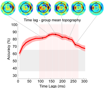
Figure 1. Group average decoding accuracy with standard error of the mean for time lags ranging from 0 to 300 ms, with a window of 15 ms. Topographies show spatial distribution of electrode reconstruction weights around specific time lags, averaged within the time lag range indicated by vertical red shaded areas. Gray shaded area represents chance-level.
Download figure:
Standard image High-resolution imageAnalysis of average decoding accuracies across all subjects through 15 ms time lags from 0 to 300 ms showed that accuracies reached highest values when time lag intervals from 130 to 220 ms were used (figure 1). After 300 ms post-stimulus mean decoding accuracy dropped below chance-level. Interestingly, group average decoder maps showed clear patterns of bilateral temporal topographies consistently for all time lags up to 300 ms. For the three early lags the decoder weights were right-lateralized, whereas for the three later lags they were clearly left-lateralized.
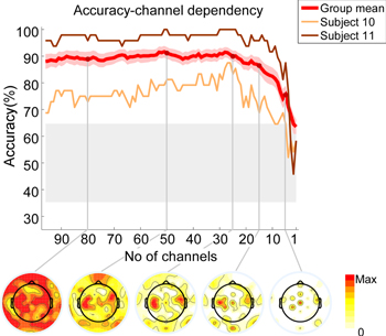
Figure 2. Group mean decoding accuracies with standard error of the mean for decreasing number of channels from 96 to 1. Single subject results are given for the worst and one of the best performing subjects. Topographies show the relative frequency of remaining channels for indicated layout size. Gray shaded area indicates chance-level.
Download figure:
Standard image High-resolution imageIncluding those four latency windows indicated by the topographical inspection as most relevant, we trained a decoder using 150–220 ms time lag interval. Validation of a decoder trained on this narrow time lag interval resulted in a group mean accuracy of 88.02% (range 68.75–100%). Eleven out of twelve participants performed significantly above chance-level, which was determined as 64.7% based on a binomial significance threshold.
3.2. Electrode reduction
Figure 2 shows the result of the decoder performance when a subset of electrodes was used, decreasing from 96 to a single electrode. On average, subjects performed well above chance-level if more than five channels were used for the analysis. For more than 25 electrodes there was no clear improvement in decoding accuracy, that is, the decoding accuracy remained robustly above 85% regardless of whether 96 or 25 electrodes were used, or any number in between. A clear decline in decoding accuracy was observed for the lowest performing subject with less than 25 electrodes, and for the best performing subject for less than 12 electrodes. Notably, applying an individualized electrodes setup comprising 15 electrodes resulted in an average decoding accuracy of 87%. Lowering the density even further to five electrodes revealed an average decoding accuracy of 74.1%, which was still well above chance-level. A similar pattern was observed in all individual subjects, not only in the worst and best subjects illustrated. While inter-subject variability was substantial all subjects performed above chance-level with 10 or more electrodes, while two achieved very high performance (>90%) with as few as six electrodes included.

Figure 3. Comparison of mean decoding accuracies achieved with individual decoder and with pre-trained decoder at specific training intervals ranging from 1 to 30 min. Respective standard deviations are also shown. Gray shaded area indicates the chance-level.
Download figure:
Standard image High-resolution image
Frequency map calculation of the selected channels at different iteration steps revealed a bilateral temporal distribution, compatible with contributions from brain areas known to process auditory signals. These areas were clearly represented on medium density subsets (25–50 electrodes), although also with clear influence from posterior brain sites. By using the most frequently chosen 24 electrodes for all single subjects, a decoding accuracy of 86.6% was achieved, which is close to the decoding accuracy achieved for 24 channels used based on individualized layouts (90.1%). This suggested that use of a pre-determined, standardized channel layout did not result in a relevant loss of decoding accuracy.
3.3. Chronological validation
Using an individual decoder trained on the first minute data only and validated on the remaining 47 min resulted on average in a below chance-level mean accuracy. When the duration of the training interval was increased, the individual decoder improved in performance (figure 3). After 8 min, 10 subjects performed above chance-level, with mean accuracy of 78%. When a relatively low number (<15) of chronologically preceding trials was used for decoder training, the mean decoder accuracy across all subjects was above chance. Beyond 15 trials, accuracy constantly increased with an increasing amount of data used for training. However, for low performing subjects the individual decoder did not perform above chance-level within 15 min of training data. All subjects showed a distinct increasing trend as the training set became larger, resulting in a more reliable individual decoder performance after inclusion of 15 or more minutes for decoder training (mean accuracy 82.6% at 15 min). With training sets consisting of 21 min of EEG recordings only one subject remained below chance-level. The best performing subject on the other hand achieved perfect classification after only 8 min and one half of the recorded participants showed a very fast learning effect. Performance of all subjects improved by the end of the 30th minute, with accuracies ranging from 56 to 100% (mean accuracy 84.7%).
3.4. Pre-trained decoder
The mean decoding accuracy achieved with a pre-trained decoder at specified intervals is shown on figure 3 as well. The pre-trained decoder showed stable performance at approximately 81% accuracy throughout the trials, while the fluctuations illustrated were based on different sizes for the validation sets. Based on the group mean result, the individual decoder reached the pre-trained decoder efficiency after 14 min of recording and from that moment on resulted in higher performance. In two subjects the pre-trained decoder resulted in better classification then the chronological individual approach even after 30 min training. In all remaining subjects the individual decoder outperformed the pre-trained decoder.
4. Discussion
This study explored whether an existing speech decoding procedure could be replicated, and identified constrains that should be considered for future online scenarios. One possible application for this method may be the online adaptation of hearing device settings based on user cognition, as has been suggested previously and identified as desirable goal (Ungstrup et al 2014). While the idea of EEG signals steering a hearing aid with the goal to amplify an attended sound source seems still farfetched and out of reach, the present results help to identify some of the necessary requirements.
In a first step we assessed the performance of a previously published speech reconstruction method by replicating the study of O'Sullivan et al (2014). The experimental paradigm used was similar to the one of O'Sullivan et al, with the exception of two changes. First, we adapted our stimulus presentation from a dichotic presentation scenario to a more natural spatial hearing one, using a simple interaural level difference manipulation. Second, we used different stimuli presented in a different language (German instead of English). Since the decoding accuracies achieved in the present study were very similar to the ones originally reported we conclude that the reconstruction method is sufficiently robust to deal with different mixtures, different stimuli, different individuals, different spatial sound features, and different languages. Taken together, the present study conceptually replicates the work of O'Sullivan and colleagues and provides additional, complementary insight into attended speech decoding with EEG. Recently, the fundamental role of independent replication studies for advancing science has been recognized (Russell 2013).
We found that decoder topographies at later and relevant time lags showed higher weights at electrodes placed over the left hemisphere. This is not surprising since processing of connected speech is reliant on the cortical regions of the left hemisphere (Penfield and Roberts 1959, Peelle 2012, Kong et al 2014). A similar topographical signature was observed previously (Power et al 2012). Moreover, inspection of decoder maps for different lags revealed a maximum at approximately 200 ms. Previous studies on cortical responses to attended continuous speech have reported different peak latencies, ranging from short delays in the range of 100–150 ms (Ding and Simon 2012b, Koskinen and Seppa 2014) to later ones between 150 and 300 ms (Aiken and Picton 2008, Power et al 2012, Kong et al 2014, O'Sullivan et al 2014). Our bilateral temporal reconstruction weights pattern showing a maximum at around 200 ms is consistent with the work of O'Sullivan and may reflect that higher order selective attention to connected speech comes with a lag (from acoustic input to cortical attentional gain) of approximately 200 ms. Due to the nature of the decoder it is expected that the locations indicative of neural activity contributing to speech processing have higher weights, just as it is the case with other spatial filters (de Cheveigne and Simon 2008). This may explain why the observed bilateral pattern does not always appear in studies which use the forward mapping approach to observe the speech related cognitive processes (Power et al 2012, Kong et al 2014). Decoder topographies may exhibit the bilateral temporal pattern of contributing sources, such as the auditory N1, to a different extent, depending on how the data are spatio-temporally filtered.
By replicating even the topographical details of the decoder results presented by O'Sullivan and colleagues, we provide further evidence that speech reconstruction from high-density EEG recordings is robust. In the laboratory setting the procedures proposed seem to work well. Aiming towards the future goal of an online application, we also explored the number of electrodes necessary for successful decoding, as well as the amount of training data needed as identified by applying a chronological validation framework.
4.1. Electrode selection
Discarding redundant electrodes appears to be an extremely important step towards improving the practicality of EEG in many application areas. For a user a low-density setup is more comfortable and reduces the preparation time dramatically. In a previous study we could show that, compared to high-density EEG, carefully selected electrodes combined with individualized layouts dramatically reduce the EEG application time, from approximately 45 min for a 96-channel configuration to approximately 5 min for ten electrodes or less, which can still convey important information (Zich et al 2014). Our iterative analysis showed how attended speech decoding can in fact remain at a very high level with less than one fourth of the initially used sensors. We found a clear saturation effect regarding the number of electrodes needed for decoding. For accurate attended speech identification without significant classification loss 15 electrodes were sufficient, and in some cases the sensor number could be reduced further. Since for most studies and purposes a non-individualized cap layout is used, reducing the sensor count to approximately 25 seems justified. Even subjects performing poorly in the task reached their maximum performance with less than 25 electrodes With this number of electrodes mobile EEG recording outside of the laboratory and in daily-life settings is clearly feasible (Debener et al 2012, De Vos and Debener 2014, De Vos et al 2014a, De Vos et al 2014b).
In the process of reducing the number of sensors to 25, the decoder identified primarily bilateral temporal electrodes. This pattern is similar to the topography of the 96-channel decoder and compatible with the view of reflecting contributions from auditory cortex. It seems that the layout size and pattern did not affect the learning process strongly, and that the decoder regularly identified the most informative electrodes in coherence with the high-density 96 channel decoder topography. This tendency continued until electrodes above bilateral temporal regions were being discarded. With only 15 channels left this was inevitable and exactly the point where accuracy started to drop, strongly suggesting that an interplay of spatially separated regions is involved in the auditory selection task.
4.2. Chronological validation and pre-training
The speech reconstruction method in the presently used form is not suitable for online applications, due to the properties of its training algorithm. While the decoder is trained on single trial EEG data, it still needs to be averaged to large data quantities before it returns robust classification results. In line with the original work of O'Sullivan et al, who reported a decoding accuracy of 89%, data from the entire duration of 48 min were necessary for training the average decoder up to this performance level. This amount of data is, of course, not available during a real-time application where the training could be done only on data recorded in the past. By retraining the decoder chronologically, we established that the decoder accuracy at the beginning of an experiment, while above chance-level, is not good enough for an online scenario. Our study showed that most subjects perform significantly above chance only when their individual decoder is trained on at least 15 min of previously recorded data. While their performance increased with time and training duration, classification of first trials would not be trustworthy for steering an application.
Nevertheless, for an online application it would be desirable to classify the attention of a participant and possibly even provide feedback right from the beginning of the recording. Aiming towards this goal alternative training regimes have to be identified. One solution would be to separate the experiment into two blocks, one for training an individualized decoder and the other one for providing feedback. This approach has successfully been used in a number of brain–computer interface studies (Pfurtscheller et al 1997, Blankertz et al 2007, Zich et al 2014). With an included training session a decoder could still be updated during the experiment, resulting eventually in an elaborate decoder of high classification capability. The only drawback is that this approach is very time consuming, so bypassing the training session altogether would be good. Starting experiment with a pre-trained decoder has already proved to be beneficial in other fields (Fazli et al 2009, Lotte and Guan 2010, Jin et al 2013). A cross-subject decoder transfer is a reliable option while an individual decoder is still in the early phase of learning and not yet reliably established. Our pre-trained decoder reached high classification results on average. Only a few very good performing subjects outperformed the pre-trained decoder, and only after a few minutes of data recording. For these subjects an individual decoder from a previous session could be useful, but re-test data were not available and therefore this idea could not be explicitly tested. The pre-trained decoder performed better than the individual one over the first 15 min of an experiment and as such may be used to improve the classification during this period. Later on the individual decoder has in most cases seen enough data to outperform the pre-trained decoder, which is a plausible result. In subjects who do not achieve good results with an individual decoder, use of a pre-trained decoder may represent a good alternative. The combined implementation of both individual and pre-trained decoders may help to establish robust near real-time decoding in the future, for instance by allowing the sufficiently trained individualized decoder to rectify the misclassified trials from the beginning of an experiment if the experimental paradigm calls for it (Kindermans et al 2014). Beside the fact that the decoder needed large data quantities for training, it also needed a relatively long validation period (∼60 s) to make an accurate decision. Near real-time precise decoding seems impossible if such long time windows are needed. However, acceptable classification results can be obtained for 10 s time windows as well, as shown by O'Sullivan et al (2014), but the decoding accuracy was not as high as for 60 s data trials.
Speech decoding through attended speech envelope reconstruction presents a very promising method for identifying the attended speaker in real-life multi speaker environments. One disadvantage, however, may be that it does not provide a result with a high temporal precision. As such, it may not account for fast processes, like temporally precise identification of attention switches. However, assuming that attention switches are not too frequent on a cocktail party during a two person conversation, an informed guess about the attended speaker can be made by integrating information over time, with high accuracy rate and reasonable delay due to a low computational demand of the decoding process.
Further efforts towards closing the gap between off-line and on-line decoding procedures are needed. These procedures do not necessarily have to be limited to speech envelope reconstruction, but most are to some degree reflected in temporal pattern of cortical activity. One solution might be found in a fact that acoustic edges can elicit a reliable auditory brain response (Ding and Simon 2014). While it is contained partially in a reconstructed envelope, the response to stimulus onset might on its own provide a lot better insight into attended speech detection. Further improvement is possible in regards to spectral structure of speech, including pitch, timbre and spectral modulations. While degrading frequency information does not overly effect intelligibility (Zion Golumbic et al 2012) as long as the temporal structure remains intact, these cues have been shown to play an important role in stream separation and strongly effect top down modulation of neural activity (Fritz et al 2005). This is especially a concern during attention to one out of two competitive speakers with similar fundamental frequencies. Decoding of attended speech stream may also benefit from further investigation on spatial tuning of auditory neurons. Since speech stream separation heavily relies on speaker's spatial location, this selective processing mechanism could also potentially contribute to faster identification of attended speech.
5. Conclusion
By successfully replicating a previous EEG study, we show here that the robust decoding of an attended speech stream is possible with non-invasive EEG. The decoder procedure applied performed very well despite different experimental conditions. Complementing previous work, we report here first evidence that fine-grained spatial sampling is not necessary for attended speech decoding, since very good decoding results could be achieved with a low number of EEG electrodes. Further analyses revealed that a cross-subject pre-trained decoder provides a sufficient level of information to outperform an individual decoder until the individual decoder has processed at least 15 min of data. These two findings, a low number of electrodes combined with a chronological and adaptive pre-trained decoder procedure, suggest that the online decoding of attended speech from few EEG channels is within reach.
Acknowledgments
This research was funded by the Cluster of Excellence 'Hearing4all', Junior Research Academy, Task Group 7. We would like to thank Mareike Engelberts for her help in recruiting the participants and data collection.