
Abstract
Categorization of images containing visual objects can be successfully recognized using single-trial electroencephalograph (EEG) measured when subjects view images. Previous studies have shown that task-related information contained in event-related potential (ERP) components could discriminate two or three categories of object images. In this study, we investigated whether four categories of objects (human faces, buildings, cats and cars) could be mutually discriminated using single-trial EEG data. Here, the EEG waveforms acquired while subjects were viewing four categories of object images were segmented into several ERP components (P1, N1, P2a and P2b), and then Fisher linear discriminant analysis (Fisher-LDA) was used to classify EEG features extracted from ERP components. Firstly, we compared the classification results using features from single ERP components, and identified that the N1 component achieved the highest classification accuracies. Secondly, we discriminated four categories of objects using combining features from multiple ERP components, and showed that combination of ERP components improved four-category classification accuracies by utilizing the complementarity of discriminative information in ERP components. These findings confirmed that four categories of object images could be discriminated with single-trial EEG and could direct us to select effective EEG features for classifying visual objects.
Export citation and abstract BibTeX RIS
1. Introduction
The development of neuroimaging techniques in recent years has engendered a host of studies that have focused on the decoding of human mental states using brain activities. Functional magnetic resonance imaging (fMRI) and electroencephalograph (EEG) are two popular, non-invasive brain imaging tools used in these studies to reconstruct cognitive or perceptual experiences from human brain activities [1].
In the last decade, researchers have made great efforts to predict the categories of images or to identify the content of object images using fMRI responses due to fMRI's good spatial resolution [2–4]. Representation patterns of object exemplars in the visual cortex were extracted from hemodynamic responses and were used to infer the category or to construct the stimulus images. As a matter of fact, scholars have proposed a series of theories to model the processing mechanisms of visual stimuli in human brains. According to an initial theory, several specialized modules in human brain regions were assumed to represent particular types of visually presented information [5–7]. For example, the category information corresponding to human faces and objects was found to be carried primarily in the ventral pathway in the fusiform face area (FFA) and the parahippocampal place area (PPA), respectively [8, 9]. However, a major challenge to this theory is that the brain is unlikely to represent various object categories with a limited number of specialized modules [6, 10]. Recently, another theory revealed that the representation patterns of visual objects in the cortex are widely distributed and overlapping [6, 7, 10–12]. The representation of responses to objects can be reflected by a distinct pattern across a broad expanse of areas in the ventral temporal cortex [5, 6, 11, 12], suggesting the feasibility of discriminating multiple-category objects from complex and overlapping patterns. These fMRI studies on object discrimination inspired researchers to investigate classifying object images using electrophysiological signals.
EEG has an advantage in temporal resolution in comparison with fMRI. Despite a lack of detail in its spatial patterns, EEG also avoids the restriction of the hemodynamic delay associated with fMRI, and thus has the capability to instantly read brain states [13]. In the literature on EEG-based object discrimination, many studies have focused on category-specific representations of EEG responses. For example, N170 is a typical ERP component that occurs approximately 170 milliseconds (ms) after presentation onset with a larger negative peak in response to a face than to a non-face object [14, 15]. Compared to the features in averaged ERP responses, the differences of N170 peaks between faces and objects in single-trial EEG data may be not so obvious. Even so, some recent studies have shown that it is possible to discriminate visual objects using single-trial EEG [16–18]. A study by Xu et al successfully used the distinct spatial patterns from single-trial N170 components to discriminate between faces and objects [17]. Similar studies even extended the object discrimination task to animals versus inanimate object categories and mammals versus tools [16, 18], showing that non-face objects could also be correctly discriminated.
The EEG features related to object categories play an important role in classifying single-trial EEG signals. To extract category-related features from EEG/ERP data, the traditional grand averaging method increases the signal-noise ratio (SNR) of the data and demonstrates its competence for ERP research, but it does not meet the requirement of analyzing single-trial EEG data. In many brain–computer interface (BCI) studies, multivariate statistical analysis methods were able to successfully classifying single-trial ERP signals [19–21]. For example, principal component analysis (PCA) and independent component analysis (ICA) have been widely employed. They project data onto subspaces that represent the largest variances or the largest statistical independence, respectively [22, 23]. However, neither PCA nor ICA is supervised. A supervised feature extraction and classification method that is sensitive to the between-category differences of spatial EEG features is considered efficient for category discrimination tasks [24].
Another important factor for object discrimination is to effectively utilize the discriminative information that is temporally distributed across different ERP components. Previous studies mainly used one particular time interval covering single ERP components (N1/N170 or P3) or the whole time course (covering all the ERP components) [16, 25, 26]. In Shenoy and Tan's study, the time window of 100–300 ms was used to discriminate three categories of objects (faces, animals and inanimate objects) [16]. Then, Philiastides et al performed a categorization task between faces and cars and extensively investigated discriminative information in each of two ERP components (an early ∼170 ms and a late >300 ms component) [25, 26]. A recent study by Simarova et al further systematically exploited the temporal distribution of discriminative information for two categories of object discrimination: animal versus tool [27]. The ERP time course (0–640 ms post stimulus onset) was divided into 16 non-overlapping time intervals with the fixed length of 40 ms. Murphy et al also investigated the automatic selection of optimal time intervals from an entire time course to distinguish among three concept categories (animals, plants and tools) from a single-trial EEG [18, 28].
Research in single-trial classification of visual objects demonstrated its good classification performances among two or three categories [16, 18, 25, 27]. These studies inspired us to extend the discrimination task to four categories or above using single-trial EEG. Moreover, the time interval selection strategies employed in studies by Simarova et al and Murphy et al demonstrated a novel way of exploiting the temporal changes of classification performances using EEG features from different time windows [18, 26–28]. It is worth further investigation to determine how the discriminative information is temporally distributed over ERP time courses as well as how to combine ERP components to make full use of the complementary information in different ERP time intervals corresponding to perceptual or cognitive stages of the object recognition process when people are discriminating object images.
In this study, four categories of object images (human faces, buildings, cats and cars) were presented to subjects in a passive viewing task, and the EEG signals were recorded simultaneously. The recorded EEG time course was segmented into several time intervals roughly corresponding to four ERP components/subcomponents: P1 (or P100), N1 (or N170), P2a and P2b (the two subcomponents of the later ERP components following N1). Then, classifiers were trained and applied to the single-trial EEG responses within each time interval at the individual level. Thus, we were able to discriminate among the visual object images by classifying the ERP components. By comparing the classification accuracies of the features from each of the ERP components, the temporal changes of discriminative information contained in different ERP components could be depicted. Furthermore, to pursue a better way of discriminating visual objects, the features of ERP components were combined to utilize their complementary discriminative information.
2. Materials and methods
2.1. Ethics statement
The present study protocol was conducted in accordance with the Emory University Medical School's Institutional Review Board on experimental ethics. The whole study was approved by this ethics committee. Prior to the experiment, all subjects provided written informed consent to participate.
2.2. Subjects and tasks
Eight healthy right-handed subjects with normal or corrected-to-normal vision (five female and three male, 22–28 years) participated in this study. During the experiment, they were sitting in a quiet dark room with arms relaxed.
The experiment consisted of ten sessions. During each session, 160 visual stimulus images from four categories (40 faces, 40 buildings, 40 cats and 40 cars) were presented to subjects in random order. Some of the face images were collected from the Aberdeen, UK face image database by Ian Craw at Aberdeen University (http://pics.psych.stir.ac.uk/), and the other face images came from our group's personal collection. All 40 faces (20 male, 20 female) were in frontal pose with a neutral emotional expression, and the hair and ears in the images were masked out. Materials from other three categories (houses, cats and cars) were collected from the Internet with some modifications. Images from all four categories were converted to grayscale, cropped to the central 300 × 300 pixels, and placed in the center of a gray background with different orientations. The luminance was also adjusted manually to avoid extremely dark or bright images; the average values of global luminance of the images from four categories are faces: 137.38, buildings: 138.32, cats: 134.80 and cars: 135.95.
Each image presentation lasted 500 ms and was followed by a blank screen with the inter-stimulus intervals (ISI) ranging randomly from 850 to 1450 ms. Subjects were asked to concentrate on the fixation point (a red cross) in the center of the stimulus images and the blank screens and were not asked to make explicit decisions about the category information of the stimulus. The red crosses turned blue 10% of the time in the whole experiment and subjects were required to count the number of blue crosses. At the end of each session, subjects were required to press the button on the response box to select the correct range containing the counted number. Offline analysis results showed that all the subjects were able to count the blue crosses correctly.
2.3. Recording and preprocessing procedure
ERP data for the eight participants was collected from a 64-channel Brain Products system (including 63 EEG channels and 1 ECG channel and FCz was used as the reference channel) with the sampling rate of 500 Hz. Electrodes were distributed in accordance with the international 10–20 system of electrode placement. We selected 50 channels from all 63 EEG channels for further processing. The ECG channel and 11 EEG channels (FP1, FPz, FP2, AF7, AF3, AF4, AF8, F7, F5, F6 and F8) located in the frontal area that were susceptible to the contamination of eye blinks were removed. Another two EEG channels located in the lateral temporal areas (TP9 and TP10) were also removed due to the difficulty of fastening them to the scalp of some of the subjects. EEG data was continuously recorded referring to electrode FCz, downsampled to 250 Hz. The EEG data was then bandpass filtered using a casual finite impulse response (FIR) filter (550 orders, 0.5–40 Hz, linear-phase shift), baseline-corrected and epoched by stimulus conditions. The baseline-correction and epoch processing were performed using the Matlab-based toolbox EEGLAB. Every subject completed ten experimental sessions, and each session contained 40 epoched EEG trials for each category per subject. The bad EEG trials with large noise were visually inspected and manually rejected, and 35 clean EEG trials in each session were selected for each category for further analysis. There were, in total, 350 trials selected from around 400 trials for each category per subject, and then all the trials from four categories were divided into training and testing datasets.
2.4. Segmenting ERP components
We segmented the EEG time courses of each trial into different intervals corresponding to the P1, N1/N170, P2a and P2b components. This allowed us to compare the classification accuracies of EEG segments in different time stages. The durations of ERP components were determined for each subject by visual inspection from his/her grand averaging EEG responses of PO3 channel across four categories. Only the trials from the training dataset of each subject were averaged to estimate the ranges of ERP components. For all the eight subjects involved, the lengths of time windows for P1 and N1 were selected as 40 ms and 60 ms. P2 was divided into two internally connected subcomponents P2a and P2b, and the lengths of P2a and P2b were selected as 70 ms and 80 ms, respectively.
The waveforms within the given time interval of a segmented ERP component in EEG responses were averaged along the time frame, and they were treated as feature vectors for classification. We let  (N = 50, the number of selected channels) be the feature from one ERP component, which could be considered as the spatial feature representing the spatial distribution of scalp potentials within a given time interval. We also concatenated these temporally averaged ERP features to form longer feature vectors to explore the feature combination effects on the classification results (where the dimension of x can be as large as k × N and k represents the number of ERP components to be combined).
2.5. Pattern classification
We employed Fisher linear discriminant analysis (Fisher-LDA) to classify the features x from single ERP components and their combinations, whose parameters were trained from the training features of each ERP component. Here, Fisher-LDA could also be regarded as a spatial filter to extract the category-specific spatial features in ERP components [29]. The Fisher-LDA pursues the optimal projection vector w corresponding to the several largest J values [24]:

The within- and between-class covariance matrix in the above equation can thus be defined as

Here, Si is the covariance matrix for the ith class (i = 1, 2, ..., C),  is the mean of the temporally averaged ERP features from the ith class, and µ is the mean of ERP features from four classes. It is worth noting that both S and µ were computed using the samples in the training datasets for each subject.
The projector w was estimated by solving a generalized eigenvalue problem. The w is essentially an eigenvector satisfying Sbw = λSww with an eigenvalue λ among the largest ones. To better estimate the covariance matrices, we also regularized each covariance matrix Si using the method mentioned in the study by Blankertz et al [29]:

Here, r∈ [0, 1] is a tuning parameter and v is defined as the average eigenvalue of Si. This shrinkage method was reported to compensate for the systematic bias in the estimation of covariance matrices for high-dimensional data in the training dataset.
In this study, Fisher-LDA was applied to pairs of EEG features (C = 2) to investigate the separability of EEG features and to investigate the temporal distribution of discrimination information between every two categories. In this binary case, there were six (i.e. 4 × (4–1)/2) pairs of binary classification tasks and a pair of S and µ were calculated for each binary classification.
Fisher-LDA was also applied for the four-category classification to investigate how well four categories of EEG data could be discriminated. To classify four classes of data at once, m = 3 eigenvectors corresponding to the first three largest eigenvalues satisfying Sbw = λSww were used to construct the projection matrix W, while in binary classification tasks only the first w with the largest eigenvalue was used (i.e. m = 1).
After a set of projection vectors w were generated, the ERP features x from the testing datasets was projected into the subspaces defined by W:

Subsequently, y was used to predict the category the EEG features belonged to. A sample x in the testing EEG dataset was thus classified to the kth class based on the Euclidean distances between the current y and the representative yi = WTμj of one specific class in the transformed space [30]:

To classify EEG features of single ERP components, classifiers were trained from the single-trial ERP features corresponding to P1, N1, P2a or P2b. To classify combined EEG features, single-trial EEG feature vectors from different ERP components were concatenated.
3. Results
3.1. Classification results using features from single ERP components
To attain stable classification results in individual level, we executed a leave-one-subset-out cross-validation. All the trials from every two consecutive experimental sessions (each session for a subject contained 35 trials for each class) were pooled together to form a subset. Thus each subset contained 70 trials for each category. Then we executed a five-fold cross validation for classification. The trials from four subsets (280 trials for each category) were used for training and the rest subset (70 trials for each category) for testing. The classification accuracies of the trials for testing were finally averaged.
Classification results using features from single ERP components were displayed in table 1. Here the features were obtained by averaging the temporal samples within the range of single ERP component and thus contained only one sample in time, which were called spatial features [29].
Table 1. Four-category classification accuracies using features from single ERP components (P1, N1, P2a and P2b). The means and standard deviations of classification accuracies from five-fold cross validation procedures are depicted for each subject. The averaged classification results across eight subjects are shown in the last row.
| −50–0 ms | 0–50 ms | P1 | N1 | P2a | P2b | |
|---|---|---|---|---|---|---|
| Subject 1 | 26.50±2.72% | 28.28±1.96% | 32.50±2.34% | 57.35±2.98% | 46.50±3.49% | 30.28±1.25% |
| Subject 2 | 27.00±2.43% | 26.78±1.08% | 48.28±1.12% | 59.85±2.45% | 44.14±2.30% | 40.42±2.68% |
| Subject 3 | 23.21±1.17% | 26.07±2.89% | 40.92±2.27% | 46.50±1.54% | 36.92±1.05% | 36.00±3.14% |
| Subject 4 | 25.35±1.11% | 24.35±1.49% | 35.92±4.02% | 46.64±1.90% | 42.28±2.81% | 34.71±1.52% |
| Subject 5 | 27.78±1.45% | 25.35±1.86% | 52.07±2.87% | 62.42±3.80% | 42.42±3.35% | 38.07±1.05% |
| Subject 6 | 25.07±2.80% | 26.35±1.88% | 39.14±1.03% | 53.42±4.93% | 39.78±1.53% | 35.42±2.09% |
| Subject 7 | 24.64±3.20% | 24.85±2.08% | 37.00±2.57% | 57.42±2.82% | 44.07±1.77% | 37.21±2.38% |
| Subject 8 | 22.92±2.78% | 25.28±2.51% | 31.64±1.87% | 41.21±2.36% | 39.00±5.08% | 30.07±1.74% |
| Average | 25.31% | 25.92% | 39.69% | 53.11% | 41.89% | 35.28% |
In table 1, four-class classification results using features from single ERP components showed that all the four ERP components/subcomponents (P1, N1, P2a and P2b) obtain accuracies higher than chance performances (25% for four-class classifications) for all subjects. EEG features from 0 to 50 ms post-onset have the lowest accuracies (approaching chance rate 25%), indicating that EEG responses in this range may occur too early to cover category-specific neural processes involved in discriminating objects. It can be further found in table 1 that the four-class classification accuracies using features from the P1 component exceed 25% dramatically. Statistical tests (paired Wilcoxon signrank test) on classification results show that the difference between classification results using P1 features and those using pre-onset features across subjects is significant (p = 0.0078, eight pairs) and the difference between P1 classification results and chance rate (25%) is also significant (p = 0.0078, eight pairs). This suggests that brain processes associated with object discrimination may start as early as the P1 component. Then the classification performance improves gradually from P1 on and gets to its peak in N1 (table 1). N1 showed the highest classification accuracies, followed by P2a, suggesting that classifiers effectively utilized the discriminative information contained in EEG features from N1 and P2a. The binary classification results in figure 1 further demonstrated that the features from different categories from single ERP components later than P1 (including P1) are mutually separable (with classification accuracies higher than 50%).
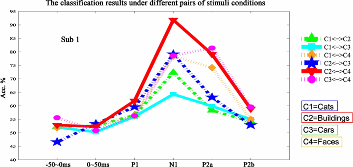
Figure 1. The binary classification results from Subject 1 using different ERP components. The x-axis represents five non-overlapping time intervals corresponding to –50–0 ms, 0–50 ms, P1, N1, P2a and P2b for each subject. The temporal changes of classification accuracies in the curves reveal the separability of features from single ERP components, and depict the temporal distribution of discriminative information for object discrimination. The other subjects have similar binary classification results, which are provided in the supplementary data, available at stacks.iop.org/JNE/9/056013/mmedia.
Download figure:
Standard image3.2. Classification results of combinations of ERP features
We also combined the spatial features from different ERP components and fed the concatenated features to LDA classifiers to explore the effects of feature combination on classification performances.
Figure 2 illustrated the four-category classification results from eight subjects attained after cross-validations using combinations of ERP features. When the feature vectors of multiple ERP components were combined, higher classification accuracies were achieved than those using features from single ERP components. For example, adding the features from P2a to those from N1 (represented by N1+P2a for simplicity) boosted overall four-class classification accuracies by approximately 10–15%, and the combination of P1+N1+P2a also achieved favorable classification performances. The individual four-class classification results of combined ERP features are displayed in table S1, available from stacks.iop.org/JNE/9/056013/mmedia. Similar increases in two-class classification accuracies by combining features from multiple ERP components can be observed in table S2, also available from stacks.iop.org/JNE/9/056013/mmedia.
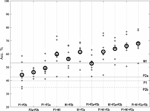
Figure 2. Four-category classification accuracies using combined features from ERP components (P1, N1, P2a and P2b). The classification accuracies from five-fold cross validation procedures are represent by a '+' for each subject and the averaged accuracies across subjects are represented by circles. The averaged classification accuracies across subjects using single ERP features are depicted with four dotted lines for comparisons.
Download figure:
Standard imageIt can also be seen in figure 2 and table S1 (available in the supplementary data), generally speaking, those combined features containing N1 yielded the most favorable classification results. Its rationality may lie in the fact that features from single N1 (N170) component attained better classification results than other single components (table 1 and figure 1) and thus may contain sufficient discriminative information. Another meaningful finding in figure 2 is that N1+P2a get the highest classification results among all the six combinations of two components. To confirm the complementary effects of discriminative information contained in ERP components, we further tested the significance of the differences of classification accuracies between combinations of multiple ERP components. The results of the signrank test in table 2 indicated that the mean classification accuracy of N1+P2a is significantly superior to those classification accuracies of combinations of two ERP components except P1+N1 (p < 0.01). The averaged classification result from eight subjects of N1+P2a is higher than that of P1+N1, but the difference is not significant (p > 0.05). As for the combinations containing three ERP components, P1+N1+P2a obtain the highest accuracy. Table 2 and figure 2 illustrated that P1+N1+P2a attained significantly higher classification results than P1+N1+P2b and P1+P2a+P2b (p < 0.01). However, no significant difference is observed between P1+N1+P2a and N1+P2a+P2b. Table 2 also showed that P+N1+P2a+P2b employing all the single ERP components achieved the best classification performances among all the combinations of features.
Table 2. Results of statistical test (Wilcoxon signrank test) on the improvement of classification accuracies by combining features from multiple ERP components. The values in the table represent the increment of classification accuracies corresponding to the items in the first column after subtracting those corresponding to the items in the first row. For example, the element in the second row and the third column means the accuracy of classifying features from P1+N1 is higher by 6.72% compared to the classification accuracy using N1 features, and the comparison of classification accuracies of P1+N1 and P1+N1+P2a similarly corresponds to the value in the second row and the seventh column.
| P1 | N1 | P2a | P2b | N1+P2a | P1+N1+P2a | |
|---|---|---|---|---|---|---|
| P1+N1 | 20.14%b | 6.72%b | – | – | −1.64% | −6.18%b |
| P1+P2a | 9.63%b | – | 7.43%b | – | −12.15%b | −16.69%b |
| P1+P2b | 4.54%b | – | – | 8.96%b | −17.24%b | −21.78%b |
| P1+N1+P2a | 26.32%b | 12.90%b | 24.12%b | – | 4.54%a | – |
| P1+N1+P2b | 21.99%b | 8.57%b | – | 26.40%b | 0.21% | −4.33%b |
| P1+P2a+P2b | 13.14%b | – | 10.94%b | 17.55%b | −8.64%a | −13.18%b |
| P1+N1+P2a+P2b | 28.19%b | 14.77%b | 25.98%b | 32.60%b | 6.40%a | 1.87%a |
| N1+P2a | – | 8.37%b | 19.58%b | – | – | −4.54%a |
| N1+P2b | – | 3.16%a | – | 20.99%b | −5.21%b | −9.74%b |
| N1+P2a+P2b | – | 10.78%b | 21.99%b | 28.61%b | 2.41%a | −2.13% |
| P2a+P2b (P2) | – | – | 4.30%b | 10.92%b | −15.28%b | −19.81%b |
a p < 0.05. b p < 0.01, eight pairs, and '–' means no comparison applies.
4. Discussion
In this section, we will justify our classification results and discuss the temporal distribution and the complementarity of discriminative information in different ERP components.
4.1. Further discussions about classification results
Our study demonstrated classification accuracies of four-category objects using EEG features from single ERP components and their combinations, suggesting that single-trial EEG responses provide sufficient information to discriminate among faces, cars, cats and buildings.
To justify the classification results, we took note of the classification accuracies using EEG features from pre-onset (−50–0 ms). The classification accuracy of features from this time range should be around the chance rates, because object discrimination processes should not be performed in human brains before visual information presentation. Consistent with this assumption, the six pairs of binary classification results were around 50% for all the eight subjects (figure 1; and figure S1, available from stacks.iop.org/JNE/9/056013/mmedia).
We also randomized the labels of the samples in the training datasets to construct surrogate data (i.e. under the null hypothesis that object categories and EEG features are uncorrelated) for each single ERP component (P1, N1, P2a and P2b). We then trained classifiers using surrogate data and fed the EEG trials for testing to the newly trained classifiers. The six pairs of binary classification results corresponding to all the four ERP components approached 50% (table S3, available from stacks.iop.org/JNE/9/056013/mmedia). This helps confirm that our classifiers indeed utilized category-related information in spatial features from single-trial EEG data, and that the accuracies referring to the baseline (i.e. 50% for binary classification) were reliable.
4.2. Spatial features in averaged and single-trial EEG responses
We will discuss the structure of spatial filters employed by LDA, and compare the spatial features implicitly used by Fisher-LDA with the grand averaging brain topographic maps corresponding to specific ERP components. Figure 3 denotes the averaged ERP time courses from three channels (PO7, PO8 and Cz) and the brain topographic maps of four ERP components/subcomponents from Subject 1. Comparing the brain topographic maps of ERP components from different categories, the between-category spatial difference can be observed in averaged ERP components (represented by µ). For example, we can see from figure 3 that the spatial differences in N1 component were very obvious between faces and non-face categories. In line with previous studies, the spatial features that differ between faces and non-face objects are most obvious at occipital-temporal sites for the N1 (N170) component [31, 32].

Figure 3. The averaged ERP time courses for Subject 1 (butterfly view, elicited by cats, buildings, cars and faces are illustrated in panels A, B, C and D, respectively). The waveforms painted with red, blue and green represent the EEG signals from PO7, PO8 and Cz, respectively. Below the ERP time courses, the brain topographic maps are plotted for four ERP components (P1, N1, P2a and P2b). The trials of EEG responses used for the averaged ERP responses and topographic maps in this figure came from the training dataset of one repetition of cross validation procedures.
Download figure:
Standard imageIn the case of single-trial classification tasks, spatial features in each channel were weighted by the corresponding coefficients of linear classifier w. The vectors of classifiers in six binary classification tasks are depicted in figure 4 by means of a scalp map as introduced in Blankertz et al [29]. It can be seen in figure 4 that projection vector w (also used as spatial filters) of Fisher-LDA indeed have larger weights in the regions with larger between-category differences in the topographic contrast maps in figure 4. Taking the N1 component as an example, scalp maps of LDA coefficients for N1 depicted in the second column of figure 4, especially in the third, fifth and sixth row, resemble the corresponding maps of between-category differences in the fifth column, which indicates that larger weights in the projection vector of classifiers should be given to those channels in the right occipital-temporal areas where between-category differences are prominent.
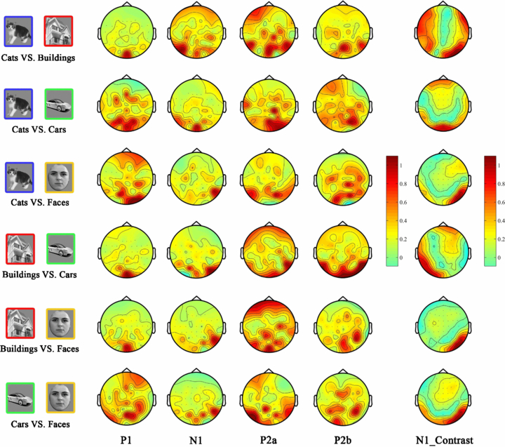
Figure 4. Spatial topographic maps of classifiers and spatial contrast maps of N1 component for Subject 1. The weight maps of the classifiers for EEG features from P1, N1, P2a and P2b components are depicted in the first to the fourth column, respectively. The fifth column shows the spatial contrasts of N1 component between categories. Each contrast map was normalized by dividing by the maximum value among 50 elements of a spatial feature vector. The contrast maps of N1 is indicated here as an example to illustrate the between-category spatial differences.
Download figure:
Standard imageThe comparisons of topographic maps of classifiers and contrast maps of ERP components also show that classifiers do not only focus on obvious features such as the right occipital-temporal areas for N1. They are also sensitive to the between-category differences that are not obvious in grand averaging results. For example, the spatial differences of P1 in the case of cats versus faces in the central sites are barely recognizable in figure 3; however, the classification results indicated that LDA really extracted spatial features from P1 component. A possible explanation is that scalp EEG responses contain both common and discriminatory features, but grand averaging method has the tendency to obscure the trial-by-trial variances in ERP latencies and amplitudes, thus weakening the categorical differences [33]. In contrast, a multivariate statistical tool, such as spatial filter, is able to capture the separable features within multiple channels of single-trial EEG data. In some cases, the discriminatory features (possibly weaker than the common features) revealed by spatial filters are not significant in averaged scalp maps.
Another interesting inconsistency between the contrast maps of the ERP component and the scalp maps of w in figure 4 is that spatial filters are not always smooth. According to Blankertz et al some isolated channels did not provide good discriminability themselves, but they could also have substantial weights in linear classifiers, for they may contribute to the reduction of noise in the informative channels [29].
4.3. Temporal distribution of discriminative information
Single-trial classification accuracy, in a sense, serves as an objective index to evaluate the discriminative information in EEG features. The fluctuations of classification accuracies of different ERP features are depicted in figure 1; and figure S1 (available from stacks.iop.org/JNE/9/056013/mmedia). The sequential ERP components could reflect different processing stages of visual information—including low-level encoding mechanisms and high-level behavioral processes [34, 35]. The results of classifying these features from segmented ERP components showed that the different discriminative information contained in each ERP component induced the temporal changes of classification accuracies. The results demonstrated that the accuracy of binary identification rates start to exceed 50% from the P1 component, indicating that P1 contains discriminative information while those components earlier than P1 may contain very little, if any, discriminative information. It is then worth pointing out that our classification results may be driven by the low-level features of the presented objects. The classification performances of P1 and N1 may suggest that the majority of discriminative information could be derived from the early structural encoding process.
Classification results for the P2a and P2b in table 1 indicated that features from the late ERP component also provide discriminative information for object discrimination. However, the classification accuracies using EEG features from P2a or P2b were not as high as N1, because P2a/P2b occurs at a late stage when little low-level physical features of the visual stimuli are being processed. Another reason lies in the fact that late ERP component/subcomponent is more susceptible to individual variances and behavioral noise.
It is worth noting that spatial features used by classifiers change over time. Figure 4 demonstrated the weight maps of classifiers for N1 have stronger activations in the occipital region, while weights of P2a and P2b classifiers were scattering across the whole scalp. Weight maps of classifiers for ERP components revealed varying spatial differences in scalp electrophysiological responses over time. Further discussions in the following section will demonstrate that changes of spatial features across components could provide temporal information favorable for classification. Another question is whether the constant spatial feature extracted from a time interval or an ERP component is too stable to reflect the changes of spatial differences over time. According to Tzovara et al brain states remain stable for periods of several tens of milliseconds, independently of changes in response strength [36]. Thus, the way in which we averaged each ERP segment along time is reasonable to capture the stable spatial features in each ERP component while maintaining the temporal characteristics of changes of spatial features among different ERP components.
4.4. Combining ERP features for discriminating objects
Classification results using combinations of the ERP features confirmed the complementarity of discriminative information from different ERP components. These characteristics of ERP features suggest that it is necessary to integrate and make full use of the discriminative information contained in multiple ERP components in an appropriate way to improve object discrimination performances.
We can see in table 2 that the concatenated EEG features yielded significantly higher classification accuracies. The improved classification performances by combining ERP features, such as N1+P2a, may be ascribed to the better complementarity between features from N1 and P2a. Furthermore, if only classification accuracies were considered, the combination of P1+N1+P2a generally yielded better performances than N1+P2a, suggesting that P1 could still provide complementary discriminative information to N1+P2a. However, P1+N1+P2a consumed larger data volume but only achieved higher accuracies than N1+P2a by no more than 5% on most subjects (figure 2).
To further improve classification performance of multi-class objects using single-trial EEG, machine learning and pattern recognition methods should play more important roles. For example, a separate feature extraction could be performed prior to EEG classification to mine the discriminative information. To utilize temporal and spatial features in EEG simultaneously, one approach is to design a sequence of spatial filters, each for one ERP component, and then to combine those spatially filtered features [17]. In the present study, LDA was used to classify EEG features from single ERP component. We did not design an explicit feature extraction step, and we used the average of EEG across time samples in time intervals as EEG features (i.e. spatial features because of containing only one sample in time [29]). Our study showed that temporally averaged spatial features of ERP components (P1, N1, P2a and P2b) indeed contain object category-related information for classification. When the pure spatial features were concatenated to form new long feature vectors (spatial-temporal features), the LDA classifier then utilized the temporal information in the sequential ERP spatial features and also utilized the implicit complementary information in different ERP components.
4.5. Classification results using general features across subjects
We have described the classification results using subject-specific features, i.e. we trained and tested a specific classifier using the features from one subject. In order to compare the general features and individual features, we employed a leave-one-subject-out cross-validation approach to study the classification of general features.
Each time we pooled all the trials from seven subjects for training and thus there were a total of 350×4×7 trials from four categories (350 trials for each category for each subject) in the training dataset. And all the 1440 trials (350×4×1) from the other subject were used as the testing dataset. We extracted ERP features from training data, used them to train the Fisher-LDA classifier, and then validated it using testing dataset. The cross-validation results were shown in table S4 (available from stacks.iop.org/JNE/9/056013/mmedia). The results suggested that the distribution tendencies of discriminative information among P1, N1, P2a and Pb2 still hold across subjects and further confirmed that discriminative EEG information indeed came from the common brain activities across subjects during object discrimination tasks. Here, all the eight subjects shared the same time widow length for ERP components. The ranges of ERP components were listed in table S5 (available from stacks.iop.org/JNE/9/056013/mmedia).
4.6. Impacts of category number on object discrimination
Compared to previous classification studies, we achieved similar classification accuracies in binary classification tasks [16–18]. We further presented four-class classification results in table 1 to investigate the impact of including more than two categories in the discrimination task. By including four categories, the classification results decreased by 15–20% compared to binary classification results but are still statistically significantly higher than chance, suggesting the possibility of discrimination of multi-category objects. In our study, when combining EEG features from different ERP components, the best classification performances can be maintained as high as around 65–70% for most subjects.
It is still worth noting that the classification results can be affected by which categories of objects we want to discriminate. For example, we have shown that faces can be more easily discriminated from non-face objects and thus attain higher classification accuracies. Hence, the four categories of common objects used in our study, faces, cars, cats and houses, can be discriminated effectively using single-trial EEG, which may contribute to the object discrimination studies.
Acknowledgments
We thank Dr Zhihao Li in Biomedical Imaging Technology Center of Emory University/Georgia Institute of Technology for helping us in collecting the EEG data used in this study. This work is supported by the National High-tech R&D Program (863 Program) under grant number 2012AA011600 and the Fundamental Research Funds for the Central Universities. This work is also supported by the Major Research Plan of the National Natural Science Foundation of China (NSFC) Key Program 60931003.