

Abstract
We present the design, fabrication, modeling and feedback control of an earthworm-inspired soft robot capable of bidirectional locomotion on both horizontal and inclined flat platforms. In this approach, the locomotion patterns are controlled by actively varying the coefficients of friction between the contacting surfaces of the robot and the supporting platform, thus emulating the limbless locomotion of earthworms at a conceptual level. Earthworms are characterized by segmented body structures, known as metameres, composed of longitudinal and circular muscles which during locomotion are contracted and relaxed periodically in order to generate a peristaltic wave that propagates backwards with respect to the worm's traveling direction; simultaneously, microscopic bristle-like structures (setae) on each metamere coordinately protrude or retract to provide varying traction with the ground, thus enabling the worm to burrow or crawl. The proposed soft robot replicates the muscle functionalities and setae mechanisms of earthworms employing pneumatically-driven actuators and 3D-printed casings. Using the notion of controllable subspace, we show that friction plays an indispensable role in the generation and control of locomotion in robots of this type. Based on this analysis, we introduce a simulation-based method for synthesizing and implementing feedback control schemes that enable the robot to generate forward and backward locomotion. From the set of feasible control strategies studied in simulation, we adopt a friction-modulation-based feedback control algorithm which is implementable in real time and compatible with the hardware limitations of the robotic system. Through experiments, the robot is demonstrated to be capable of bidirectional crawling on surfaces with different textures and inclinations.
Export citation and abstract BibTeX RIS
1. Introduction
Animal locomotion has long been a source of inspiration for robotic research. In particular, limbless locomotion has attracted significant attention as it is regarded as one of the most effective methods of traveling on unstructured terrains [1–3]. Among the most studied limbless forms of locomotion are the peristalsis-based gaits obseved in earthworms (Lumbricidae). Within the earthworm family, some species can travel both under and above ground; for example, nightcrawlers (Lumbricus terrestris) typically remain underground during the day but travel above ground at night [4, 5]. As a result of these behaviors, nightcrawlers evolved burrowing and crawling as two distinct methods of travel which allow them to maneuver and navigate through labyrinthine underground burrows and complex terrains, respectively. In both cases, the exhibited gaits are peristalsis-based, produced by the coordinated and successive contraction and relaxation of the longitudinal and circular muscles in the nightcrawlers' metameres [6]. These repeating patterns can be thought of as retrograde waves that propagate along the axial axes of the animals in the opposite direction of travel to produce either forward or backward thrust. The generated thrust is converted to locomotion through traction with the ground, which is modulated by the action of microscopic bristle-like structures known as setae [4, 7].
Versatility, robustness and spatial efficiency make the earthworms' peristaltic gait a very attractive natural model for the development of robotic locomotion. Consistently, numerous research projects have focused on creating robots that can replicate earthworms' peristalsis-based locomotion, adopting a variety of different actuation technologies, including electric motors [8–10], magnetic fluids [11] and shape-memory-alloys (SMAs) [12–14]. Also, systems that integrate origami-inspired folding structures with embedded actuators have been demonstrated to be suitable for creating robotic mechanisms capable of producing large bidirectional deformations which mimic the motions of earthworms' circular and longitudinal muscles [15, 16]. Additionally, recent innovations in design, fabrication and utilization of soft and liquid materials have enabled the development of biologically-inspired soft actuators, soft sensors and flexible electronics [17–19]. In this work, by integrating these technologies, we introduce a new modular soft robot whose conceptual design is inspired by the morphologies and functionalities of earthworms' muscle structures and traction mechanisms based on the use of setae.
As shown in figure 1, the proposed robot is composed of one central axial pneumatic actuator, which produces forward and backward thrust; two extremal (back and front) pneumatic actuators encapsulated by 3D-printed casings, employed to control traction; and three flexible pipe lines employed to inject and extract air into and out from the actuators, respectively. In this design, to produce peristalsis-based crawling motions, the axial longitudinal actuator extends and contracts to generate deformations and forces analogous to those produced by earthworms' longitudinal muscles; while the two encapsulated pneumatic extremal actuators serve functions analogous to those of earthworms' circular muscles and setae, i.e. modulate the frictional forces needed to alternately anchor the robot's extremes to the ground during crawling.
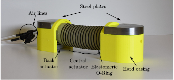
Figure 1. The earthworm-inspired soft robot capable of bidirectional locomotion presented in this work. The system is composed of two 3D-printed hard casings, one central actuator constrained by elastomeric o-rings, two extremal (front and back) actuators, two machined steel plates and off-the-shelf pneumatic components.
Download figure:
Standard image High-resolution imageIn the technical literature, it has been common to categorize segmented robots composed of three or fewer actuation modules as inchworm-inspired [20], regardless of the underlying mechanisms of locomotion; there are several fundamental features, however, that clearly distinguish the locomotion modes of earthworms, employed as inspiration in this work, from those of inchworms (caterpillars of geometrid moths). For example, it has been observed that the crawling of Manduca sexta caterpillars is generated through a series of steps that resemble the walking of animals with rigid skeletons and that these larvae use longitudinal body shortening to power their movements rather than the constriction and elongation performed by worms [21]. Additionally, during inching, caterpillars use strong gripping forces supplied by their true legs and prolegs to sustain their bodies while curving in omega ( ) shapes, which is a behavior unique to inchworms [22]. Thus, in an abstract sense, the robot proposed here is better described as a two-metamere artificial earthworm rather than as an inchworm, despite its three-module configuration.
Almost all forms of animal and robot terrestrial locomotion rely on friction-induced traction [23, 24] and frictional anisotropy is the underlying mechanism behind a significant number of animal gaits, including serpentine crawling [25]. Specifically, snakes use the geometric anisotropic patterns of their skins to induce frictional forces with magnitudes that depend on the direction of friction, thus causing net body displacements along the direction with the smallest opposing frictional force when slithering. Drawing inspiration from these nature's examples, researchers have developed a class of robots that exploit frictional anisotropy to travel [15, 26–28]; these systems, however, use friction as a passive mechanism as frictional forces are not actively modulated to control locomotion. Moreover, anisotropic-friction-induced locomotion is inherently unidirectional, which limits animals with anisotropic skins and their corresponding bioinspired robots to travel along directions in a constrained set. Thus, from a pure engineering perspective, it is clear that friction-controlled bidirectional locomotion has numerous advantages for the creation of agile soft robots, as the direction of motion can be changed from forward to backward almost instantaneously without the need for a body reorientation.
In an attempt to achieve bidirectional locomotion, the work in [29] introduces a soft robot that travels with a gait similar to those exhibited by caterpillars, actuated by a motor-tendon mechanism. In that design, the bidirectional rotation of an electric motor is employed to switch between two regions of contact of the robot with the ground (made of different materials), thereby manipulating the distribution and magnitudes of the friction forces acting on the robot's body in order to generate either forward or backward motion. That mechanism is ingenious and was demonstrated to be effective and robust; however, it is not clear how the same design principles can be applied to the development of controllable complex modular configurations. In contrast, the crawling motion of earthworms can be readily modularized as these animals coordinately anchor some of their metameres to the ground by protruding setae that increase traction while other body segments undergo deformations (contractions or extensions); this mechanism also enables earthworms to travel bidirectionally [7].
The robot presented in this paper is modular and capable of bidirectional crawling using a simple, yet reliable, controlled frictional-force-based set of actions executed by the extremal encapsulated actuators shown in figure 1. Specifically, the extremal actuators actively vary the frictional forces acting on the front and back of the robot by switching the surfaces of contact with the ground, which are made of different materials with distinct friction coefficients. In this scheme, when an extremal actuator is inflated, its rubber surface touches the ground surface (a contact with high friction); and when an extremal actuator is deflated, its rubber surface does not touch the ground and the weight of this extreme of the robot is supported by the corresponding hard casing (a contact with low friction). As experimentally demonstrated in section 6, the proposed robot is not only capable of locomoting forward and backward on horizontal surfaces but also on inclined planes.
To generate feasible locomotion patterns for the robot, we propose a control strategy based on a reduced-complexity description of the system's dynamics. This approach allows us to study the robot's controllability and its relationship with friction, a complex nonlinearly-generated type of force that has been modeled using numerous different methods [31–33]. Here, we employ a friction model that includes the stick-slip effect, a phenomenon that must be considered in the dynamical descriptions of most ground-traveling robots and has been extensively studied in the technical literature. For example, in [34–36], stick-slip is discussed and included in the modeling of generic worm-like robots, while [37] explores its effects when a worm-inspired robot moves inside compliant structures. Also [38] and [39] show that vibration-induced stick-slip can be directly exploited to generate locomotion.
By treating the axial force generated by the central actuator as well as the nonlinearly-generated time-varying frictional forces produced by the extremal actuators as system inputs, the dynamics of the proposed robot (figure 1) can be described with a linear time-invariant (LTI) state-space representation. This model enables us to analyze the controllability of the system from a simplified LTI perspective and determine that friction is indispensable for this robot, and other mechanisms of this type, to generate locomotion. Namely, in the absence of friction, the controllable subspace of the system contains only states that characterize a static center of mass with respect to any inertial frame defined to describe the dynamics the system. Furthermore, it can be shown that if the axial force generated by the central actuator and the forces acting on the extremes of the robot could be chosen unrestrictedly, the system would become fully controllable. This finding, despite being based on physically unattainable assumptions, indicates that there exists an infinite number of theoretically feasible traveling modes. Thus, it can be deduced that biologically-inspired locomotion modes represent only a small set of what can possibly be achieved with this framework.
The work in [30] introduced an earthworm-inspired burrowing soft robot (figure 2) designed to locomote inside pipes for inspection and maintenance applications. The functionality of that robot is confined to the interior of tubes with diameters in a limited predefined range. Thus, the work presented in this paper expands and complements the capabilities of the system in [30], and it is intended to serve as a platform for creating soft robots capable of both crawling and burrowing. Furthermore, the real-time algorithm developed for locomotion control can be extended and applied to other types of modular robotic systems to achieve bidirectional locomotion on steep inclines or even vertical surfaces. The rest of the paper is organized as follows. Section 2 discusses earthworm locomotion as inspiration for soft robotic development, section 3 describes the design and methods employed in the fabrication of the proposed robot, section 4 presents the dynamical description of the system and its controllability analysis, and section 5 shows locomotion simulation results. Experimental results are presented and discussed in section 6. Lastly, section 7 draws some conclusions and states directions for future research.
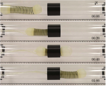
Figure 2. Photographic sequence composed of movie stills showing the horizontal burrowing locomotion of the earthworm-inspired soft robot introduced in [30]. This robot, in contrast with that presented in this article (figure 1), can only travel inside pipes with diameters in a predefined range because its locomotion mode and functionalities are highly specialized to tube-like structured paths.
Download figure:
Standard image High-resolution image2. Earthworm-inspired locomotion
Earthworms belong to the phylum Annelida, characterized by segmented bodies composed of metameres [4]. During locomotion, each body segment is actively reshaped by contractions and relaxations of its longitudinal and circular muscles. Specifically, as illustrated in figure 3(a), metameres expand radially (shortening longitudinally) as their longitudinal muscles contract, and elongate (shrinking radially) as their circular muscles contract [6]. These active isochoric body reconfigurations are possible because metameres are composed of deformable anatomical structures referred to as hydrostatic skeletons. In this layout, body segments are separated from each other by impermeable septa and their internal cavities (coeloms) are filled with incompressible coelomic fluid [6]. Thus, to induce locomotion, each metamere alternately cycles through a constant-volume muscle-actuated longitudinal elongation and a radial expansion, generating a wavelike motion along the body, as depicted in figure 3(b). Note that this peristaltic wave propagates in the opposite direction of locomotion [40]. To model and replicate peristalsis-based locomotion for worm-inspired robots, researchers have explored a wide variety of methods, including finite-state machines [41]; genetic algorithms [34]; actuation phase coordination [42]; and adaptive controllers, which are employed to track prescribed reference lengths between segments [43].
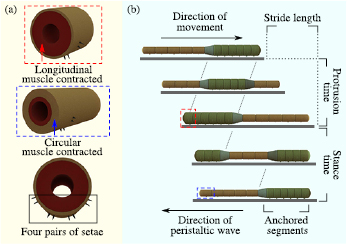
Figure 3. (a) Illustration of a nightcrawler's metamere. A metamere expands radially when its longitudinal muscles contract (circular muscles relax) and expands longitudinally when its circular muscles contract (longitudinal muscles relax). In this depiction, the four pairs of setae on the ventral and lateral surface of the metamere protrude and retract jointly with the contraction and relaxation of the longitudinal muscles to provide variable traction during locomotion. (b) Peristalsis-based crawling. Following the convention in [4], we define a stride as a complete cycle of peristalsis and describe the crawling kinematics as a function of four variables: stride length, protrusion time, stance time and stride period.
Download figure:
Standard image High-resolution imageAll Oligochaetas, which are a subclass of the phylum Annelida that includes earthworms, bear retractable setae in their metameres [6]. Some species of earthworm are both geophagous (earth-eaters) and surface-feeders, which is the case for nightcrawlers [4]. For nightcrawlers, setae perform the critical function of providing adequate traction so that peristaltic body waves can be transformed into either forward or backward locomotion, especially when crawling above ground. Consistently, nightcrawlers have evolved setae only on the ventral and lateral surfaces of their metameres, as depicted in figure 3(a), while purely geophagous earthworms have setae arranged in a ring around each metamere [7, 44]. When a metamere undergoes radial expansion (longitudinal muscle contraction), its setae protrude to anchor that section of the body to the substratum in order to prevent slipping while adjacent metameres initiate their own reconfigurations as shown in figure 3(b). Then, once the metamere's circular muscles start to contract, the longitudinal muscles subsequently relax, thus pulling the setae off from the ground to allow the metamere to slide.
To devise a gait for the proposed robot in figure 1, we draw inspiration from the nightcrawlers' crawling mode; which is modeled by the sequence illustrated in figure 3(b) according to data from the biological literature [4]. Consistently, we define a stride as one cycle of peristalsis; the stride length as the total distance covered during one stride; the protrusion time as the time span in a cycle during which the nightcrawler's head moves forward to cover the stride length; the stance time as the time span in a cycle during which the nightcrawler's head remains anchored to the ground while the rest of its body moves forward and returns to its initial geometric configuration; and the stride period as the time that it takes to complete one entire stride, which is equivalent to the sum of the protrusion and stance times. Despite the fact that nightcrawlers have nume-rous segments with staggered stride periods, these variables are the most adequate to describe the considerably simpler kinematics of the robot in figure 1, and to define feasible locomotion patterns, because this system was conceived and can be modeled as an artificial two-metamere earthworm. During backward locomotion, the protrusion and stance times (and other kinematic variables) are defined with respect to the tail instead of the head.
3. Design and fabrication
The robotic design in figure 1 is an extension of the work in [30], which presents a soft robot that employs a burrowing-inspired gait to locomote inside pipes (see figure 2). In this section, we present the design and fabrication tools developed for creating the proposed new robot (see figure 4), which is capable of locomoting bidirectionally on horizontal and inclined flat surfaces, employing a peristalsis-based friction-controlled crawling mode inspired by that performed by earthworms. In this case, the problems of robotic design, fabrication, locomotion planning and control are strongly coupled, as the the proposed bioinspired friction-based locomotion scheme relies not only on a digital controller but also on control functions preprogrammed in the physical components of the robot. A key innovation in this approach is the apparatus that enables the active variation of the friction coefficients associated with the sliding of the extremal actuators, which can switch their surfaces of contact with the ground in order to modulate friction forces. This technique is used to replicate the combined active–passive mechanisms employed by earthworms for locomotion and control discussed in section 2; consistently, as seen in figure 1, the robot is powered by one pneumatically-driven central longitudinal actuator while the pneumatically-driven extremal actuators are required for control.

Figure 4. (a) Fabrication of the extremal actuators. In step 1, liquid silicone is poured into a 3D-printed mold; then, the lower half of a symmetrical double-cylindrical core is submerged in the silicone. The silicone within the mold is then cured at  for
for  . In step 2, the cured silicone is released before liquid silicone is added to cast the other half of the shell (steps 3 and 4). Step 5 shows the complete shell structure after being peeled off from the 3D-printed core. In step 6, o-rings are fitted onto the shell's imprinted grooves, and a layer composed of silicone and a fiberglass net is employed to seal one end of the shell. Step 7 shows a extremal actuator once the fabrication process is completed. (b) and (c) Fabrication of the central actuator and connecting modules. These procedures are identical to those employed in (a) with the exception that the connecting modules do not require an additional reinforcing layer and o-rings. Additionally, an orifice is perforated from the bottom of both connecting modules to allow the flow of air into both of extremal actuators. (d) Final assembly. In step 1, the two extremal actuators, the central actuator, two connecting modules and three air-supplying lines are integrated together. In step 2, a pair of 3D-printed casings are fixed over the connecting modules of both extremal actuators. Step 3 depicts the cross-sectional view of the robot in two states: all the actuators inflated and all the actuators deflated. Finally, step 4 shows the robot after the fabrication process of the entire robot is completed.
Download figure:
Standard image High-resolution imageThe central and extremal actuators emulate the functionalities of an earthworm's longitudinal and circular muscles, respectively. These three actuators are fed through independent air lines, and were designed and built to expand and contract axially according to empirically-estimated functions of their internal pressures. The radial expansions are constrained with black butadiene rubber elastomeric o-rings as seen in figure 1. As discussed in section 2, during locomotion, nightcrawlers adjust traction with the ground by combining the effects produced by the protraction–retraction of setae and deformations of their hydrostatic skeletons. Similarly, the proposed robot adjusts the frictional forces acting on the extremal actuators by changing the surfaces of contact with the ground; therefore, also changing the associated coefficients of friction when the materials of these surfaces are different. According to the literature on friction [45], the coefficients of kinetic friction can vary widely depending on the types of surfaces in contact; for example, the coefficient for Teflon on steel is approximately 0.04 while the coefficient for rubber on concrete is approximately 0.8, which indicates that there is a wide range of possibilities for the design and implementation of locomotion strategies.
The design of the extremal actuators is such that their inflatable soft structures are made of silicone rubber whose contact with any other surface is characterized by a friction coefficient with a high value while the contacts of the enclosing 3D-printed casings with any other surface are characterized by friction coefficients with low values. Thus, as shown in the bottom illustration of figure 4, since the inflatable extremal actuators are fixed to the ceilings of their corresponding casings, their rubber surfaces do not touch the ground when deflated and the robot's body is supported by the hard casings. On the other hand, the rubber surfaces of these actuators make contact with the ground when their inflatable structures are inflated, thus inducing high values of friction. In this scheme, the switching between high and low friction states, and vice versa, is accomplished by simply inflating and deflating the friction actuators, and vice versa.
Unlike existing robots which employ frictional anisotropy [15, 26–28], for which the direction of friction is determined by the morphology and skin patterns of the structures in contact with the ground, the proposed robotic design was conceived to generate controllable isotropic frictional forces. This method for active friction control has the potential to enable earthworm-like crawling in any conceivable direction in a plane by either increasing the number of modules or/and the number of friction actuators. In this case, given the linear two-metamere axially-powered configuration of the robot, it can crawl and be controlled bidirectionally (forward and backward). Note that even though the functionalities of the extremal friction actuators are inspired by those of earthworms muscles and setae, the underlying working principles are fundamentally different. For example, earthworms protract setae to increase traction because their skins are smooth and low-friction while the robot employs the direct contact of its rubber skin with the ground to increase friction. In addition, natural muscles contract actively and elongate passively while the pneumatic actuators of the robot elongate actively and contract passively.
The methods and construction sequences employed to fabricate the soft robot are depicted in figure 4. As shown in figures 4(a)–(c), the extremal actuators, the central actuator and connecting modules are fabricated by casting liquid silicone (Ecoflex® 00-50, Smooth-On) in 3D-printed acrylonitrile butadiene styrene (ABS) molds. The yellow casings are also 3D-printed using the same ABS material employed to create the casting molds. The final assembly of the robot, in which all the individual parts are put together, is illustrated in figure 4(d). At this fabrication stage, all the interfaces are airtight sealed using liquid silicone and extendable coiled air supply lines are inserted into the central and front actuators. Note that the coil shape of the internal air lines is the key design feature that allows the pneumatic actuators to freely expand and contract.
The inflatable structures of the central actuator and both extremal actuators are 35 mm in diameter and have homogeneous walls with a thickness of either 2.5 mm or 3 mm depending on the location in the soft structure. The central actuator has a length of 83 mm and weighs 51 g including the o-rings and air supply lines; each extremal actuator combined with a connecting module has a total length of 26 mm along its axial direction and weighs 19 g; and each 3D-printed casing weighs 18 g. These dimensions were initially selected to replicate those of the robotic design in [30] and then modified to fit the required off-the-shelf pneumatic components. Finally, as can be observed in figure 1, after the final assembling in figure 4(d) is completed, 130 g steel plates are fixed to the tops of the yellow casings in order to increase the maximum friction forces attainable with the proposed actuation scheme.
4. Dynamic modeling and controllability
In this section, employing a reduced-complexity dynamic model and linear systems theory, we develop the analytical tools necessary to study the motion and controllability properties of the robot described in section 3. From an abstract perspective, the dynamics of the proposed robot can described by a double-mass-spring-damper model [43, 46, 47] excited by active actuation forces and time-varying friction forces, as illustrated in figure 5. Accordingly, the extremal actuators are modeled as two blocks, with masses m1 and m2, capable of varying their coefficients of friction with the supporting ground surface in real time in order to modulate the values (signed magnitudes) of the frictional forces, f 1 and f 2 in figure 5. Similarly, given its function and the elastic nature of its soft structure, the central axial actuator is modeled as a system composed of a massless elastic spring with stiffness constant k, a dissipative element with constant c and two pneumatically-generated actuation forces with opposite directions and identical magnitudes  (see figure 5). In this model, the radial expansion of the actuator is considered to be completely negligible; therefore,
  can be estimated as

where  and
and  are the instantaneous internal air pressure and constant cross-sectional area of the actuator, respectively. Note that in agreement with the findings in [30], we assume a constant value of k, which is sufficiently accurate for the purposes of controllability analysis and controller synthesis; the true stiffness, however, is nonlinear, time-varying and most likely depends on the internal air pressure of the actuator.
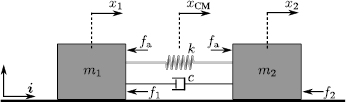
Figure 5. Reduced-complexity double-mass-spring-damper model of the robot in figure 1. The associated mathematical description of this model is employed to study the controllability of the robot in the absence and presence of forces f 1 and f 2. To model friction, the values of f 1 and f 2 are considered to be positive when the associated force vectors act in the same direction as that of  ; consistently, the values of f 1 and f 2 are considered to be negative when the force vectors act in the opposite direction as that of
  .
.
Download figure:
Standard image High-resolution imageTo study the controllability of the system, we first consider the frictionless case in which the sole input to the system is the force magnitude  . Consistent with figure 5, we define x1 and x2 as the position variations of m1 and m2 with respect to the inertial frame of reference; and correspondingly, the associated speeds as
  and
and  . Thus, for the purpose of analysis, the system is described with the single-input–multiple-output (SIMO) state-space realization
where
and  .
.
In this case, for any conceivable choice of parameters m1 > 0, m2 > 0 and k > 0, the controllability matrix ![$ \newcommand{\e}{{\rm e}} \mathcal{C}_{0} = \left[\begin{array}{@{}cccc@{}} B_0 & AB_0 & A^2B_0 & A^3B_0 \end{array} \right]$](https://content.cld.iop.org/journals/1748-3190/14/3/036004/revision2/bbaae7bbieqn014.gif) has rank 2; therefore, the system is not controllable. This implies that there exists a set of states that cannot be reached from any given initial state by employing an input signal [48]. To determine if the uncontrollability of the system prevents locomotion, we further investigate the controllable subspace associated with the pair
has rank 2; therefore, the system is not controllable. This implies that there exists a set of states that cannot be reached from any given initial state by employing an input signal [48]. To determine if the uncontrollability of the system prevents locomotion, we further investigate the controllable subspace associated with the pair  , defined as
  . As explained in [49], it can be shown that
  is also the set of states that can be reached from the initial condition
  by employing an input signal,
  . In particular, it follows that
  , in which
Therefore, every state in  can be written as
  for some
  ,
,  , which implies that all the positions of m1 and m2 that can be reached from
  have the form
  . Thus, we conclude that for an initial state
  , the position variation of the system's center of mass
  with respect to the inertial frame will remain unchanged regardless of what input signal
  is employed to excite the system, because
for all  . Hence, in the absence of frictional forces, locomotion is impossible for robots of the type in figure 5. This finding is consistent with basic physical intuition (the sum of forces acting on the system is zero) and biological observations [40, 50].
When friction is included in the model of the robot, the sliding blocks are alternately subjected to either static or kinetic friction, depending on their relative motions with respect to the surface; a rapid variation between these two types of friction is the phenomenon commonly referred to as the stick-slip effect. Here, we model the friction force associated with the sliding block i, f i, according to the method in [32], as
where,  is the kinetic friction affecting the mass;
  is the net force jointly exerted by the spring, damper and actuator on the block;
  , with
  , defines a narrow band of speed near zero, outside which the mass slips and is affected by the kinetic friction
  ; and
; and  is the maximum value that the magnitude of the static friction force can take. The kinetic friction associated with each block is modeled as

for  , where
  is the corresponding kinetic friction coefficient; g is the acceleration of gravity constant; and
  is the angle of the surface that supports the block with respect to the horizontal. Similarly, the critical value
  is estimated as

for  , where
  is the corresponding static friction coefficient and
  is the magnitude of the static normal force exerted by the mass mi on the supporting surface. Also, from Newton's laws, it immediately follows that the signed (positive or negative) magnitude of the net force is simply

for  . Thus, according to this idealization, when the signed speed of the block i lies within the range
  and the frictional force equals the sum of all the other external forces acting on the mass mi,
  , the block is considered to be sticking. When the magnitude of
  exceeds that of
  (i.e, the static frictional force is too small to counteract all the other external forces), slipping occurs and the friction acting on the block i is
  according to (6).
Following the model in (5), if the masses of the blocks remain constant, f 1 and f 2 can only be modulated by varying the associated coefficients of friction. Using linear-system-theory-based analyses only, it is not possible to determine whether the system would become fully controllable when the inputs are chosen to be  . However, to study the importance of friction in the control of locomotion, we analyze the case in which the inputs
  are assumed to be unconstrained and arbitrarily choosable. Under this assumption, the system can be described using the multi-input–multi-output (MIMO) state-space representation
  , where the new input state matrix and input signal are given by
The controllability matrix associated with the augmented state-space realization  ,
, ![$ \newcommand{\e}{{\rm e}} \mathcal{C}_1 = \left[\begin{array}{@{}cccc@{}} B_1 & AB_1 & A^2B_1 & A^3B_1 \end{array} \right]$](https://content.cld.iop.org/journals/1748-3190/14/3/036004/revision2/bbaae7bbieqn054.gif) , has rank 4; therefore, the controllable subspace
, has rank 4; therefore, the controllable subspace  spans
spans  , i.e. the system defined by (9) is fully controllable. This analysis shows that if the input u1 could be selected without restriction, any desired final state (and any position of the system's center of mass) could be reached in a finite amount of time. In the case of the robot in figure 5, however, u1 is strongly constrained by the limitations of the actuators and the time-varying nonlinear nature of the frictional forces acting on the sliding blocks. Despite these restrictions, controlled locomotion is achievable by varying the coefficients of friction in (5), which is demonstrated through the numerical simulations and experiments discussed in the next sections.
5. Locomotion simulation
In this section, through numerical simulations, we demonstrate that the proposed robotic system can generate locomotion using feedforward-controlled time-varying friction. In this case, a set of feasible control inputs is selected via an exhaustive search followed by an iterative numerical process. According to (6) and (7), the values of the frictional forces f i are functions of the normal forces exerted by the blocks on the supporting surface and the corresponding coefficients of friction (static or kinetic). As discussed in section 3, the robot in figure 1 regulates the friction forces f 1 and f 2 by varying the associated friction coefficients in real time while the normal forces remain constant. Specifically, the inflatable structures of the extremal actuators, made of silicone rubber, induce a high friction coefficient,  or
or  , when in contact with the supporting surface while the 3D-printed casings induce a low friction coefficient,
  or
or  , when in contact with the same surface.
To estimate the achievable range of values for the friction coefficients induced by the silicone rubber and ABS-printed casings when in contact with a supporting surface, we place the robot on an inclined plane covered with a test material; then, we slowly increase the angle of inclination until the robot starts to slip and eventually slides down. To explain the details of the method, as an example, here we describe the tests and estimation process corresponding to a supporting surface made of high-density polyethylene (HDPE). This procedure was repeated twice for each pair of surfaces in contact, i.e. silicone rubber in contact with the ground when the inflatable structures of the extremal actuators are inflated and ABS material in contact with the ground when the inflatable structures of the extremal actuators are deflated. The specifics of the experimental method employed to estimate the friction coefficients are as follows. In static equilibrium, the mechanics of the system can be described by

for  , where
  is the tangential component of the weight mig, which equals the static frictional force acting on the block i, f i. At the critical equilibrium angle
  (right before slipping occurs), (10) becomes

Thus, the static coefficient of friction can be estimated as
Experimental data obtained employing the complete robotic prototype in figure 1 indicate that the critical angle  for the contact of silicone rubber with the HDPE surface is approximately
  and for the contact of ABS material with the HDPE surface is approximately
  . These angle values translate to static coefficients of friction of approximately
  and
and  , respectively. In these experiments, however, the tangential weight components of the robot's steel plates (shown in figure 1) induce bending and twisting on the soft structures, thus disrupting the contacts between the extremal actuators and the inclined supporting surface. If the steel plates are removed, the shear forces exerted on the actuators can be drastically reduced, enabling the robot to maintain a firm contact with the supporting HDPE board at much steeper slopes. In experiments, the robot remains stationary on a HDPE surface with a slope as large as
  with respect to the horizontal before starting to slip. Correspondingly, the static friction coefficient is estimated to be as large as
  , which is likely an estimation closer to the true value. Further details about the experiment-based estimation process can be found in the supplementary movie BBS1.mp4 (stacks.iop.org/BB/14/036004/mmedia).
The purpose of performing an experiment-based estimation of the friction coefficients is to obtain a guideline in the selection of the parameters employed in the numerical simulations of the robot's locomotion, for which we have to define static and kinetic coefficients for the two types of contacts employed by the extremal actuators. Since here we are not trying to exactly replicate experimental data through simulations but to study the proposed method of locomotion, consistent estimates with values in the same range as those in the literature are sufficient for numerical implementation. Following this principle, despite expected experimental inaccuracies, we also estimate the kinematic coefficients of friction empirically, informed by the fact that their values should be smaller than the corresponding parameters for the static case [51]. Specifically, we measure the forces required to initiate and maintain the sliding motion of the robot using a spring scale, for the two types of contacts experienced by the extremal actuators (i.e. silicone rubber sliding on HDPE and ABS material sliding on HDPE). The obtained empirical results indicate that regardless of the contact surfaces involved in the experiments, the estimated value for the kinetic friction coefficient in every case is approximately  the estimated value for the corresponding static friction coefficient. Consistently, in the implementation of the simulations, we employ
 and
and 
 . Additional experiments performed to identify the dynamic characteristics of the inflation-deflation-based friction switching mechanism employed by the extremal actuators indicate that the transitions between
  (or
(or  ) and
) and  (or
(or  ), for
  , can be completed within
  . This finding allows us to model the cyclic switching between high and low friction coefficients assuming a quasi square-wave signal.
The numerical simulations of the system's dynamics during locomotion are implemented according to the block diagram in figure 6(a). Here,  is the discrete-time input-output dynamic description of the robot with input
 ![$u_1[n] = \left[~ f_{{\rm a}}[n]~f_1[n]~f_2[n] ~\right]^T$](https://content.cld.iop.org/journals/1748-3190/14/3/036004/revision2/bbaae7bbieqn083.gif) and output
and output ![$x[n]= \left[~ x_1[n]~x_2[n]~v_1[n]~v_2[n] ~\right]^T$](https://content.cld.iop.org/journals/1748-3190/14/3/036004/revision2/bbaae7bbieqn084.gif) , obtained from the continuous-time transfer matrix
, obtained from the continuous-time transfer matrix  by using the zero-order hold (ZOH) method and a sampling rate of
  (
( ). From a theoretical viewpoint, the input u1[n] can be thought of as the sequence obtained from sampling the continuous-time signal u1(t) at
  . In this case, however,
 ![$f_{\rm a}[n]$](https://content.cld.iop.org/journals/1748-3190/14/3/036004/revision2/bbaae7bbieqn089.gif) is directly computed according to the discrete-time version of (1), and f 1[n] and f 2[n] are directly computed according to the discretized version of (5) by the friction function block (FFB). Besides x[n] and
is directly computed according to the discrete-time version of (1), and f 1[n] and f 2[n] are directly computed according to the discretized version of (5) by the friction function block (FFB). Besides x[n] and ![$f_{{\rm a}}[n]$](https://content.cld.iop.org/journals/1748-3190/14/3/036004/revision2/bbaae7bbieqn090.gif) , the inputs to the FFB are the indicator sequences
, the inputs to the FFB are the indicator sequences ![$\sqcap_1[n]$](https://content.cld.iop.org/journals/1748-3190/14/3/036004/revision2/bbaae7bbieqn091.gif) and
and ![$\sqcap_2[n]$](https://content.cld.iop.org/journals/1748-3190/14/3/036004/revision2/bbaae7bbieqn092.gif) , which take either the value 1 or 0 in the definition of the time-varying friction coefficients as
, which take either the value 1 or 0 in the definition of the time-varying friction coefficients as
for  , where
  is either k or s.
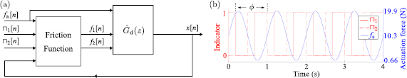
Figure 6. (a) Block diagram of the discrete-time model employed in the numerical simulations. The plant 
 is the discretized version of
  . The friction function block computes the friction forces f 1[n] and f 2[n] using the algorithm in (5) and the inputs
 ![$\sqcap_1[n]$](https://content.cld.iop.org/journals/1748-3190/14/3/036004/revision2/bbaae7bbieqn096.gif) ,
, ![$\sqcap_2[n]$](https://content.cld.iop.org/journals/1748-3190/14/3/036004/revision2/bbaae7bbieqn097.gif) ,
, ![$f_{\rm a}[n]$](https://content.cld.iop.org/journals/1748-3190/14/3/036004/revision2/bbaae7bbieqn098.gif) and x[n]. Zero initial conditions are set to start the simulations. (b) Example input signals. In this case, the central actuation force,
and x[n]. Zero initial conditions are set to start the simulations. (b) Example input signals. In this case, the central actuation force,  , is modeled as a sinusoidal wave with its magnitude and bias consistent with the empirically-estimated internal pressures of the central actuator during periodic operation (see the appendix). Specifically,
  is set to oscillate between
  and
and  . The indicator function
 ![$\sqcap_i[n]$](https://content.cld.iop.org/journals/1748-3190/14/3/036004/revision2/bbaae7bbieqn103.gif) , for
, for  , switches the friction of the corresponding actuator i from high (
![$\sqcap_i[n]=1$](https://content.cld.iop.org/journals/1748-3190/14/3/036004/revision2/bbaae7bbieqn105.gif) ) to low (
) to low (![$\sqcap_i[n]=0$](https://content.cld.iop.org/journals/1748-3190/14/3/036004/revision2/bbaae7bbieqn106.gif) ), and vice versa. In this case, high friction corresponds to
), and vice versa. In this case, high friction corresponds to  (or
(or  ) and low friction corresponds to
  (or
(or  ). The frequencies of all the inputs are set to
  (
( ) and the phase difference between the extremal actuators is set to
  (equivalent to
  ).
).
Download figure:
Standard image High-resolution imageDuring the execution of the simulations, at each computational step, the algorithm running inside the FFB evaluates the displacement and velocity outputs from  to determine the type and values of the instant frictional forces acting on the two extremal actuators. Specifically,
  , for
, for  , is set to
  , which implies that when the simulated speed
 ![$v_i[n]$](https://content.cld.iop.org/journals/1748-3190/14/3/036004/revision2/bbaae7bbieqn121.gif) , for
, for  , lies in the range
  , the associated mass i is considered to be static and
  is compared to
  to determine the value of
 ![$f_i[n]$](https://content.cld.iop.org/journals/1748-3190/14/3/036004/revision2/bbaae7bbieqn126.gif) according to (5). On the other hand, when
according to (5). On the other hand, when ![$\left| v_i [n] \right| \geqslant v_{{\rm s},i}$](https://content.cld.iop.org/journals/1748-3190/14/3/036004/revision2/bbaae7bbieqn127.gif) , the friction force acting on the mass i is immediately considered to be of the kinetic type. Also, in agreement with the empirical relationship between
, the friction force acting on the mass i is immediately considered to be of the kinetic type. Also, in agreement with the empirical relationship between  and
and  discussed above, for the implementation and execution of the simulation we define
for  . Considering the experimentally-identified mechanical characteristics of the central axial actuator presented in [30], we model the magnitude of the force generated by a cyclic inflation–deflation process,
  , using a biased sinusoidal signal with its amplitude and bias estimated from the minimum and maximum internal measured pneumatic pressures of actuation. Specifically, for simulation purposes we set the internal pressure of the central actuator to oscillate between
  and
and  , which in agreement with (1) translates to a force value that oscillates between
  and
and  ; a sample
  signal is shown in figure 6(b).
In the simulations, we limit the frequencies of all the inputs to be less than or equal to  . This parameter selection reflects the observed behaviors of the robot's actuators during real-time experiments. While the frequencies of the indicator signals,
 ![$\sqcap_1[n]$](https://content.cld.iop.org/journals/1748-3190/14/3/036004/revision2/bbaae7bbieqn138.gif) and
and ![$\sqcap_2[n]$](https://content.cld.iop.org/journals/1748-3190/14/3/036004/revision2/bbaae7bbieqn139.gif) , that determine the instantaneous friction forces are kept constant, they are set apart by a phase difference
, that determine the instantaneous friction forces are kept constant, they are set apart by a phase difference  which is actively varied between
  and
and  . The stiffness constant k is set to
  , which is the value estimated from a series of tensile tests conducted on a detached central actuator using an Instron Universal Testing Machine (Instron 5567). Also, a damping coefficient
  was implemented to account for energy dissipation; with this value, in agreement with empirical observations, the simulation results show that high-frequency displacement oscillations are mostly eliminated. All the simulations discussed in this paper were performed employing the fixed-step 4th-order Runge–Kutta method.
A set of simulation results, obtained with the parameters k, c,  ,
,  ,
,  and
and  (for
(for  ) selected above, are presented in figure 7. Here, figures 7(a) and (b) show the displacements and velocities of the two blocks for
  , the frequencies of
 ![$f_{\rm a}[n]$](https://content.cld.iop.org/journals/1748-3190/14/3/036004/revision2/bbaae7bbieqn151.gif) ,
, ![$\sqcap_1[n]$](https://content.cld.iop.org/journals/1748-3190/14/3/036004/revision2/bbaae7bbieqn152.gif) and
and ![$\sqcap_2[n]$](https://content.cld.iop.org/journals/1748-3190/14/3/036004/revision2/bbaae7bbieqn153.gif) set to
set to  and a phase difference
  . The instantaneous
  is calculated according to (4), compared to x1 and x2, and used to quantify the amount of locomotion. In the example of figure 7(a), the system covers a total distance of approximately
  in
in  , which corresponds to an average velocity of
  . Overall, the displacements of both masses follow a trajectory composed of a linear component and a periodic oscillation, while the position of
  varies according to a staircase-like pattern. The corresponding instant velocities of both masses exhibit periodic oscillation patterns. Interestingly, it can be observed that in this simulation to generate forward locomotion, both blocks slide simultaneously in opposite directions. Note that this resulting locomotion pattern is different from that commonly observed in the gaits of earthworms in which a segment firmly anchors before its adjacent segment moves forward.
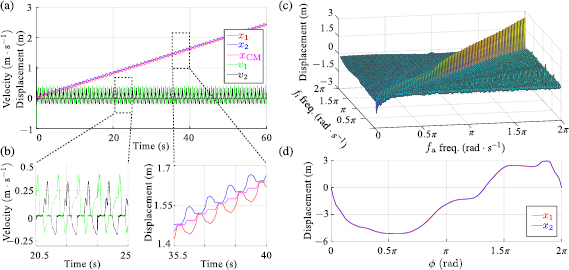
Figure 7. (a) and (b) Time-series of the robot's state and associated close-ups. These plots show the positions and velocities of the two extremal actuators when the input frequencies and  are set to
  and
and  , respectively. The displacement of the center of mass
  is also shown in magenta, calculated post-simulation according to (4). (c) Simulated displacement of block 1. This 3D-plot shows the position reached by the mass m1 after
  of locomotion when the constant frequencies of the actuation force (
 freq.) and friction input (f i freq., for
  ) are taken from the interval
 ![$\left[0.02\pi~\colon2 \pi \right]{\rm rad}\cdot{\rm s}^{-1}$](https://content.cld.iop.org/journals/1748-3190/14/3/036004/revision2/bbaae7bbieqn168.gif) while
while  is maintained at
  . (d) Experimental relationship between displacement and phase difference of the extremal actuators. The simulated positions x1 and x2 after
  are plotted over the
  interval
 ![$\left[0~\colon 2 \pi \right]{\rm rad}$](https://content.cld.iop.org/journals/1748-3190/14/3/036004/revision2/bbaae7bbieqn173.gif) . All the input frequencies are set to
. All the input frequencies are set to  while the phase difference
  is taken from the interval
 ![$\left[0~\colon 2 \pi \right]{\rm rad}$](https://content.cld.iop.org/journals/1748-3190/14/3/036004/revision2/bbaae7bbieqn176.gif) and
and  .
.
Download figure:
Standard image High-resolution imageFigure 7(c) shows the observed relationship between the input frequency and the amount of motion for the proposed pattern of actuation. Here, for  and
and  , the numerical simulation was repeatedly performed across a wide range of frequency combinations of the actuation force input
  (
( ) and the friction inputs f 1 and f 2 (
 ). Note that in all the cases, the frequencies of
 ![$\sqcap_1[n]$](https://content.cld.iop.org/journals/1748-3190/14/3/036004/revision2/bbaae7bbieqn183.gif) and
and ![$\sqcap_2[n]$](https://content.cld.iop.org/journals/1748-3190/14/3/036004/revision2/bbaae7bbieqn184.gif) are identical. The simulated displacements of the block 1 after
are identical. The simulated displacements of the block 1 after  of operation are plotted along the z-axis. This result strongly suggests that the selection of the input frequencies plays an essential role in locomotion generation and efficiency. Specifically, for inputs of this form, it is clear that substantial locomotion is achieved when the frequencies of all the inputs are closely matched. Also, in general, actuation inputs with higher frequencies generate faster locomotion. To demonstrate the relationship between the phase
 ![$\phi \in \left[0~\colon2\pi \right]~{\rm rad}$](https://content.cld.iop.org/journals/1748-3190/14/3/036004/revision2/bbaae7bbieqn186.gif) and velocity of locomotion, figure 7(d) shows the displacements x1 and x2 after
and velocity of locomotion, figure 7(d) shows the displacements x1 and x2 after  of operation, for all the input signals synchronized at
  (
( ) and
) and  . This result indicates that
  is crucial for locomotion generation and that its modulation can be directly employed to induce direction reversal. Even though these findings are limited to the specific actuation pattern and set of inputs employed in the discussed cases, they clearly exemplify the challenges and potentials of friction-controlled locomotion. The systematic characterization of the relationship between the robot's parameters and locomotion velocity, as well as the identification of the reachable subspace of the state-space x[n] with physically feasible inputs, is a matter of further research.
6. Real-time locomotion control experiment
6.1. Locomotion planning
In the previous section, we showed that high-performance locomotion can be achieved by employing perfectly-shaped periodic driving and frictional forces with closely matched frequencies. These conditions are not yet realizable with the pneumatically driven soft actuators designed and fabricated as shown in figure 4. Thus, the replication of the high-speed simulated locomotion behaviors using the physical robot is, at this moment, not an attainable objective. Consistently, to enable the robot to crawl, we implement a real-time strategy compatible with low actuation frequencies. This locomotion mode closely emulates earthworms' peristalsis-based crawling and can be readily applied to similar modular systems. From figure 5 it immediately follows that the block m1 remains stationary while the block m2 slides, as the central actuator inflates, if

In this case, the signal f 1 corresponds to static friction and f 2 corresponds to kinetic friction. Similarly, the block m2 stays anchored to the ground and the block m1 slides forward, as the central actuator deflates, if

In this case, the signal f 2 corresponds to static friction and f 1 corresponds to kinetic friction. Thus, forward locomotion can be generated by alternately activating the conditions described by (15) and (16). Similarly, backward locomotion can be realized by simply reversing the conditions defined in (15) and (16). In this way, a complete stride (forward or backward) can be generated by implementing a four-phase actuation sequence; figure 8 illustrates the forward motion case. Here, following the biological terminology on earthworm kinematics reviewed in section 2, we define the protrusion time as the span during which the central actuator expands (phase 2). Similarly, the stance time is defined as the span within a locomotion cycle during which the central actuator is not expanding. Note that during the stance time, the front actuator remains horizontally static while completing an inflation–deflation cycle ( ).
).

Figure 8. Actuation sequence employed to generate forward locomotion on a flat surface. Here, red indicates inflation and gray deflation; the 3D-printed casings are shown in sectional views so that the state of each actuator can be clearly seen in each phase of the locomotion sequence. When both extremal actuators are deflated, the smooth 3D-printed casings are in direct contact with the supporting surface and support the entire weight of the robot. To crawl forward, in phase 1, the back actuator is inflated and anchors to the ground; in phase 2, the central actuator is inflated to expand forward while the back actuator remains anchored to the ground; in phase 3, the front actuator is inflated and anchors to the ground; finally, in phase 4, both the back and central actuators are deflated and contract in order to complete a locomotion cycle.
Download figure:
Standard image High-resolution image6.2. Experimental results and discussion
A set of real-time experiments was conducted to validate the proposed locomotion method. The real-time locomotion control strategy is based on the implementation of a pressure tracking controller for each actuator. In this scheme, the reference pressure signal for each controller is determined off-line through an actuator characterization process. The details of the procedure and the corresponding experimental setup are presented in the appendix. Sets of experimentally-determined actuator pressure references corresponding to feasible forward and backward crawling motions are shown in table 1; the resulting controlled actuator pressure outputs for desired protrusion and stance times of  and
and  are shown figure 9. Here, it can be seen that the three actuators can track their prescribed reference pressures reasonably well. Unlike the forward case, during backward crawling, the stance time is given by the span during which the back actuator remains stationary with respect to the flat supporting surface after the central actuator has been fully inflated. The protrusion and stance states corresponding to backward locomotion are defined exactly as in the forward case. As an example, the photographic sequence in figure 10 shows stills from a movie in which the robot performs bidirectional crawling on a horizontal flat HDPE surface. The complete experiment is shown in the supporting movie BBS1.mp4.
Table 1. Reference pressures during actuation (kPa).
| Phase | 1 | 2 | 3 | 4 | |
|---|---|---|---|---|---|
| Forward locomotion | Front actuator | 0 | 0 | 8.6 | 8.6 |
| Central actuator | 0 | 19.3 | 19.3 | 0 | |
| Back actuator | 7.6 | 7.6 | 7.6 | 0 | |
| Backward locomotion | Front actuator | 8.6 | 8.6 | 8.6 | 0 |
| Central actuator | 0 | 19.3 | 19.3 | 0 | |
| Back actuator | 0 | 0 | 7.6 | 7.6 | |
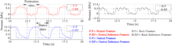
Figure 9. Pressure signals of the robot's actuators during a forward locomotion test. From the upper-left (in red) to the bottom-left (in blue) to the upper-right (in black) the plots show the references (F-RP, C-RP and B-RP) and controlled outputs (F-P, C-P and B-P) of the front, central and back actuators. In this case, the protrusion time is  , the stance time is
  and corresponding stride time is
  .
.
Download figure:
Standard image High-resolution image
Figure 10. Photographic sequence composed of movie stills showing the soft robot crawling bidirectionally on a flat HDPE surface. During this test, the traveling direction is reversed every  and the forward and backward locomotion is implemented employing the actuator pressure references listed in table 1. The complete experiment can be found in the supporting movie BBS1.mp4.
Download figure:
Standard image High-resolution imageFor purposes of analysis, the experimental locomotion data is extracted and processed using Open Source Computer Vision (OpenCV). Figure 11(a) presents the displacement history of the robot during the bidirectional crawling experiment in figure 10, which were obtained by tracking and processing the left edges of both yellow casings. A close-up of the estimated motion signals clearly demonstrates the working principle of the robot, as it can be observed that the front and back actuators are controlled to alternately anchor (stick) and slide (slip), according to the conditions defined in (15) and (16). In this experimental test, the robot is controlled to reverse its direction every  . During forward locomotion, the stride length is approximately
  with an average speed of
  (HDPE-F in table 2). During backward locomotion, the stride length is approximately
  with an average speed of
  (HDPE-B in table 2).

Figure 11. (a) Trajectories of the extremal actuators during the bidirectional locomotion test. The time-series corresponding to the back block is shown in red; the time-series corresponding to the front block is shown in blue. The direction of locomotion is reversed every  ; a zoomed-in view of one of the controlled reversals (from
  to
to  ) is shown in the superposed window. (b) Trajectories of the extremal actuators of the robot while climbing on the HDPE surface held at a 7.5° angle with respect to the horizontal. The time-series corresponding to the back block is shown in red; the time-series corresponding to the front block is shown in blue.
Download figure:
Standard image High-resolution imageTable 2. Experimental results on horizontal surfaces.
| Surface material | Stride period (s) | Stride length (m) | Speed ( ) ) |
|---|---|---|---|
| HDPE-F | 3 | 0.028 | 0.0089 |
| HDPE-B | 3 | 0.022 | 0.0070 |
| Benchtop | 3.5 | 0.027 | 0.0067 |
| Wood | 3 | 0.012 | 0.0038 |
| Foam | 3 | 0.016 | 0.0054 |
| Aluminum | 3.5 | 0.021 | 0.0058 |
| Foam + HDPE | 3.5 | 0.021 | 0.0058 |
The discrepancy between the forward and backward speeds is caused by a noticeable difference between the amount of slippage experienced by the front actuator when sliding in different directions, most likely due to fabrication errors. Also note that, as seen in table 1, the front actuator requires a higher internal pressure threshold than the back actuator to create a firm contact with the supporting surface. The observed inverse correlation between the amount of displacement generated by the robot and unwanted slippage is in agreement with the findings in [36]. Employing the same actuation sequence in figure 8 and parameters in table 1, the robot is thoroughly demonstrated to crawl effectively on several surfaces with different associated friction coefficients, including a laboratory benchtop, wood, a foam pad and aluminum (see supplementary movie BBS1.mp4). In addition, we show that the robot is capable of transitioning between surfaces with different coefficients of friction; for example, from a foam pad to an HDPE plate, as can be seen in BBS1.mp4.
The relevant OpenCV-estimated locomotion parameters corresponding to these experimental tests are summarized in the last five rows of table 2. Note that different stride periods are required for the robot to adapt and achieve robust crawling on different types of surfaces. For consistency of analysis, the recorded speed is that of the system's center of mass and for the case in which the robot crawls from a foam pad to an HDPE plate (Foam + HDPE), only the time spans during which both extremal actuators are on a given surface are employed in the estimation of the locomotion parameters. Among all the tested surfaces, the slowest speed is obtained when the robot crawls on wood, probably because microscopic timber particles accumulate on the silicone surfaces of the actuators, thus altering the corresponding friction coefficients and progressively causing more undesired slippage.
To assess the ability of the robot to travel on inclined surfaces, we performed a set of tests using the same parameters in table 1 but with the robot crawling upward on an HDPE plane positioned at a  angle with respect to the ground. In these tests, the protrusion and stance times, as in the horizontal cases, were set to be
  and
and  , respectively. The plot in figure 11(b) shows the OpenCV-estimated positions of the left-bottom corners of both yellow casings and a photographic sequence of the experiment is displayed in figure 12. In this case, the robot achieves a stride length of approximately
  and an average speed of
  . It can be observed that the downward components of the gravitational forces acting on the casings and the steel plates induce shear forces that cause the anchored extremal actuators to bend and curl. Thus, the contact areas between the actuators and the inclined plane are reduced, which noticeably increases the slippage at both ends of the robot. As in the horizontal cases, slippage appears to affect more severely the front actuator than the back actuator. The complete set of inclined experimental tests can also be found in the supporting movie BBS1.mp4.
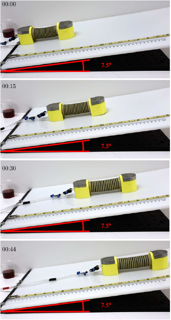
Figure 12. Photographic sequence composed of movie stills showing the soft robot climbing on an inclined HDPE surface positioned at an angle of  with respect to the horizontal. A cup containing dyed water indicates the direction of the gravitational force. The complete experiment can be found in the supporting movie BBS1.mp4.
Download figure:
Standard image High-resolution imageThrough the experiments presented in this section, we clearly demonstrated the suitability and effectiveness of the proposed friction-controlled scheme for generating bidirectional peristalsis-based crawling using the robot introduced in section 2. Note that the locomotion speeds observed in the experiments are not comparable to those obtained in the numerical simulations. This discrepancy is expected because the actuation methods adopted in both types of implementations are substantially different. In the experimental cases, locomotion control is achieved indirectly by modulating the deformation of the actuators via feedback control of their internal air pressures; in the simulations, the locomotion modes are directly controlled. Direct displacement control of the robot will be implemented in the future by employing faster actuators and a real-time motion-capture system as the main sensor in a feedback loop. Finally, it is important to emphasize that the main characteristic of the locomotion approach introduced in this work is that, unlike existing methods based on anisotropic friction, the actuator switching mechanisms enable active control of the isotropic frictions between the actuators and contacting surface; thus, the basic design of the robotic prototype in figure 1 can be readily modified to create active steering capabilities by simply enabling the central actuator to bend and twist and not only extend and contract. Furthermore, note that the structural configuration of the proposed robot enables the adoption of other mechanisms for the generation of traction and anchoring forces, such as suction and magnetism, to make possible locomotion on flat perpendicular or uneven surfaces.
7. Conclusions and future work
We presented the design, fabrication and control of an earthworm-inspired crawling soft robot capable of bidirectional locomotion on both horizontal and inclined flat surfaces. The robot is composed of pneumatic actuators made of silicone rubber and 3D-printed casings, designed to jointly emulate the functionalities of an earthworm's longitudinal and circular muscles as well as the bristle-like setae structures employed to modulate traction. Locomotion is generated and controlled through the active switching of the robot's surfaces in contact with the supporting ground, and thus the corresponding coefficients of friction, while a main central actuator provides mechanical power periodically. In this approach, the central actuator and friction switching mechanisms are actuated by coordinated inflation–deflation sequences. For the purposes of analysis and control, we modeled the robot as a double-mass-spring-damper system and described its crawling dynamics using a reduced-complexity LTI state-space representation. Employing this model, we proved mathematically that in the absence of friction, systems of the type considered here (figure 1) cannot locomote or be controlled; and consistently, that frictional forces can be used as inputs to generate and control locomotion. This finding was thoroughly validated through numerical simulations and real-time control experiments.
The design of the robot in figure 1 is highly versatile as it can be thought of as a two-metamere-inspired module. Thus, complex robotic configurations can be created by assembling independent actuation modules with distinct and complementary functionalities, which is a matter of further research partly inspired by the concepts and ideas in [52, 53]. In agreement with this vision, we anticipate the development of scalable multi-module robots with steering capabilities and locomotion modes adaptable to uneven terrains and steep inclines. In this context, complex large multi-module configurations are ideal platforms for developing and testing novel decentralized control strategies, which are necessary to optimize the distributed placement of sensors and actuators in the system. Also, from the dynamic modeling perspective, we envision the possibility of characterizing the repeating wave-like gait of large modular configurations using coupled oscillators [54]. This approach has the potential to enable the development of bio-inspired controllers based on the concept of central pattern generator (CPG). Finally, we anticipate substantial research on new power technologies for actuation as full autonomy will be achieved only when portable high-density sources of energy are developed. Feasible options for soft robots of the type discussed here include pulsed gas-phase combustion and catalytic-combustion-driven SMA-based artificial muscles, which are matters of both current and further research.
Acknowledgments
This work was partially supported by the National Science Foundation (NSF) through CMMI Award 1833497 and the Chilean National Office of Scientific and Technological Research (CONICYT) through a graduate fellowship to A A Calderón. Additional support was provided by the USC Viterbi School of Engineering through a startup fund to N O Pérez-Arancibia and graduate fellowships to J Z Ge, A A Calderón and L Chang.
Appendix
To drive the robotic system, an Elemental O2 commercial air pump and a 12-V ROB-10398 vacuum pump are employed to inflate and deflate the three actuators through a manifold (SMC VV3Q12). Three Honeywell ASDX Series silicon pressure sensors and three high-speed normally-closed solenoid valves (SMC VQ110-6M) are used to measure and regulate the air internal pressure of each actuator. The tasks of data acquisition and signal processing are performed using a National Instruments PCI-6229 data acquisition (DAQ) board mounted on a target PC which communicates with a host PC as part of a xPC Target 5.5 configuration setup (MATLAB R2013b). In this scheme, three digital proportional-integral-derivative (PID) controllers,  , for
, for  , control the internal pressure of each actuator with associated discrete-time dynamics Pi(z), for
  , according to the feedback loop in figure A1.

Figure A1. LTI scheme used to independently control each actuator ( ) of the soft robot. Here, the discrete-time plant Pi(z) represents the entire SISO dynamics of the actuator i, including those associated with the corresponding inflatable silicone-rubber structure, pressure sensor, solenoid valve and DAQ board. The input to Pi(z) is the duty cycle of the PWM signal that opens and closes the corresponding solenoid valve;
  is the measured internal air pressure;
  is the reference pressure; and
  is the PID controller that controls the internal air pressure of the corresponding actuator i.
Download figure:
Standard image High-resolution image
During actuation, both the inflation and exhaust pumps are maintained at constant flow rates and output pressures; for each actuator, the net air flow and internal pressure are manipulated by the fast solenoid valves using pulse width modulation (PWM). Accordingly, each plant Pi(z) represents the entire combined SISO dynamics of the actuator i, including those associated with the corresponding inflatable structure, solenoid valve, pressure sensor and DAQ board. The input to Pi(z) is the duty cycle of the PWM that opens and closes the corresponding solenoid valve, and the output from Pi(z) is the measured pressure value  . The difference between the reference pressure
  and
and  is the input to the corresponding controller
  , as shown in figure A1.
The experimental characterization process of the robot is based on the procedure introduced in [30]. Consistently, to identify the relationship between the internal pressure and elongation of the central longitudinal actuator, a set of inflation–deflation experiments were conducted in order to measure the relevant pressure-elongation data points in a predefined set, without causing significant radial expansion of the test actuator. In the case of the extremal actuators, the minimum pressure thresholds required to establish a firm contact with the supporting surface were found through visual observation. The information obtained from the system characterization experiments is employed to determine the actuator pressure references  required to implement the four-phase actuation locomotion sequence in figure 8 (see table 1), employing the simple PID control scheme in figure A1. As discussed in section 6, this approach was demonstrated to be greatly effective to generate friction-controlled bidirectional locomotion.
Footnotes
- *
Preliminary results of this work were presented at the 2017 IEEE International Conference on Robotics and Biomimetics (ROBIO 2017).