

Abstract
Herbivory is an important part of most ecosystems and affects the ecosystems' carbon balance both directly and indirectly. Little is known about herbivory and its impact on the carbon balance in high arctic mire ecosystems. We hypothesized that trampling and grazing by large herbivores influences the vegetation density and composition and thereby also the carbon balance. In 2010, we established fenced exclosures in high arctic Greenland to prevent muskoxen (Ovibos moschatus) from grazing. During the growing seasons of 2011 to 2013 we measured CO2 and CH4 fluxes in these ungrazed blocks and compared them to blocks subjected to natural grazing. Additionally, we measured depth of the water table and active layer, soil temperature, and in 2011 and 2013 an inventory of the vegetation density and composition were made. In 2013 a significant decrease in total number of vascular plant (33–44%) and Eriophorum scheuchzeri (51–53%) tillers were found in ungrazed plots, the moss-layer and amount of litter had also increased substantially in these plots. This resulted in a significant decrease in net ecosystem uptake of CO2 (47%) and likewise a decrease in CH4 emission (44%) in ungrazed plots in 2013. While the future of the muskoxen in a changing arctic is unknown, this experiment points to a potentially large effect of large herbivores on the carbon balance in natural Arctic ecosystems. It thus sheds light on the importance of grazing mammals, and hence adds to our understanding of natural ecosystem greenhouse gas balance in the past and in the future.
Export citation and abstract BibTeX RIS

Content from this work may be used under the terms of the Creative Commons Attribution 3.0 licence. Any further distribution of this work must maintain attribution to the author(s) and the title of the work, journal citation and DOI.
1. Introduction
Half of the Earth's land surface is influenced by large herbivores (livestock or native) (Olff et al 2002), and their presence may have great influence on the ecosystem (e.g. Mulder 1999, Tanentzap and Coomes 2012). In the Arctic, herbivory has been shown to influence the carbon cycle (e.g. Van der Wal et al 2007, Sjögersten et al 2011, Cahoon et al 2012, Falk et al 2014). The presence or absence of herbivores may determine whether the system is a net carbon source or sink (Welker et al 2004, Sjögersten et al 2011). Nonetheless, the general impact of grazing on the carbon balance appears somewhat ambiguous. The contrasting results may be related to ecosystem type and grazing pressure. Grazing can also change nutrient and carbon allocation patterns within plants, as vegetation uses carbon and nutrients reserves to regrow new plant shoots instead of building below-ground reserves (e.g. Chapin 1980, Mulder 1999, Falk et al 2014). Herbivore trampling suppresses moss and shrub growth, their grazing keeps the litter layer to a minimum and their manure fertilizes the soil; thus, with a decline in herbivory, landscapes may undergo succession from open land to woodland or shrubland (Zimov et al 1995). Supporting this theory, grazing in the arctic may result in the vegetation shifting towards more herb and graminoid dominance (e.g. Post and Pedersen 2008, Sjögersten et al 2008, Cahoon et al 2012, Vaisanen et al 2014).
Compared to other arctic habitats, mires are highly productive and they are an important source of forage for many herbivore species (Henry et al 1990, Henry 1998, Forchhammer et al 2008, Kristensen et al 2011). Arctic wetlands hold large amounts of carbon, as the decomposition rate of organic matter is slow under cold and anoxic conditions (Tarnocai et al 2009). Natural and agricultural wetlands together contribute with more than 40% of the annual atmospheric emissions of CH4 and are considered the largest single contributor of this gas to the troposphere (Cicerone and Oremland 1988, Mikaloff Fletcher et al 2004). Despite the likely impact herbivory may have on the carbon balance in arctic wetlands and on the controlling aspects for CH4 production and emission, only very few studies have focused on herbivory and CH4 fluxes in the arctic or sub-alpine regions (Sjögersten et al 2011, 2012, Falk et al 2014). We recently showed that a simulated increased grazing pressure resulted in a more than 25% decrease in CH4 emission in a high arctic mire (Falk et al 2014). This, however, contrasts with the findings of other studies (Sjögersten et al 2011, 2012) that showed no effect of herbivory on CH4 emissions. Many of the factors that influence both CO2 and CH4 fluxes either directly or indirectly are influenced by herbivory. These include soil temperature and water table depth (Torn and Chapin 1993, Waddington et al 1996) and vegetation composition and density (Ström et al 2003, 2012, Ström and Christensen 2007). Hence, to understand the effect of herbivory on the total carbon balance of the artic, it is crucial to understand the potential impact it has on both CO2 and CH4 fluxes.
Here we focus on how the vegetation composition and the carbon balance are affected when muskox grazing is excluded from parts of an arctic mire. In Falk et al (2014) we found indications that increased simulated grazing resulted in a decrease in the total number of vascular plant and Eriophorum tillers and, as described above, in CH4 emission. We consequently hypothesize that exclusion of muskoxen will: (1) change the composition and density of the vegetation, with an increase in the number of vascular plant tillers (see Falk et al 2014), which in turn (2) will lead to an increase in net ecosystem exchange (NEE), gross primary production (GPP) and CH4 emission. In order to test our hypotheses, we utilized a herbivore exclusion experiment installed in high arctic mire in 2010. To be able to exclude that the fences of the exclosures had an effect on the snow density and thereby the reason for a potential change, snow control plots were installed. We expect to see no differences between control and snow control plots as the mesh size of the fence is 10 × 10 cm. Between 2011 and 2013, we measured CO2 and CH4 fluxes and several additional properties (soil temperature, active layer and water table depth and vegetation composition and density).
2. Materials and methods
2.1. Site description
The study took place in the Zackenberg valley, NE Greenland (74°30'N 20°30 W). The warmest month (July) has a mean monthly air temperature of 5.8 °C. The mean annual precipitation was 260 mm in the period 1996–2005, mainly falling as snow (Hansen et al 2008). The valley is underlain by continuous permafrost, and the active layer thickness varies from 45 to 80 cm depending on the type of ecosystem (Christiansen et al 2008). Mires cover approximately 4% of the valley (Arndal et al 2009) and are dominated by a few vascular plant species (see table 2) and a dense moss cover.
The muskox (Ovibos moschatus), the only large herbivore in NE Greenland, is a natural part of the ecosystem throughout the year, and around 80% of their graminoid-dominated summer forage is obtained in the mire areas (Kristensen et al 2011). In the summer the muskoxen are usually found in densities of 1–2 individuals per km2 in the 47 km2 census area in the Zackenberg valley (Schmidt et al 2015). This number increases to approximately seven individuals per km2 in late summer and autumn when they gather in the mire and grassland areas to forage (Schmidt et al 2015). With a changing climate, the future of muskoxen in NE Greenland is hard to predict. The population size of muskoxen depends on the biomass production and the length of the growing season; a long growing season will increase the number of muskoxen the following year (Forchhammer et al 2008). However, with predicted increasing numbers of thaw days during winter (Stendel et al 2008), which can lead to ice crust formation, a decline in the muskox population is very likely. Hard and deep snow cover is known to increase the mortality of muskoxen during the winter, as they may not be able to access the vegetation (Forchhammer et al 2002).
2.2. Experimental setup
In July 2010, permanent muskox exclosures were established in the mire in Zackenberg. The experiment consists of five replicate blocks, each including the following three 10 × 10 m areas (n = 15): (1) an un-manipulated control area (C). (2) An exclosure area (EX) where a one meter high standard sheep fence prevents muskoxen from grazing and trampling. (3) A snow control area (SC), fenced towards NNW (the dominant wind direction in (Hansen et al 2008)), to evaluate the potential effect of the fence on snow depth. Muskoxen can move and graze freely in C and SC. The blocks are located on a slight downhill slope that is water-saturated in the beginning of the growing season, while it often dries out later in the season. Blocks 1 and 2 are positioned farthest uphill in a drier part of the mire while blocks 3, 4 and 5 are further downstream in a wetter and flatter part. Blocks 3, 4 and 5 have similar water table depths but the peat layer in block 5 is lower and in addition mixed with silt.
In 2010 two measurement plots (39.5 × 39.5 cm) were permanently installed inside each of the 15 areas (n = 30). In 2011, one additional control area was added in blocks 3 and 4, due to large differences in vegetation composition between the initial C, EX and SC areas in these blocks. The theoretical reason for these additions was our previous findings, which showed that the vascular plant species composition is of great importance for CH4 fluxes (Ström et al 2003, 2012) rendering an analysis of change impossible between plots with a large difference in initial conditions. A total of 11 plots were installed outside and inside EX 3 and EX 4 giving a total of 41 measurement plots. Each plot consisted of an aluminum frame that was fitted 15 cm into the ground. On all plots we measured gas fluxes and additional parameters at least once per week over the main part of the growing seasons. To enable a more detailed study of CH4 fluxes, all variables were measured more frequently (approximately twice per week) in blocks 3 and 4. Details on measurement procedure are further described in Falk et al (2014). The timing of the measurement periods are summarized in table 1.
Table 1. The measuring period for CO2 and CH4 fluxes in 2011, 2012 and 2013, and the number of flux measurements done each month.
| Measuring period | June | July | August | September | October | |
|---|---|---|---|---|---|---|
| CO2 | ||||||
| 2011 | 30 June–8 August | 0–1 | 4–5 | 1 | ||
| 2012 | 6 July–7 September | 3–4 | 3–4 | 1 | ||
| 2013 | 2 July–17 august | 4 | 2 | |||
| CH4 | ||||||
| 2011 | 5 July–8 August | 8 | 2 | |||
| 2012 | 7 July–6 October | 6 | 6 | 5 | 2 | |
| 2013 | 1 July–17 August | 7 | 4 |
2.3. Measurements
To estimate the density and composition of vascular plants, the number of tillers per plot of the dominant plant species were counted, on all 41 plots in 2013 and in blocks 3, 4 and 5 (n = 26) in 2011. In mid-August 2013, biomass was harvested, directly below the fresh moss layer, within a 0.40 m2 square randomly placed in close proximity to the measuring plots within each block and treatment (n = 15). Each sample was divided into biomass of Carex, Dupontia, Eriophorum and fresh mosses and the dry weight of the fraction was determined after drying the samples at 60 °C for 48 h. In each of the vascular plant fractions we measured the mean tiller height and counted the number of plant tillers and green leaves.
Gas concentrations of CO2 and CH4 were recorded simultaneously by a portable FTIR (Fourier transform infrared) spectrometer (Gasmet Dx 40-30, Gasmet Technologies Oy, Finland) within a transparent Plexiglas chamber (41 L). The concentration change of CO2 in the chamber during light conditions was used to estimate NEE and during dark to estimate ecosystem respiration (Reco). Each block was measured within one day to minimize effects of changes in weather conditions. Release of gas from the ecosystem to the atmosphere is denoted by positive values and uptake by negative. Variables measured in addition to gas fluxes were water table depth (WtD, cm below moss surface), the active layer thickness (AL, cm below moss surface) and soil temperature (Ts, 10 cm below moss surface). These measurements were done within or in close proximity to the respective plot. See Falk et al (2014) for further details on the methodology.
At end of winter in 2012, we measured the snow depth in all treatments in all blocks. Approximately 12 measurements were conducted within each treatment plot using a handheld magna-probe. The total number of data points included thus equaled 174.
2.4. Data analysis
Only the most dominating plant species (Arctagrostis, Carex, Dupontia, Eriophorum and Equisetum) and the total number of these species were included in the data analysis. The density of tillers per m2 (vegetation analysis) was normal distributed for all species except for Carex and Equisetum. A nonparametric (Kendall's) test with related samples and an independent t-test were tested and showed similar results. Hence, an independent t-test was used to test for differences in vegetation parameters between C, EX and SC. Two separate analyses were performed; one on the whole dataset (n = 26, n = 41 for 2011 and 2013, respectively) and one on the plots used in the CH4 analysis (n = 14). The harvested biomass samples were not normally distributed and a nonparametric (Kendall's) test with related samples was performed, where the block structure was considered in the model. Treatment effects on snow depth were examined using a mixed model approach, where treatment was regarded as fixed factor and block as random factor. Snow depth data were log-transformed prior to analyses. As a post-hoc test we used Tukey HSD tests (p < 0.05).
On all plots the CO2 and CH4 fluxes (mg m−2 h−1 of CH4 or CO2) were calculated from the change in gas concentration as a function of time using linear fitting, including corrections for ambient air temperature and pressure, according to procedures by Crill et al (1988). Due to a highly significant correlation (R = 0.947, p < 0.0001) between light and dark CH4 fluxes for individual plots, the mean of these two measurements was used in the CH4 flux analysis. GPP was calculated as the difference between NEE and Reco. In a previous study (Ström et al 2012) we made several attempts to de-trend data and remove diurnal and seasonal dynamics in CO2 using PAR and Ts, according to various linear and nonlinear methods (e.g., Lund et al 2009, Lindroth et al 2007). However, all these computations resulted in very low R2 values and the modeled data could not be used with confidence. In this study we refrained from correcting GPP and NEE due to these reasons.
The dataset for the gasfluxes was much larger (table 1) than for the vegetation analysis (one measurement per plot), which allowed a much more detailed statistical approach to be used. The effects of exclusion on the carbon flux were examined using general mixed linear models with treatment as fixed factor. Block and plot were regarded as random factors, and, to avoid pseudo-replication, plot nested within block. We included a Gaussian autoregressive component within plots in the models due to the expected temporal dependence in fluxes. The analysis was conducted using the PROC MIXED procedure (SAS Institute Inc. 2000). Model reduction was based on likelihood ratio tests and successive removal of non-significant variables (p > 0.05). As post-hoc test we used Tukey HSD tests (p < 0.05). The CO2 analysis included all plots (n = 41 plots) and the CH4 analysis only wet blocks (n = 14).
3. Results
Irrespective of treatment the vegetation analysis performed on the measurement plots in 2011 and 2013 showed a large spatial variation in vegetation composition within the area (table 2). In 2011 and 2013 the dominating species Arctagrostis, Carex, Dupontia, Eriophorum and Equisetum on average accounted for 99% of all vascular plant species, with Dupontia and Eriophorum being the most dominating (table 2). In 2011, no significant differences between any of the treatments were found with respect to the total density (number of tillers) of vascular plants or in the density of individual plant species in the plots. However, in 2013 the total density of vascular plants and Eriophorum were significantly lower in EX compared to C plots, while no significant differences were found between C and SC, although there was a tendency of Eriophorum to be lower in SC. When the tiller analysis was performed on the wet blocks used for the detailed CH4 analysis, the results were the same with no significant differences in 2011, but with significantly lower Eriophorum and total tiller densities in EX than in C areas in 2013, p = 0.008 and p = 0.001 for Eriophorum and total tiller densities, respectively. The treatment effects on tiller number were further confirmed in the samples harvested in 2013 (table 3): the number of both total vascular plants and Eriophorum tillers was also here significantly lower in EX than in C, while no significant differences between other species or between SC and C were found (table 3). In addition, the tiller analysis of the harvested samples showed that the number of total vascular plant and Eriophorum leaves that was green were significantly lower in EX than in C and that the tillers of Dupontia, Eriophorum and all vascular plants combined were higher in EX than in C. No significant differences were found between these fractions for the other dominant species or between C and SC (table 3).
Table 2. The mean, maximum, minimum and standard error of the mean (SE) of vascular plants tillers per m2 counted in measurement plots in control (C), exclosure (EX) and snow-control (SC) areas in 2011 (C n = 17, EX n = 14, SC n = 10) and 2013 (C n = 13, EX n = 10, SC n = 6). Samples were fractionated into vascular plants: Arctagrostis latifolia (Arctagrostis), Carex stans (Carex), Dupontia psilosantha (Dup), Eriophorum scheuchzeri (Erioph), Equisetum sp and total number of tillers (sum). Significant differences (independent t-test) between C and EX and C and EX are shown in bold formatting.
| Arctagrostis | Carex | Dupontia | Eriophorum | Equisetum | Sum | ||||||||||||||
|---|---|---|---|---|---|---|---|---|---|---|---|---|---|---|---|---|---|---|---|
| C | EX | SC | C | EX | SC | C | EX | SC | C | EX | SC | C | EX | SC | C | EX | SC | ||
| 2011 | Mean | 498 | 266 | 315 | 383 | 20 | 2057 | 2556 | 3263 | 1702 | 2700 | 1784 | 1869 | 904 | 734 | 1210 | 6136 | 5333 | 5944 |
| Max | 1588 | 1288 | 1369 | 3313 | 200 | 6163 | 4131 | 5125 | 5063 | 5219 | 3544 | 2981 | 5319 | 3375 | 4850 | 8869 | 7456 | 9225 | |
| Min | 0 | 0 | 0 | 0 | 0 | 0 | 0 | 750 | 0 | 31.3 | 188 | 669 | 0 | 0 | 0 | 2969 | 2700 | 1225 | |
| SE (±) | 142 | 139 | 231 | 275 | 20 | 1025 | 401 | 383 | 978 | 452 | 352 | 486 | 505 | 372 | 745 | 555 | 500 | 1376 | |
| p | 0.267 | 0.491 | 0.213 | 0.223 | 0.228 | 0.466 | 0.144 | 0.261 | 0.309 | 0.238 | 0.309 | 0.876 | |||||||
| 2013 | Mean | 153 | 58 | 69 | 84 | 60 | 394 | 1663 | 1378 | 1463 | 1280 | 627 | 946 | 24 | 16 | 14 | 3181 | 2122 | 2872 |
| Max | 881 | 188 | 394 | 700 | 488 | 1881 | 2813 | 2019 | 3013 | 2306 | 1094 | 1813 | 244 | 213 | 94 | 4163 | 2844 | 4075 | |
| Min | 0 | 0 | 0 | 0 | 0 | 0 | 0 | 106 | 0 | 544 | 188 | 419 | 0 | 0 | 0 | 2369 | 1438 | 1381 | |
| SE (±) | 54 | 19 | 38 | 47 | 42 | 216 | 173 | 155 | 385 | 120 | 64 | 152 | 15 | 15 | 19 | 137 | 113 | 361 | |
| p | 0.110 | 0.288 | 0.717 | 0.242 | 0.238 | 0.653 | 0.000 | 0.085 | 0.708 | 0.625 | 0.000 | 0.282 | |||||||
Table 3. The mean (±SE), maximum and minimum number of tillers and green leaves and average tiller height (cm) of the dominant vascular plant species and the sum of these in harvested biomass samples (0.04 m−2) in control (C), exclosure (EX) and snow-control (SC) areas (C n = 7, EX n = 5, SC n = 5). Samples were fractionated into vascular plants: Carex stans (Carex), Dupontia psilosantha (Dup), Eriophorum scheuchzeri (Erioph) and total number of tiller (total). Significant differences (nonparametric Kendall's test) between C and EX and C and EX are shown in bold formatting.
| Number of tillers | Number of green leaves | Height of tillers | |||||||||||
|---|---|---|---|---|---|---|---|---|---|---|---|---|---|
| Dup. | Carex | Erioph. | Total | Dup. | Carex | Erioph. | Total | Dup. | Carex | Erioph. | Mean | ||
| C | Mean | 69 ± 22 | 6 ± 1 | 79 ± 23 | 154 ± 15 | 108 ± 37 | 15 ± 5 | 110 ± 31 | 234 ± 25 | 10 ± 2.7 | 9 ± 0.9 | 11 ± 0.4 | 11 ± 0.5 |
| Max | 115 | 12 | 168 | 180 | 201 | 27 | 228 | 291 | 15 | 11 | 12 | 12 | |
| Min | 0 | 4 | 48 | 98 | 0 | 0 | 57 | 142 | 0 | 6 | 10 | 10 | |
| EX | Mean | 47 ± 16 | 4 ± 2 | 37 ± 7 | 87 ± 13 | 53 ± 18 | 6 ± 4 | 50 ± 11 | 108 ± 13 | 14 ± 3.6 | 5 ± 3.4 | 15 ± 0.9 | 15 ± 0.9 |
| Max | 88 | 10 | 57 | 109 | 101 | 23 | 86 | 143 | 19 | 16 | 17 | 18 | |
| Min | 0 | 0 | 21 | 40 | 0 | 0 | 22 | 68 | 0 | 0 | 12 | 13 | |
| p (C versus EX) | 0.180 | 0.180 | 0.025 | 0.025 | 0.180 | 0.317 | 0.025 | 0.025 | 0.046 | 0.655 | 0.025 | 0.025 | |
| SC | Mean | 49 ± 20 | 24 ± 23 | 48 ± 9 | 121 ± 21 | 66 ± 33 | 51 ± 47 | 64 ± 13 | 181 ± 48 | 8 ± 2.2 | 4 ± 2.7 | 10 ± 0.6 | 10 ± 0.5 |
| Max | 102 | 114 | 76 | 183 | 184 | 240 | 108 | 305 | 13 | 11 | 11 | 12 | |
| Min | 0 | 0 | 20 | 56 | 0 | 0 | 32 | 70 | 0 | 0 | 8 | 9 | |
| p (C versus SC) | 0.317 | 0.317 | 0.655 | 0.655 | 0.317 | 1.000 | 0.655 | 0.655 | 0.317 | 0.317 | 0.655 | 0.317 | |
The biomass (dry weight) of several of the fractions of the harvested samples were significantly (p < 0.03) higher in EX and SC than in C (figure 1). These included a higher total biomass (59% including all fractions), vascular plant litter (230%) and moss (55%) biomass in EX compared to C and a higher total biomass (15%) and moss (25%) biomass in SC than in C. No significant differences were found (p > 0.180) between C and EX or SC for any of the individual species, although the weight of the biomass of Dupontia tended to be higher in EX than in C (p = 0.083).

Figure 1. Mean dried biomass (g ± SE) fractions of samples harvested (0.04 m2) in August 2013 in controls (n = 7), exclosures (n = 5) and snow-controls (n = 5). Samples were fractionated into vascular plants: Carex stans, Dupontia psilosantha and Eriophorum scheuchzeri and fresh mosses, old biomass (Litter) and the total weight of the dried biomass (total biomass). Significant differences (nonparametric (Kandell) test) between control and treatments are indicated with asterisk above the bars *p ≤ 0.05.
Download figure:
Standard image High-resolution imageNo significant difference in snow depth was found between the treatment (P = 0.172), and the mean snow depth in the treatment varied between approximately 127 and 130 cm (data not shown).
The exclosure experiment resulted in significant changes in NEE, GPP and Reco (table 4). For NEE, significant differences were found the third year after the initiation of the experiment. Here the net ecosystem uptake of CO2 was higher in C than in both EX and SC areas, with the most pronounced difference between C and EX. For GPP, significant differences were found already the second year and the photosynthetic uptake of CO2 was higher in C than in EX areas. Additionally, three years into the experiment GPP was higher in C than SC areas. For Reco the only significant difference was found between C and SC the third year when Reco was lower in SC than in C areas (table 4).
Table 4. The mean (±SE), maximum and minimum net ecosystem exchange (NEE), respiration (Reco) and photosynthesis (GPP) (mg CO2 m−2 h−1), water table depth (WtD) and active layer depth (AL) (cm from the peat layer) and soil temperature (Ts) (10 cm below surface) in 2011, 2012 and 2013 for control (C), exclosure (EX) and snow-control (SC) areas (C n = 15, EX n = 16 and SC n = 8). Significant differences (general mixed linear model) between between C and EX and C and EX are shown in bold formatting.
| Year | Treatment | NEE | Reco | GPP | WtD | AL | Ts | |
|---|---|---|---|---|---|---|---|---|
| 2011 | C | Mean | −355 ± 21 | 340 ± 16 | −699 ± 29 | 6.8 ± 0.7 | 56.5 ± 1.1 | 7.9 ± 0.2 |
| Max | 61.2 | 665 | −124 | 22.0 | 76.0 | 13.4 | ||
| Min | −833 | 18 | −1447 | −4.0 | 4.0 | 4.9 | ||
| EX | Mean | −321 ± 23 | 321 ± 12 | −638 ± 27 | 6.0 ± 0.7 | 56.8 ± 1.0 | 7.5 ± 0.2 | |
| Max | 104 | 570 | −101 | 23.0 | 76.0 | 12.7 | ||
| Min | −856 | 49 | −1328 | −4.0 | 35.0 | 5.0 | ||
| p | 0.843 | 0.966 | 0.814 | 0.975 | 0.556 | 0.029 | ||
| SC | Mean | −350 ± 15 | 309 ± 10 | −659 ± 20 | 5.7 ± 0.5 | 59.5 ± 0.9 | 8.3 ± 0.9 | |
| Max | 30.4 | 582 | −147 | 16.0 | 77.0 | 12.5 | ||
| Min | −695 | 42 | −1200 | −6.0 | 38.0 | 5.3 | ||
| p | 0.274 | 0.951 | 0.394 | 0.487 | 0.829 | 0.980 | ||
| 2012 | C | Mean | −433 ± 41 | 303 ± 16 | −739 ± 51 | 2.3 ± 0.3 | 59.2 ± 1.5 | 6.1 ± 0.3 |
| Max | 1698 | 818 | −3 | 10.0 | 81.0 | 15.9 | ||
| Min | −1495 | 40 | −1878 | −4.0 | 17.0 | 0.3 | ||
| EX | Mean | −400 ± 41 | 264 ± 12 | −678 ± 54 | 2.3 ± 0.4 | 59.7 ± 1.5 | 6.9 ± 0.4 | |
| Max | 273 | 582 | −8 | 10.0 | 82.0 | 22.9 | ||
| Min | 1540 | 30 | −2181 | −7.0 | 26.0 | 0.3 | ||
| p | 0.809 | 0.317 | 0.044 | 0.602 | 0.343 | 0.045 | ||
| SC | Mean | −450 ± 52 | 275 ± 16 | −726 ± 63 | 2.3 ± 0.5 | 59.2 ± 2.2 | 7.0 ± 0.5 | |
| Max | 104 | 591 | −21 | 10.0 | 82.0 | 18.3 | ||
| Min | −1280 | 38 | −1617 | −4.0 | 24.0 | 0.3 | ||
| p | 0.735 | 0.994 | 0.648 | 0.668 | 0.954 | 0.281 | ||
| 2013 | C | Mean | −234 ± 24 | 385 ± 16 | −620 ± 34 | 14.1 ± 0.8 | 49.1 ± 1.3 | 5.2 ± 0.2 |
| Max | 169 | 749 | −168 | 30.0 | 68.0 | 10.6 | ||
| Min | 749 | 117 | −1262 | 0.0 | 29.0 | 2.2 | ||
| EX | Mean | −124 ± 25 | 363 ± 17 | −487 ± 33 | 16.8 ± 0.8 | 44.8 ± 1.3 | 4.6 ± 0.2 | |
| Max | 337 | 821 | −55 | 26.0 | 71.0 | 9.0 | ||
| Min | −639 | 127 | −1140 | 3.0 | 20.0 | 1.8 | ||
| p | <0.0001 | 0.808 | 0.0001 | <0.0001 | 0.0005 | <0.0001 | ||
| SC | Mean | −154 ± 27 | 290 ± 21 | −444 ± 40 | 15.4 ± 1.0 | 49.0 ± 1.8 | 5.4 ± 0.2 | |
| Max | 137 | 585 | −62 | 28.0 | 70.0 | 9.4 | ||
| Min | 773 | 23 | −1337 | 1.0 | 29.0 | 2.5 | ||
| p | 0.028 | 0.013 | 0.001 | 0.0003 | 0.919 | 0.822 | ||
The CH4 analysis performed only on the wet blocks with measurable CH4 fluxes and initially comparable environmental conditions (e.g. blocks 3 and 4) showed a significant difference in CH4 flux three years into the experiment, with lower (44%) fluxes in EX compared to C areas (figure 2). Further, there was a large variation in the mean CH4 flux both within and between years. Irrespective of treatment, the measured CH4 fluxes (mg CH4 m−2 h−1) ranged between 1.6 and 4.4 in 2011, between 2.6 and 7.0 in 2012 and between 0.6 and 4.6 in 2013.

Figure 2. Mean CH4 flux (mg CH4 m−2 h−1 ± SE), for 2011, 2012 and 2013 in controls (n = 7) and exclosure areas (n = 7). Data is based on plots from block 3 and 4. Significant differences (general mixed linear models) between control and exclosure are indicated with asterisk above the bars, ***p ≤ 0.001.
Download figure:
Standard image High-resolution imageThree years into the experiment in 2013 a significantly higher WtD was observed in EX and SC compared to C areas, while no differences were observed the two previous years (table 4). In 2013 the AL was significantly lower in EX compared to C, while no difference was observed between C and SC in 2013 or in AL between any of the areas' previous years. For Ts the pattern was a bit more complex with significantly lower Ts in EX compared to C in 2011 and 2013 and the opposite pattern in 2012 with higher Ts in EX compared to C, while no differences were found between SC and C for any of the three years (table 4).
4. Discussion
Among the arctic plants, in particular rhizomatous graminoids species, such as species of Carex, Eriophorum and Dupontia, have been found to be well well-adapted to grazing (Henry 1998). Both in 2011 and 2013 the vegetation in the Zackenberg mire was dominated by Eriophorum scheuchzeri and Dupontia fisheri (table 2). This species composition supports that the notion that the Zackenberg mire is heavily influenced by grazing and is likely to respond when the grazing pressure changes.
We found that three years exclusion of muskoxen led to both rapid and marked effects on vegetation composition and density, with an increase in total biomass and fresh moss and litter biomass and a decrease in the density of vascular plant tillers. An increase in the amount of litter inside the exclosures was expected (Henry et al 1990, Henry 1998, Van der Wal and Brooker 2004) as the lack of biomass loss to herbivores, combined with the very slow decomposition rate in the arctic (Tarnocai et al 2009), most likely will lead to increased litter accumulation in ungrazed areas. Mosses grow slowly and are very sensitive towards disturbance such as trampling (Liddle 1997), which may explain the increase in mosses when muskoxen were excluded (figure 1). In line with our results, the majority of other arctic studies have found an increasing moss-layer with exclusion or reduction in herbivore numbers (e.g., Zimov et al 1995, Van der Wal and Brooker 2004, Van der Wal et al 2007).
The increased amount of litter and the more developed moss-layer found in ungrazed plots, may cause a need for physiological adaptations in graminoids, in order for them to survive under the altered living conditions. We found indications of physiological adaptations with significantly longer tillers of Dupontia and Eriophorum in EX than in C areas (table 3), most likely due to shading by the moss-layer and litter. Subsequently, the need for resource allocation to longer leaves seems to feedback to the number of tillers produced, which was lower in EX areas (tables 2 and 3). Additionally, the higher number of tillers in grazed areas may be linked to grazing on their flowering shoots, which in turn will affect the plant's ability to set new flowers that year, and the plant may therefore instead allocate carbon to more shoot/tiller formation. In support of this speculation, already the first year into the experiment it was visible that the number of flowering Eriophorum was higher in EX than in C areas (see photo from 2011 and 2013 figure 3). These findings are consistent with several arctic studies in both heath and mires, where reduction in herbivore numbers resulted in a decrease in graminoids (e.g. Zimov et al 1995, Henry 1998, Van der Wal and Brooker 2004, Post and Pedersen 2008, Kitti et al 2009, ). The magnitude of the decrease in our study was somewhat larger than found in other long-term studies (Kitti et al 2009, Olofsson et al 2004b, Vaisanen et al 2014). In contrast to our findings, some studies have shown a shrub expansion with herbivore exclusion and temperature increase, with a time delay of approximately 5 years (Olofsson et al 2004a, Post and Pedersen 2008). It cannot be excluded that shrubs may become more dominant in EX areas over time in our experiment. As stated by Francini et al (2014), a time scale of ten years is not enough to observe a major shift in the vegetation community. The relatively short time period of our experiment renders it unlikely that we would find significant indications of a shrub expansion, which most likely will be a very slow process since the area is positioned in the high arctic and is dominated by slow growing shrubs, e.g., Salix arctica, Cassiope tetragona, Dryas octopetala and Vaccinium uliginosum.

Figure 3. Photo of block four, in front is the control treatment, while the exclosure is seen behind, (a) = 4 August 2011, (b) = 2 July 2013.
Download figure:
Standard image High-resolution image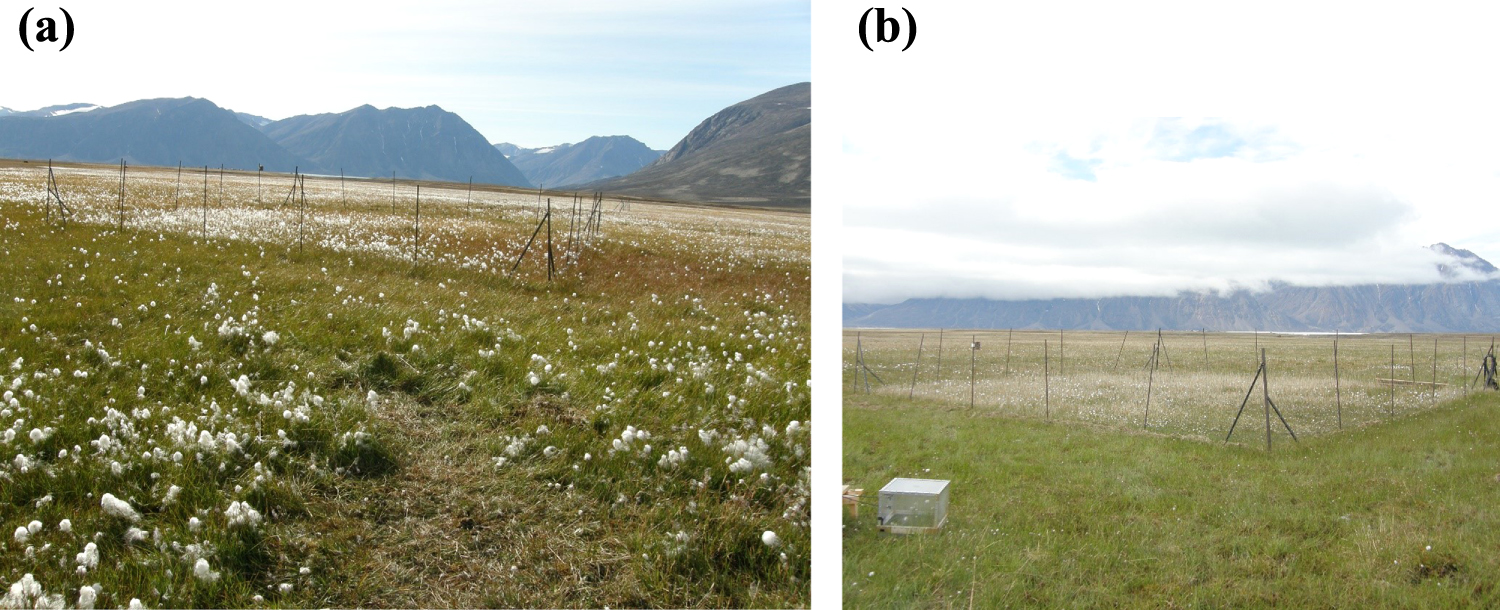
Strong relationships between NEE and the living plant biomass have been found in several previous studies (e.g. Ström and Christensen 2007, Sjögersten et al 2008). The relationship is generally attributed to a close link between photosynthetically active biomass and ecosystem carbon uptake. A majority of studies have found that the net ecosystem uptake of CO2 (NEE) decreases with higher grazing pressure (e.g. Sjögersten et al 2011, Cahoon et al 2012, Falk et al 2014, Vaisanen et al 2014). In contrast we found a significant decrease in NEE three years after herbivore exclusion and in GPP already after two years (table 4). The rapid response in GPP following removal of grazing may be explained by the decrease in density of tillers in EX areas (tables 2 and 3), as tiller density is a major determinant of NEE. Very few studies have looked at how herbivory in arctic mires feeds back on the ecosystem carbon balance. The difference between our findings and others is likely explained by differences in ecosystem type, grazing pressure, time scale and/or grazer community studied.
We found a large inter-annual difference in the magnitude of the mean CO2 fluxes (table 4). The study was, however, only conducted over three years and it is not possible to draw any certain conclusions as to what primarily controls this variation. It can, however, be speculated that the inter-annual differences in NEE are largely due to variations in plant productivity as a result of different climatic conditions between the years. NEE was particularly low in 2013, which was very dry and cold compared to 2011 and 2012. These conditions will most likely lead to a reduction in plant growth and productivity. Offering some support for this argument, the number of tillers was significantly lower in 2013 than in 2011 (table 2). The dry conditions in 2013 may in contrast increase Reco since aerobic decomposition rates increase (Oberbauer et al 1992), which may offer some explanation to the generally higher Reco values in 2013 (table 4). Irrespective of the inter-annual variations, both C and EX areas had a negative NEE and acted as C-sinks in all years, although the magnitude of this sink varied between years and treatment. Three years into the experiment it was obvious that removal of grazing decreased the C-sink function of the ecosystem, as the mean CO2 uptake in EX was almost half of that in grazed areas (table 4).
Very few studies have to date focused on the effect of herbivory on CH4 fluxes in wet high arctic habitats (Sjögersten et al 2011, Falk et al 2014) and the findings from these studies contrasts with our finding of a 44% lower CH4 emission in EX than in C areas following three years of exclusion. In a study on Svalbard, Sjögersten et al (2011) reported no changes in the CH4 fluxes between grazed and un-grazed plots after 4 years of exclusion of geese. However, the CH4 fluxes reported in this study were very low and the different grazing pattern of grubbing geese may not make this ecosystem and its responses fully comparable with our study. In a recent study in the same Zackenberg mire we found lower CH4 emission in plots clipped to simulate increased grazing (Falk et al 2014), which as for NEE, showed that there is a clear difference in the ecosystem response to changes in grazing pressure alone, and to the actual removal of the grazers (i.e. excluding both grazing and trampling etc).
High plant productivity, i.e. GPP and NEE, have been found to stimulate CH4 emission in several studies (e.g. Joabsson and Christensen 2001, Ström and Christensen 2007, Lai et al 2014). Consequently, it is very likely that the lower CH4 flux in EX compared to C areas in 2013 is related to lower GPP and NEE in these areas and as a consequence a lower substrate availability for CH4 production. Also supporting this is the low number of Eriophorum tillers in the EX (table 4). We have previously shown that there is a clear linkage between CH4 flux, the number of Eriophorum tillers and the amount of labile substrate for CH4 production in the Zackenberg mire (Ström et al 2012, Falk et al 2014) with higher Eriophorum coverage leading to higher substrate availability and CH4 flux. Studies from other ecosystems (or performed in laboratory) confirm the importance of Eriophorum species for methane emissions (e.g. Greenup et al 2000, Joabsson and Christensen 2001, Ström et al 2003, Ström and Christensen 2007) and substrate availability (acetic acid) in pore water (Ström et al 2003, 2005, Ström and Christensen 2007). Additional and possibly additive explanations to the lower CH4 flux in EX than in C areas in 2013 may be the lower tiller number, lower Ts and higher WtD in EX this year (table 4). As both WtD and vascular transport of CH4 from anoxic peat depth to the atmosphere may affect the rate of methane oxidation in oxic peat layers (e.g. Bellisario et al 1999, Greenup et al 2000) and CH4 flux and production can increase with Ts (e.g. Tagesson et al 2013).
It may be speculated that the lower Ts in EX compared to C in 2013 was due to the thicker moss-layer. Van der Wal et al (2001) and Van der Wal and Brooker (2004) found a temperature decrease in the same order of magnitude as the one in our study in response to decreased grazing and attributed this increase to moss being an effective heat insulator with its low thermal conductance. In addition, shading by the standing litter (Henry 1998) may together with the higher reflection of dry litter (Lorenzen and Jensen 1988) contribute to further cooling of the soil. The results for Ts in our study was, however, ambiguous since it was significantly lower in EX than in C in 2011 and 2013, while in 2012 it was significantly higher in EX (table 4). Similarly, for the relationship between AL and Ts: in 2013 the lower Ts in EX areas seemed to significantly affect AL. This relationship was, however, not validated either in 2011 or 2012. Consequently, these relationships need further attention before any valid conclusions can be drawn.
A complicating factor that to some extent affects our ability to draw fully clear conclusions regarding the effect of muskoxen exclusion from the results of this study is that we in 2013 also found significant differences between C and SC areas in several variables, similar to what was found for EX, however, less pronounced (figure 1 and table 4). As previously, stated WtD and Ts may affect CH4 flux, as might vegetation composition and structure. Winter precipitation and snow-cover have large effects on the hydrological regime of the landscape (Zimov et al 1996, Fahnestock et al 1999), with more snow leading to decreased oxygen availability and an increase in the CH4 flux. In contrast, more snow may decrease the length of the growing season and the productivity of the ecosystem possibly having negative effects on the CH4 flux. In early spring 2012, two years after the installation of the exclosures, we measured the snow depth in all treatments, and found no significant effects of the fences (Schmidt, unpublished results). Christiansen (2001) found that snow-depth in Zackenberg often exceeded 1 m, consequently, the depth would in general exceed the height of the fences used in this study. We also find it rather unlikely that the large mesh size (10 × 10 cm) of the fences should substantially affect the snow depth. An alternative explanation for the differences between C and SC may be found in the foraging behavior of muskoxen around the fences as significant higher biomass of mosses (figure 1) indicates that muskoxen are grazing and trampling less in these areas. The effect of the snow fences in this experimental set-up however requires further studies in order for it to be fully evaluated.
In conclusion, this study shows that a change in the abundance of muskoxen at Zackenberg may rapidly alter the structure and vegetation composition, and ultimately affect the carbon balance. Based on previous experiments (Falk et al 2014) we hypothesized that exclusion of grazing would lead to an increase in the number of vascular plant tillers, which in turn would lead to an increase in NEE, GPP and CH4 emission. These hypotheses were not supported by the findings of this study and instead we found the opposite, with a decrease in tiller number, NEE and CH4 emission. We believe that the most likely reason for these opposing findings were the observed changes in vegetation structure. Factors such as a more developed moss-layer found in exclosures that resulted in decreased tiller formation and hereby a lower CO2 uptake seemed to exert a stronger disturbance compared to grazing alone. Although, both grazed and ungrazed areas acted as CO2 sinks during the growing season, the sink function decreases substantially in ungrazed plots. The removal of grazing in addition decreased the CH4 flux, presumably due to lower substrate availability for CH4 production as a result of a decrease in the productivity and abundance of Eriophorum in ungrazed areas. Further studies are however needed to fully understand the C-balance of these ecosystems and the intricate interactions between herbivores and ecosystem development in these regions.
Acknowledgments
The exclosure experiment was funded by the Danish Environmental Protection Agency, and established in close collaboration with Mads C Forchhammer, who thus made this project possible. The study was carried out as part of the strategic research program: Biodiversity and Ecosystem services in a Changing Climate (BECC), Lund University and the Lund University Center for Studies of Carbon Cycle and Climate Interactions (LUCCI). The study was also supported by the Nordic Center of Excellence, DEFROST, and the EU PAGE21 project. The research was financed by BECC and INTERACT (International Network for Terrestrial Research and Monitoring in the Arctic). We are also grateful to Aarhus University, Denmark and personnel at Zackenberg field station for logistical support and to Caroline Jonsson and Ulrika Belsing for field assistance in 2012 and 2013.