

Abstract
We reconstruct the evolution of ocean acidification in the California Current System (CalCS) from 1979 through 2012 using hindcast simulations with an eddy-resolving ocean biogeochemical model forced with observation-based variations of wind and fluxes of heat and freshwater. We find that domain-wide pH and  in the top 60 m of the water column decreased significantly over these three decades by about −0.02 decade−1 and −0.12 decade−1, respectively. In the nearshore areas of northern California and Oregon, ocean acidification is reconstructed to have progressed much more rapidly, with rates up to 30% higher than the domain-wide trends. Furthermore, ocean acidification penetrated substantially into the thermocline, causing a significant domain-wide shoaling of the aragonite saturation depth of on average −33 m decade−1 and up to −50 m decade−1 in the nearshore area of northern California. This resulted in a coast-wide increase in nearly undersaturated waters and the appearance of waters with
  , leading to a substantial reduction of habitat suitability.
Averaged over the whole domain, the main driver of these trends is the oceanic uptake of anthropogenic CO2 from the atmosphere. However, recent changes in the climatic forcing have substantially modulated these trends regionally. This is particularly evident in the nearshore regions, where the total trends in pH are up to 50% larger and trends in  and in the aragonite saturation depth are even twice to three times larger than the purely atmospheric CO2-driven trends. This modulation in the nearshore regions is a result of the recent marked increase in alongshore wind stress, which brought elevated levels of dissolved inorganic carbon to the surface via upwelling. Our results demonstrate that changes in the climatic forcing need to be taken into consideration in future projections of the progression of ocean acidification in coastal upwelling regions.
Export citation and abstract BibTeX RIS

Original content from this work may be used under the terms of the Creative Commons Attribution 3.0 licence. Any further distribution of this work must maintain attribution to the author(s) and the title of the work, journal citation and DOI.
1. Introduction
The primary driver for the large-scale acidification of the world's oceans is the increase in anthropogenic CO2 in the atmosphere, caused by the burning of fossil fuels and land use change (e.g., Orr et al 2005, Doney et al 2009, Rhein et al 2013). The resulting disequilibrium in CO2 across the air–sea interface forces anthropogenic CO2 into the ocean, causing a global increase in the dissolved CO2 concentration, and also a decrease in pH and in the saturation state, Ω, with regard to calcium carbonate (CaCO3) minerals (e.g., Feely et al 2004, Orr et al 2005, Zeebe 2012). Yet, it is well recognized that local changes in ocean circulation and ocean biology, or other processes, such as river input (e.g., Cai et al 2011, Breitburg et al 2015) or atmospheric deposition (e.g., Doney et al 2007) can substantially modulate the evolution of oceanic pH and Ω. Especially in coastal systems ocean acidification may progress rather differently than in the open ocean. This is due in part to their proximity to land (e.g., Duarte et al 2013) but also owing to the high potential in coastal systems for local changes in circulation and biology to impact the ocean's carbonate system (e.g., Turi et al 2014). Eastern boundary upwelling systems (EBUS) may be particularly prone to such modifications of atmospheric CO2-driven ocean acidification, because of the key role of the coastal upwelling process, which makes these systems naturally low in pH and Ω. Thus, relatively small changes in the intensity of upwelling in these systems may cause substantial changes in the rate of progression of ocean acidification (e.g., Feely et al 2008, Hauri et al 2009, Gruber 2011, Hofmann et al 2011, Gruber et al 2012, Alin et al 2012, Harris et al 2013, Rhein et al 2013, Bates et al 2014, Lachkar 2014, Williams et al 2015).
Recent studies suggest that alongshore, upwelling-favorable wind stress has increased in nearly all of the EBUS (Sydeman et al 2014), including the California Current System (CalCS; e.g., Bakun 1990, Schwing and Mendelssohn 1997, Mendelssohn and Schwing 2002, Demarcq 2009, García-Reyes and Largier 2010, Narayan et al 2010, Seo et al 2012). This is consistent with the hypothesis by Bakun (1990) that the strengthening of the thermal land–sea gradient driven by global surface warming will cause stronger equatorward winds along the western coasts of the continents. This hypothesis also implies that the intensification of upwelling may persist as the planet continues to warm (e.g., Snyder et al 2003, Diffenbaugh et al 2004, Wang et al 2015).
So far, any relevant observations of ocean acidification parameters in EBUS are primarily limited to the  century (Borges et al 2009), which makes it challenging to investigate how these changes in upwelling-favorable winds might have altered the progression of ocean acidification over decadal time scales. In fact, the degree to which EBUS, and particularly the CalCS, are prone to ocean acidification has emerged clearly only in the last decade (e.g., Feely et al 2008, 2009, Wootton et al 2008, Hauri et al 2009, Gruber et al 2012, Hauri et al 2013a, 2013b, Leinweber and Gruber 2013, Bednaršek et al 2014). For instance, Feely et al (2008) observed waters undersaturated with respect to aragonite, the least stable mineral form of CaCO3, within the top 20–40 m of the water column in some CalCS coastal regions. Bednaršek et al (2014) reported that within the top 100 m up to 70%–90% of the total water volume was undersaturated in widespread areas along the coast, causing measurable shell dissolution in the pteropod Limacina helicina. Although coastal upwelling regions such as the CalCS tend to be accustomed to extreme fluctuations in pH and Ω due to the seasonality and episodicity of wind-driven upwelling (e.g., Hauri et al 2009, Juranek et al 2009, Hofmann et al 2011, Frieder et al 2012, Harris et al 2013, Leinweber and Gruber 2013), it is very likely that these regions will become exposed to more frequent, prolonged and intense events of this nature in the near future (Gruber et al 2012, Hauri et al 2013a, 2013b). Moreover, an acceleration of ocean acidification reduces the time that calcifying organisms have to adapt to such changes and can therefore pose an increased risk to local ecosystem services (e.g., Soto 2002, Barton et al 2012, 2015, Waldbusser et al 2014, 2015, Waldbusser and Salisbury 2014, Bednaršek and Ohman 2015).
Given the lack of long-term observations documenting the progression of ocean acidification over the last few decades, hindcast model simulations forced with observation-based estimates of variations in winds and the fluxes of heat and freshwater are one of the few means to reconstruct this history (see, e.g., Lenton et al (2015), for an empirical model-based approach). We follow this model-based approach and employ a coupled physical-biogeochemical model on the basis of the Regional Oceanic Modeling System (ROMS), configured for the CalCS at eddy-permitting resolution. Our objectives are (i) to investigate the progression of ocean acidification in the CalCS over the period from 1979 to 2012, i.e., over the period when atmospheric CO2 increased from about 335 μatm to 394 μatm, and (ii) to separate the effect of the rise in atmospheric CO2 from the effect of changes in the climatic forcing. We do not take into consideration other processes that potentially affect ocean acidification, such as changes in deposition by rivers and through the atmosphere, as we assume these effects to be of minor importance in this region.
2. Model and methods
We use an eddy-resolving coupled physical-biogeochemical ocean model to simulate the evolution of ocean acidification in the CalCS from 1979 to 2012. The physical model is based on the UCLA-ETH version of ROMS (Marchesiello et al 2003, Shchepetkin and McWilliams 2005). Coupled to the physical model is a nitrogen-based nutrient-phytoplankton-zooplankton-detritus model (Gruber et al 2006) that was extended with a carbon module (Gruber et al 2012, Hauri et al 2013b, Turi et al 2014). The CalCS model setup employed here has a resolution of 5 km, and extends roughly from 30°N to 50°N along the US West Coast and about 1250 km westward into the open Pacific. This grid setup and these parameters correspond exactly to those used by Turi et al (2014). While previous simulations with similar setups using ROMS were climatologically forced (Gruber 2011, Hauri et al 2013b, Turi et al 2014), we focus here on the impact of variations and trends in the atmospheric forcing.
We ran two hindcast simulations ('HCast') with variable atmospheric forcing and lateral boundary conditions, with the two runs differing only in the applied wind stress forcing and their length of simulation. For both HCast simulations, we used daily fluxes of heat and freshwater from ECMWF's ERA-Interim reanalysis (Dee et al 2011). Atmospheric CO2 was prescribed to follow the observed atmospheric trend (Cooperative Global Atmospheric Data Integration Project 2013). We forced the model at the lateral boundaries with a combination of climatological fields based on observations and time-varying anomaly fields derived from a global hindcast simulation with the NCAR CCSM3 model (Graven et al 2012).
In the first hindcast simulation ('HCast-ERAI'), we used the daily wind stress forcing from ERA-Interim as well. However, as ERA-Interim has a relatively coarse resolution of ∼79 km, we ran a second hindcast simulation ('HCast-CCMP') where we forced the model with daily wind stress computed from the wind speed data of NASA's CCMP reanalysis dataset (Atlas et al 2011). This latter forcing has a horizontal resolution of 0.25°, and therefore may be better suited to capture the response of coastal upwelling to recent climate change (e.g., Jacox et al 2014, Renault et al 2015). As CCMP provides only wind speed, we calculated wind stress using the drag coefficient formulation after Hersbach (2011). Due to differing data availability, the HCast-ERAI simulation was run for the entire analysis period, i.e., 1979–2012, whereas the HCast-CCMP simulation only spans the period from 1988 to 2011.
For both HCast simulations, the model was spun up for 10 years starting from observations and using so-called 'normal-year forcing', i.e., climatological monthly forcing with added daily variations from a particular year. The spinup for the HCast-ERAI simulation used the normal-year forcing from ERA-interim and began in the year 1969 with daily anomalies from 1985, while the spinup for the HCast-CCMP simulation was initialized in 1978 and was forced with the normal year forcing from CCMP from 1991. More details on the model's atmospheric forcing and the lateral boundary conditions are given in the appendix.
The appendix also contains a detailed model assessment section, in which we demonstrate that both forcing products are able to reproduce the observed cooling over the last few decades (e.g., García-Reyes and Largier 2010, Seo et al 2012), as well as the accompanying increase in near-surface chlorophyll since the late 1990s (e.g., Kahru et al 2009, 2012). In addition, this setup, forced with a different set of atmospheric boundary conditions than used previously, performs on average as well as previous setups with regard to long-term mean sea surface temperature (SST) and chlorophyll (not shown; Gruber 2011, Hauri et al 2013b, Turi et al 2014). The two forcing products have complimentary strengths and weaknesses, with HCast-CCMP better capturing the trends in SST, while HCast-ERAI is better in simulating the alongshore increase in chlorophyll.
To separate out the effect of recent changes in the climatic forcing on ocean acidification, we additionally ran two 'constant climate' ('CClim') simulations under both forcing products ('CClim-ERAI' and 'CClim-CCMP'). In these simulations, only atmospheric CO2 and lateral dissolved inorganic carbon (DIC) were allowed to increase, while the other surface and lateral boundary conditions are climatological reflecting a normal year, i.e., the same boundary conditions we had used for the spinup. Assuming that the trends from the HCast and CClim simulations are linearly additive, we use the difference between these two simulations to identify the contribution of variable climatic forcing, without the effect of increasing atmospheric CO2 (i.e., HCast-CClim). We decided to use this approach of linear partitioning instead of directly computing trends from a 'climate only' simulation in order to remove any model internal variability that is unrelated to changes in the climatic forcing. By comparing our trend results to trends from the 'climate-only' simulation and finding only minimal differences in absolute trend values and domain-wide patterns, we determined that in our case this approach is valid (not shown).
The full suite of carbonate chemistry parameters was calculated offline from the modeled state variables temperature, salinity, nitrate, DIC and alkalinity (Alk) using the carbonate chemistry routines from the ocean carbon-cycle model intercomparison project (Orr et al 2000). We calculate all trends by least squares linear regressions, using the p-value from a Student's t-test for the statistical significance, accounting for autocorrelation by reducing the degrees of freedom according to the equivalent sample size (after Zwiers and von Storch 1995).
3. Evolution of ocean acidification
Over the whole model domain and over the period 1979/1988 to 2012, we model in the HCast simulations a decrease in surface pH and  in the top 60 m of the water column of −0.020 ± 0.002 dec−1 and −0.12 ± 0.02 dec−1, respectively (averaged over both HCast simulations with the uncertainty representing the spatial variability; figures 1(a), (b), (d) and (e) and table 1). These CalCS domain-wide trends in ocean acidification correspond roughly to those observed globally and in particular for the North Pacific (see table 6 in Williams et al 2015). Lauvset et al (2015) estimated a global surface pH trend of −0.018 ± 0.004 dec−1 for the period 1991–2011, which is statistically indistinguishable from our result for the whole CalCS domain (table 1). In particular, for the Hawaii Ocean Time (HOT) series at Station ALOHA and for the time period 1988–2014, Bates et al (2014) found decreases in pH and
  of −0.016 ± 0.001 dec−1 and −0.084 ± 0.011 dec−1, respectively. The IPCC's Fifth Assessment Report (Rhein et al 2013) confirms these trends for HOT and offers a further estimate for the pH decline in the North Pacific of −0.017 dec−1, based on two hydrographic lines along 152°W in 1991 and 2006 (Byrne et al 2010). Furthermore, Fay and McKinley (2013) established that surface ocean pCO2 trends in the north Pacific from 1981 to 2010 were comparable to the increase in atmospheric pCO2 over the same time period (roughly 17 μatm dec−1; black line in figure 2(b)). This trend is very close to our modeled pCO2 trend for the CalCS of 18.8 ± 3.5 μatm dec−1 (table 1).

Figure 1. Trends per decade in pH,  and
and  from (a)–(c) the HCast-ERAI simulation (1979–2012) and (d)–(f) the HCast-CCMP simulation (1988–2011). pH and
  trends were averaged over the top 60 m of the water column. Negative trends in
  denote a shoaling. All trends are significant at the 95% level.
Download figure:
Standard image High-resolution image
Figure 2. (a) Model analysis domain, indicating three regions of interest and highlighting the most prominent geographical features. The latitudinal extent of Regions 1 and 2 covers the coastal area roughly from the USA/Mexico border (∼33°N) to just south of the Columbia river mouth (∼46°N). Temporal evolutions from 1979 to 2012 of annual mean (b) pCO2, (c) pH, (d)  and (e)
  from the HCast-ERAI (solid lines) HCast-CCMP (dashed lines) simulations, averaged over the three regions shown in panel (a) (color-coded). The black line in panel (b) indicates the temporal evolution of the model's atmospheric CO2 forcing. pCO2, pH and
  trends were averaged over the top 60 m of the water column.
Download figure:
Standard image High-resolution imageTable 1.
Trends per decade in pCO2, pH,  and
and  from the HCast and CClim simulations under ERA-Interim and under CCMP forcing. The 'climatic modulation' is defined as (HCast-CClim)/CClim. Trends were averaged over the whole model analysis domain ('total'; sum of R1–R3; figure 2(a)) and over the three regions R1–R3 separately and are all significant at the 95% level. Negative trends in
  denote a shoaling. pCO2, pH,
  were averaged over the top 60 m of the water column. The uncertainty in the trends represents the spatial variability, i.e., standard deviation, over the respective regions.
| ERA-Interim | CCMP | ||||||
|---|---|---|---|---|---|---|---|
| Variable | Regiona | HCast | CClim | Climatic modulation (%) | HCast | CClim | Climatic modulation (%) |
| pCO2 (μatm dec−1) | Total | 17.9 ± 3.1 | 17.7 ± 2.9 | 1.1 | 19.6 ± 3.9 | 17.1 ± 2.0 | 14.6 |
| R1 | 25.8 ± 3.6 | 17.9 ± 3.5 | 44.1 | 28.9 ± 3.3 | 18.4 ± 2.2 | 57.1 | |
| R2 | 20.6 ± 2.7 | 25.5 ± 2.6 | −19.2 | 24.2 ± 2.9 | 17.6 ± 1.8 | 37.5 | |
| R3 | 17.0 ± 1.8 | 17.2 ± 2.1 | −1.2 | 18.5 ± 2.3 | 17.0 ± 2.0 | 8.8 | |
| pH (dec−1) | Total | −0.018 ± 0.002 | −0.017 ± 0.002 | 5.9 | −0.021 ± 0.003 | −0.017 ± 0.002 | 23.5 |
| R1 | −0.024 ± 0.002 | −0.016 ± 0.002 | 50.0 | −0.029 ± 0.003 | −0.017 ± 0.002 | 70.6 | |
| R2 | −0.019 ± 0.002 | −0.020 ± 0.002 | −5.0 | −0.024 ± 0.003 | −0.016 ± 0.002 | 50.0 | |
| R3 | −0.018 ± 0.001 | −0.017 ± 0.002 | 5.9 | −0.020 ± 0.002 | −0.017 ± 0.002 | 17.6 | |
1 cm (dec−1) (dec−1) |
Total | −0.11 ± 0.01 | −0.07 ± 0.01 | 45.8 | −0.13 ± 0.02 | −0.07 ± 0.01 | 87.1 |
| R1 | −0.11 ± 0.01 | −0.06 ± 0.01 | 91.1 | −0.14 ± 0.02 | −0.06 ± 0.01 | 130.5 | |
| R2 | −0.09 ± 0.01 | −0.07 ± 0.01 | 19.2 | −0.13 ± 0.01 | −0.06 ± 0.01 | 120.3 | |
| R3 | −0.11 ± 0.01 | −0.07 ± 0.01 | 45.2 | −0.13 ± 0.02 | −0.07 ± 0.01 | 84.5 | |
 (m dec−1) (m dec−1) |
Total | −28.4 ± 6.1 | −14.3 ± 3.4 | 98.6 | −38.2 ± 6.5 | −12.7 ± 3.9 | 200.8 |
| R1 | −36.3 ± 3.4 | −16.6 ± 3.7 | 118.7 | −46.6 ± 4.5 | −15.9 ± 4.4 | 193.1 | |
| R2 | −23.5 ± 6.0 | −15.7 ± 2.7 | 49.7 | −33.7 ± 6.7 | −11.1 ± 2.2 | 203.6 | |
| R3 | −28.1 ± 5.8 | −14.1 ± 3.3 | 99.3 | −37.8 ± 6.1 | −12.5 ± 3.8 | 202.4 | |
aThe surface areas of R1–R3 are 98 650 km2, 69 785 km2 and 1313 341 km2, respectively. The total surface area amounts to 1481 776 km2.
The ocean acidification signal penetrates deeply into the thermocline of the CalCS, causing a significant domain-wide shoaling of the aragonite saturation depth
( i.e., the depth below which
  ) by an average rate of −33 ± 6 m dec−1 (figures 1(c) and (f)). The strongest upward migration of
  occurred in the northern nearshore regions around Cape Mendocino (∼40°N), with regional values of more than 50 m dec−1. This result is comparable to the
  trend of 50 m dec−1 inferred by Feely et al (2012) from two repeat hydrography sections measured in 1994 and 2004 along a transect line crossing through the CalCS. These changes occur at a mean depth of around −200 m in the model, which is somewhat shallower than the observed depth (Feely et al 2008, Gruber et al 2012). Nonetheless, both modeled and measured results indicate that this shoaling is likely responsible for the substantial compression of habitat suitability for organisms sensitive to ocean acidification across the entire CalCS (e.g., Feely et al 2008, Bednaršek et al 2014, Bednaršek and Ohman 2015).

Figure 3. Temporal evolution of monthly mean volume fraction of water with a specific  in the nearshore 100 km (i.e., averaged over regions 1 and 2; figure 2(a)). Panels (a) and (b) show results from the HCast-ERAI simulation for the top 60 m and the 60–120 m layer of the water column, respectively. Panels (c) and (d) show results from the HCast-CCMP simulation for the same layers, respectively.
Download figure:
Standard image High-resolution image
Figure 4. Trends per decade in pH,  and
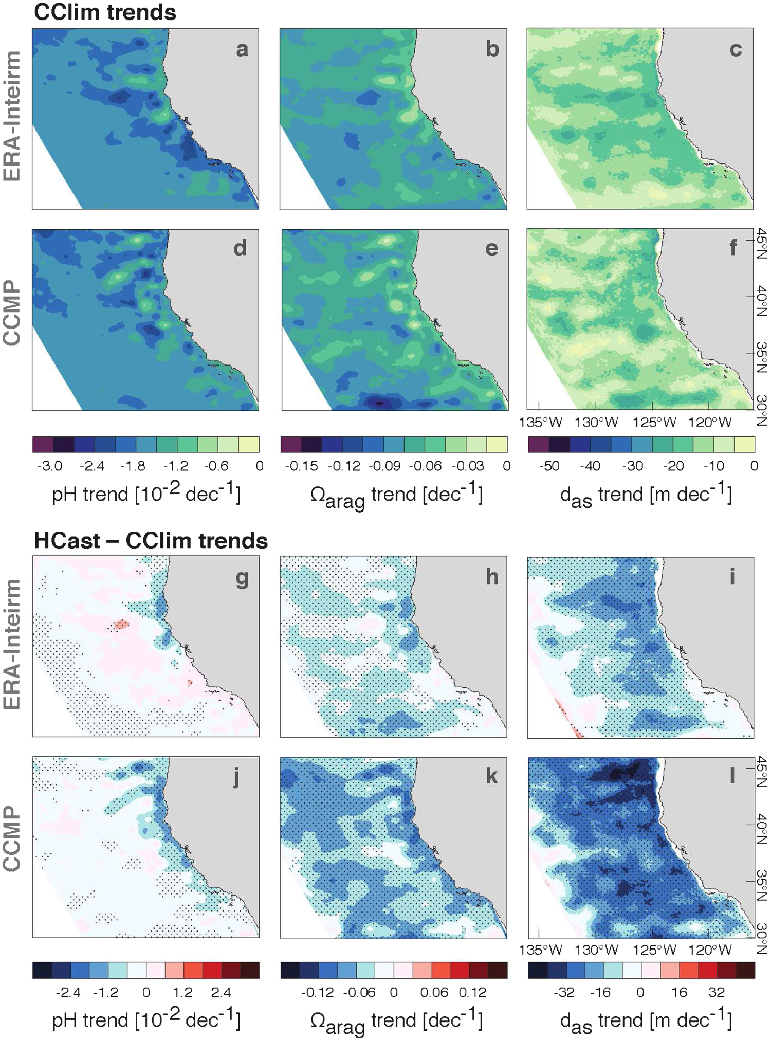
and  from (a)–(c) the CClim-ERAI simulation, (d)–(f) the CClim-CCMP simulation, (g)–(i) the difference HCast-ERAI-CClim-ERAI and (j)–(l) the difference HCast-CCMP-CClim-CCMP. Note that the color bar ranges in (a)–(f) match those in figure 1 to be directly comparable. pH and
  trends were averaged over the top 60 m of the water column. Negative trends in
  denote a shoaling. Trends in (a)–(f) are significant at the 95% level. The black stippling in (g)–(l) denotes trends significant at the 95% level and higher.
Download figure:
Standard image High-resolution image
Figure 5. Decomposition of trends in (a) pCO2, (b) pH and (c)  into four components representing the contributions of trends in DIC, Alk, temperature (T) and salinity (S). The total trends (leftmost panels) were calculated from the difference HCast-CClim under ERA-Interim forcing and thus represent trends due to changes in the climatic forcing.
Download figure:
Standard image High-resolution imageSubstantial regional differences exist in the trends across the CalCS. In particular, we find much stronger trends in the nearshore areas, although to different degrees in the two simulations. In the HCast-ERAI simulation, the region of largest trends is located between San Francisco Bay, California, and Cape Blanco, Oregon (∼38–43°N; figures 1(a)–(c)), whereas in the HCast-CCMP simulation, the region of strongest increase extends further to the north and to the south (∼35–45°N; figures 1(d)–(f); see figure 2(a) for geographical locations). In these areas, we have reconstructed maximum decreases in pH and  of up to −0.03 dec−1 and −0.15 dec−1, respectively, and a maximum shoaling of
  of up to −40 to −50 m dec−1. In contrast to the trends in pH, which show a strong cross-shore gradient, the regions of strongest trends in
  and
and  extend up to 500–600 km offshore.
To quantify these trends in more detail, we focus our analysis on three regions within our model domain (figure 2(a)). In both HCast simulations, the largest trends occur in the northern coastal region (R1), where pCO2 trends are on average 5 μatm dec−1 larger than in the southern coastal region (R2; figure 2(b)). Similarly, pH and  decrease by about −0.005 dec−1 and −0.01 dec−1 more, and
  shoals by about −13 m dec−1 more in R1 compared to R2 (figures 2(c)–(e)). Trends in the offshore region (R3) are the smallest for all three variables in both HCast simulations.
The HCast-CCMP simulation consistently exhibits larger domain-wide and regional trends in pCO2, pH,  and
and  than the HCast-ERAI simulation (table 1). This can partly be explained by the larger alongshore wind stress trends in CCMP compared to ERA-Interim (figure 6(c)), especially in the nearshore 100 km. This could have a more offshore-reaching effect on ocean acidification due to the anomalous upwelling and subsequent offshore transport of waters high in DIC and low in pH and carbonate ion concentrations ([CO
 ]), which could explain why the trends in pCO2, pH,
  are larger in the HCast-CCMP simulation in the offshore region as well.

Figure 6. (a) Temporal evolution of the monthly PDO index from 1979 to 2012 with the ±1 standard deviation thresholds indicated by black dashed lines. (b) Composite analysis of ERA-Interim and CCMP alongshore wind stress ( ) anomalies.
  anomalies were computed as anomalies of extreme negative years minus anomalies of extreme positive years and indicate the change over the whole time period (1979–2012 for ERA-Interim and 1988–2011 for CCMP). The original
  time series were first detrended and the annual cycle was removed. An extreme positive (negative) year is flagged if three or more months in that year exceed +1 std. (fall below −1 std.). (c) Total
  trends for ERA-Interim (1979–2012) and CCMP (1988–2011).
Download figure:
Standard image High-resolution imageA comparison of the temporal progressions of these four variables from the HCast-ERAI and HCast-CCMP simulations reveals that throughout the HCast-CCMP simulation from 1988 to 2011, pCO2 is lower, pH and  are higher and
  is deeper compared to the HCast-ERAI simulation (figures 2(b)–(e)). Although both simulations were spun up analogously, the initial conditions for the HCast-CCMP simulations in 1988 differ from the conditions for the same year during the HCast-ERAI simulation. This discrepancy could partly explain the difference in the absolute values and trends (see methods and appendix for a more detailed description of the spinup processes).
As a result of the more rapid evolution of ocean acidification in the nearshore 100 km, the compression of habitat suitability is even more acute there in comparison to the trends across the whole domain. A more detailed quantification of the distribution of the volumes of water within a particular  range in the nearshore 100 km and within the euphotic zone (0–60 m; averaged over R1 and R2) reveals that the volume of water with
  decreased by a factor of more than two under both forcings, becoming progressively rarer (figures 3(a) and (b)). While the volume of water with
  between 1.5 and 2.0 changed little, waters on the verge of undersaturation, i.e., waters with
  , became much more abundant, increasing in their volume from around 10% to over 30% of the total water mass.
In the upper aphotic zone, i.e., in the layer between 60–120 m, we model in both HCast simulations a decrease of waters with  to the point of disappearance by 2012 (figures 3(c) and (d)). The volume of nearly undersaturated water (
 ) increases in both HCast simulations, to occupy on an annual mean up to roughly 90% (ERA-Interim) and 80% (CCMP) of the total water mass in this layer. Furthermore, toward the end of both simulations, undersaturated waters (
 ) start to occur on a monthly basis, occupying up to 10% of the water mass.
Strong variations in the volumes of saturated and undersaturated waters are visible for both layers of the water column on seasonal and interannual time scales. The magnitudes of both seasonal and interannual variability in the volume of nearly undersaturated water ( ) are roughly equal and range between ± 5% and ± 15%. The interannual fluctuations largely reflect the impact of changes in the upwelling of waters with low saturation states, mostly associated with the appearance of El Niño/La Niña conditions (e.g., Frischknecht et al 2015, Jacox et al 2015).
Our reconstructed evolution of ocean acidification in the CalCS reveals that substantial changes have occurred in the last few decades and highlights that recent distributions of pCO2, pH, and  are very different from those that characterized the system a few decades ago. These reconstructions will put other observations of changes in biogeochemistry and ecosystems into historical context and provide a basis against which future projected changes can be compared to. Gruber et al (2012) demonstrated for example that the volume of undersaturated water that began to appear in the nearshore area between 60 and 120 m will become the norm by 2030. They also projected the appearance of undersaturated conditions in the top 60 m within the next decade. Furthermore, Hauri et al (2013a) suggested that it takes 20–30 years for trends in ocean acidification to emerge from the background variability in the CalCS. This finding is consistent with our trends in pCO2, pH,
  and
and  , which are highly significant across the whole domain (table 1) and thus are clearly distinguishable from the sub-decadal variability. Therefore, the fundamental alteration of habitat suitability for organisms and ecosystems vulnerable to ocean acidification has begun several decades ago, and is bound to become more accentuated in the coming decades.
4. Drivers of trends in ocean acidification
If the increase in atmospheric CO2 were the only driver for ocean acidification across the CalCS, one would expect a relatively uniform trend pattern. However, the substantial spatial variations in the ocean acidification trends seen in our reconstructed fields indicate a different picture. They suggest that local, yet climatically forced, processes must have modulated the purely atmospheric CO2-driven trends in the last few decades. This strong nearshore ocean acidification signal is due to a change in the upwelling of waters that are high in natural CO2, stemming from the remineralization of organic matter rather than an anthropogenic signal of the source waters from previous decades.
To quantify this climate variability-induced modulation in more detail, we compare the trends from the HCast simulations to the results from the corresponding CClim simulations, where we only allowed lateral DIC and atmospheric CO2 to vary. On average, the trends in pH,  and
and  in the CClim simulations exhibit much more homogeneous patterns of change compared to the results from the corresponding HCast simulations (figures 4(a)–(f)). Given the climatological forcing, the relatively small variability in the trends from the CClim simulations is a result of variations in the surface ocean buffer factor (Zeebe 2012) and also includes the effect of internally generated stochastic variability of the CalCS, reflecting its turbulent nature. The domain-wide changes in pH and
  are similar to those from the HCast simulations, i.e., average decreases of −0.017 ± 0.002 dec−1 and −0.07 ± 0.01 dec−1, respectively (averaged over CClim-ERAI and CClim-CCMP). The shoaling rate of
  of −13.5 ± 3.7 m dec−1, however, is only about half of that from the HCast simulation.
The modulating impact of the variable climatic forcing is substantial under both forcings and occurs primarily in the nearshore regions of the CalCS (figures 4(g)–(l)). Under ERA-Interim forcing, there is a division around San Francisco Bay (∼38°N) in the sign of the pH trends. In the northern nearshore region (R1), variations in the climatic forcing cause a more rapid decline in pH than solely through the rise in atmospheric CO2 (50% stronger decline, see table 1), whereas in the southern nearshore region (R2) these variations dampen the atmospheric CO2-driven trends, causing a slight increase in pH. This is also visible in the  and
and  trends, with a weaker decrease in
  and less shoaling of
  in R2 compared to R1. Under CCMP forcing, we model a more homogeneous climatic modulation of pH,
  and
and  within the nearshore 100 km, with magnitudes of on average 60%, 125% and 200%, respectively (see table 1 for the climatic modulations).
Thus, while it is unambiguous that recent climatic variations have impacted the trends in ocean acidification across most of the coastal CalCS in a substantial manner, the details of this modulation depend on the particular forcing applied to the model. Furthermore, while the pH trends are modulated primarily in the coastal regions, the impact of the climatic variations is stronger for the trends in  and
and  , and extends much further offshore. This also explains the fact that the domain-wide changes in
  and
and  differ substantially between the HCast and CClim simulations, while in the case of pH the domain-wide trends are nearly equal.
5. Climatic modulation of ocean acidification
To determine the processes responsible for the climatic modulation of the trends in ocean acidification, we employ a first-order Taylor expansion of the trends in the difference HCast-CClim averaged over the top 60 m of the water column for pCO2, pH and  . We expand the trends into components representing trends in DIC, Alk, temperature and salinity from the difference HCast-CClim (after Lovenduski et al 2007, Doney et al 2009, Turi et al 2014, see figure B3 for trends in DIC, Alk, temperature and salinity). This decomposition reveals that both under ERA-Interim and under CCMP forcing, the strong nearshore decline in pH is mainly driven by the local increase in DIC (figures 5(a) and B3(a) and (e)). The decrease in Alk and the surface cooling dampen the DIC effect to a certain extent, but are too weak to fully compensate (figures B3(b), (c), (f) and (g)). In the offshore regions, the positive effect of the decrease in Alk on pH is almost entirely balanced by the effect of the decreases in temperature and DIC. In the case of
  , the nearshore increase in DIC dominates the trends there, while the offshore decrease in Alk dominates the trends away from the coast, resulting in the almost domain-wide decrease in
  (figure 5(b)). In strong contrast to the trends in pH, the effect of the domain-wide cooling is negligible for the trend in
  . The contribution of trends in salinity is too small to significantly modify the trends in both pH and
  (figures B3(d) and (h)). In order to assess the role of biology in driving the modeled trends in the carbonate system, we computed the changes in the sources and sinks of [CO
 ]. Our results indicated no significant trends in the biologically driven changes in [CO
![${}_{3}^{2-}]$](https://content.cld.iop.org/journals/1748-9326/11/1/014007/revision1/erlaa1041ieqn77.gif) (not shown).
(not shown).
Thus, having eliminated changes in biology as an important contributor to our modeled trends, the coastal signature of the trends with nearshore high DIC and low temperatures clearly points to a change in upwelling as the dominant process underlying the climatic modulation of the ocean acidification trends. This is consistent with the alongshore wind stress trends in the forcing products (figure 6(c)). ERA-interim shows an increase in equatorward, upwelling-favorable wind stress to the north of roughly 38°N, whereas the trend is toward weaker equatorward wind stress to the south of this. CCMP alongshore wind stress trends are mostly positive, i.e., toward upwelling-favorable wind stress, all along the coast. This resulting pattern of increased upwelling in the northern subregion for ERA-Interim and of strong increases in upwelling along the entire coast for CCMP can explain our modeled pattern of ocean acidification due to the climatic modulation very well. This is consistent with findings from Turi et al (2014), who demonstrated that variations in DIC, driven by changes in circulation (i.e., upwelling), are the main driver for pCO2 variability in the nearshore 100 km of the CalCS.
The increased upwelling can also explain the much farther offshore reach of the climatic modulation for  and
and  relative to that of pH. This is because the stronger equatorward wind stress along the shores causes not only stronger upwelling, but also pulls the upper thermocline up, causing a shoaling of the isopycnals and the upward movement of the waters with undersaturated conditions. This thermocline shoaling extends to about 800 km offshore (not shown), explaining the wide reach of the stronger decline in
  and shoaling of
  .
.
With increased upwelling as the primary driver of the larger than expected trends, it befits us to demonstrate that these trends are reliable. A detailed comparison of the two wind products with mooring-based trend estimates (García-Reyes and Largier 2010) confirms the trends, with the CCMP wind stress data in general comparing more favorably to the in situ measurements (see appendix figures B1 and B2 ). Also the comparison of the modeled trends in SST and chlorophyll from both HCast simulations with satellite-based estimates supports our finding of substantial trends, again with the results from the HCast-CCMP simulation obtaining better agreements. However, the simulations under CCMP forcing only cover the period from 1988 to 2011 (24 years), whereas the ERA-interim simulations extend over 34 years. Thus, the latter simulations lend themselves better to the analyzes of multi-decadal trends, i.e., are less sensitive to the choice of beginning and end years.

Figure B1. Comparison of modeled versus satellite-observed trends per decade in (a) SST and (b) chlorophyll, based on monthly data. The leftmost and center panels show trends from the HCast-ERAI and HCast-CCMP simulations, respectively, while the rightmost panels show observed trends. Observed SST trends are based on monthly data from NOAA's AVHRR Pathfinder Version 5 SST Project (4 km horizontal resolution) spanning the period from June 1988 to December 2009 and observed chlorophyll trends are from the European Space Agency's GlobColour Project (0.25° horizontal resolution), with monthly values from September 1997 to December 2011, including observations from the Sea-viewing Wide Field-of-view Sensor (SeaWiFS), the Moderate Resolution Imaging Spectroradiometer on NASA Aqua Satellite (MODISA) and the Medium Resolution Imaging Instrument on ESA Envisat Satellite (MERIS). We sampled our model output over the same time periods to be directly comparable to the satellite observations. The black stippling denotes trends significant at the 95% level and higher.
Download figure:
Standard image High-resolution image
Figure B2. Comparison of trends per decade in (a) alongshore wind stress ( ) from ERA-Interim (red) and CCMP (orange) and (b) modeled SST forced with ERA-Interim and CCMP wind stress to trends in wind stress and SST measured at the 11 buoy stations (green). Trends are based on means over the upwelling season (March–July) and are given per decade for the common time period from 1988 to 2010. Positive
  trends denote equatorward wind direction. Trends which are significant at the 90% significance level and higher are indicated by the color-coded lines at the right side of each panel.
Download figure:
Standard image High-resolution imageAs pointed out previously by Chhak and Di Lorenzo (2007), the Pacific Decadal Oscillation (PDO), a leading mode of climate variability in the North Pacific region (e.g., Mantua and Hare 2002), has a significant effect on the depth of the upwelling cell in the CalCS. They found that during warm phases of the PDO, the upwelling cell is shallower, potentially limiting the supply of nutrients and DIC to the surface, whereas during cool phases, the opposite is the case. The PDO was predominantly in a warm phase at the beginning of our simulation (roughly 1979–1988; figure 6(a)), progressing to a cool phase toward the end of our simulation (roughly 2008–2012). A composite analysis of detrended annual mean alongshore wind stress with the PDO index highlights that during cool phases of the PDO, the nearshore 100 km of the CalCS experiences positive, equatorward wind stress anomalies of up to 0.02 N m−2 larger than during warm phases, both in the case of ERA-Interim and CCMP (figure 6(b)). As these anomalies are on the order of the total trends over the whole simulation (figure 6(c)), the observed transition from a warm to a cool phase of the PDO over this time period could serve as a possible explanation for the observed trend toward more upwelling-favorable alongshore wind stress. The study by Feely et al (2012) found a shoaling of the aragonite saturation depth in the CalCS to depths of around −150 m over a 10 year period between 1994 and 2004. Around the same depth they also found an increase in cool, CO2-rich waters, which was consistent with measurements by Di Lorenzo et al (2005), who found a cooling and freshening of waters in the southern CalCS, which they attributed to an increase in southward advection of waters with those properties. These results support our finding that a combination of physical and chemical properties affect the carbonate system of the CalCS and that local changes in circulation can contribute significantly to ocean acidification, in addition to the direct effect of rising atmospheric CO2.

Figure B3. Trends per decade in DIC, Alk, temperature (T) and salinity (S) from (a)–(d) the difference HCast-ERAI-CClim-ERAI and (e)–(h) the difference HCast-CCMP-CClim-CCMP.
Download figure:
Standard image High-resolution image
Without a proper attribution, however, it is not possible to determine whether these trends in the alongshore wind stress are primarily the result of unforced variations of the climate system related to the PDO and to other modes of climate variability, or whether they are indeed fingerprints of ongoing anthropogenic climate change, as has been alluded to by a number of studies in recent decades (e.g., Bakun 1990, Diffenbaugh et al 2004, Narayan et al 2010, Sydeman et al 2014, Wang et al 2015).
6. Summary and conclusions
We used two sets of simulations from an eddy-resolving ocean biogeochemical model of the CalCS forced with two different wind products to (i) reconstruct trends in ocean acidification from 1979 to 2012 and (ii) separate the effects of the recent increase in atmospheric CO2 and of changes in the climatic forcing on these trends. To this end, we compared a simulation with fully transient atmospheric forcing and lateral boundary conditions ('HCast') to a simulation where only atmospheric CO2 and lateral DIC were allowed to vary ('CClim').
Irrespective of the forcing product, our model reconstructs domain-wide decreases in surface ocean pH and  that correspond roughly to those seen in the global ocean. In addition, we model a rapid shoaling of the depth of the saturation horizon. Across the entire domain it is found to have moved upward at a rate of −28 to −38 m dec−1, leading to a rapid compression of the volume of waters that are supersaturated with regard to aragonite.
The most severe changes in ocean acidification occur in an area limited to the first 100 km along the coast. In the case of the HCast-ERAI simulation, this area is located roughly between San Francisco Bay and Cape Blanco, Oregon (∼38–43°N), whereas in the HCast-CCMP simulation the area of maximum trends is more widespread (∼35–45°N). In these areas, ocean acidification has been progressing at rates up to 30% faster than what is found for the whole domain. This caused a more rapid emergence of undersaturated waters with respect to aragonite than would have been expected on the basis of the trends in atmospheric CO2 alone. Furthermore, the upwelling of waters high in natural CO2 that has accumulated at depth over time, masks any anthropogenic signal of the source waters of the CalCS, which would carry a lower CO2 signal from decades prior to upwelling.
While there existed essentially no undersaturated waters with respect to aragonite ( ) in the upper aphotic zone (60–120 m) of the nearshore 100 km in the late 1970s, such water masses can now occupy up to 10% of the total water mass of this layer. These strong historical changes in the biogeochemical habitat are bound to have had an effect on organisms and ecosystems that are potentially vulnerable to ocean acidification. There exist only a handful of studies that have looked at longer-term changes in organisms and ecosystems and related them to ocean acidification (e.g., Ohman et al 2009, Mackas and Galbraith 2012, Bednaršek et al 2014, Bednaršek and Ohman 2015) and the records are generally sparse in space and time and are often confounded by additional impacts such as warming and changes in oceanic productivity (e.g., Breitburg et al 2015). However, our results suggest that the observation by Bednaršek et al (2014) of pteropods with significant signs of dissolution in the upper ocean of the northern coastal region is a recent phenomenon. Our reconstructed history of ocean acidification in the CalCS will hopefully help undertake more historical impact assessments.
While averaged over the entire domain, the main driver of the trends in ocean acidification is the invasion of anthropogenic CO2 from the atmosphere into the ocean, climatic fluctuations substantially modulated these trends regionally, particularly in the nearshore 100 km. Specifically, in the northern coastal subregion, the climatic modulation caused a 50% stronger increase in pCO2 and decrease in pH than expected only from the increase in atmospheric CO2. In the same region, the decrease in  and shoaling of the aragonite saturation depth due to changes in the climatic forcing were two to three times above the purely atmospheric CO2-driven trends. These modulations are largely driven by a strong nearshore DIC increase caused by a trend toward increased upwelling, which itself is possibly linked to a negative trend of the PDO. It remains to be determined whether these changes simply reflect 'natural', i.e., unforced fluctuations of the climate system or whether they are the first signs of anthropogenic climate change. If it is the latter, then one can expect ocean acidification to continue advancing more rapidly than expected in the nearshore areas of the CalCS. If the former is the case, such past periods of rapid acidification will be followed by periods of moderate increase.
This modeling study is the first to investigate separately the effects of increasing atmospheric CO2 and of changes in the climatic forcing on ocean acidification in the CalCS. Our model results show a clear connection between a local increase in upwelling-favorable wind stress and a significant modulation of purely atmospheric CO2-driven ocean acidification in the nearshore 100 km. It is undeniable that amplified local ocean acidification in the CalCS, as simulated in this study, has a deleterious impact on calcifying organisms by reducing the saturation state of  to a point of waters being corrosive to the organisms' shells and skeletons (e.g., Feely et al 2008, Bednaršek et al 2014). Thus, our study demonstrates the importance of considering changes in the climatic forcing, particularly changes in upwelling-favorable wind stress, in addition to the influence of rising atmospheric CO2 on ocean acidification in coastal upwelling regions.
Acknowledgments
This research was funded by ETH Zürich and through the EU FP7 projects CARBOCHANGE and GEOCARBON, which received financial support from the European Commission's Seventh Framework Programme (FP7/2007–2013) under grant agreements  264879 and 283080, respectively. The simulations in this study were performed largely by Damian Loher, whose assistance and support we are very thankful for, at the central computing clusters Brutus and Euler of ETH Zürich. The ERA-Interim reanalysis data used in this study were downloaded from the ECMWF Data Server (http://ecmwf.int/en/research/climate-reanalysis/ERA-interim) and the CCMP wind speed data were obtained from NASA's Physical Oceanography Distributed Active Archive Center (http://podaac.jpl.nasa.gov/Cross-Calibrated_Multi-Platform_OceanSurfaceWindVectorAnalyses). We are grateful to M García-Reyes for sharing the buoy measurements that we used for our model evaluation and which were obtained from NOAA's National Data Buoy Center (http://ndbc.noaa.gov/). The PDO index monthly time series was downloaded from the Joint Institute for the Study of the Atmosphere and the Ocean (http://jisao.washington.edu/pdo/).
Appendix A.: Model details
For both HCast and CClim simulations, we used monthly atmospheric CO2 concentrations from the Earth System Research Laboratory's GLOBALVIEW-CO2 data set (Cooperative Global Atmospheric Data Integration Project 2013) from 1979 to 2012 and averaged latitudinally from 24°N to 48°N to obtain domain-mean values. To convert GLOBALVIEW's mole fraction of CO2 to pCO2, we used monthly atmospheric surface pressure, temperature and relative humidity from ERA-Interim. To cover the spinup period from 1969 to 1978, we linearly extended the GLOBALVIEW-CO2 time series to the ten years prior to its starting date based on monthly data over the period 1979–2012. This reconstructed marine boundary layer value for our mean latitude differs relatively little from the direct observations of the atmospheric CO2 mixing ratio from Cape Kumakahi, Hawaii (Keeling et al 2009).
For the CClim simulations, the lateral temperature and salinity boundary conditions are climatologies derived from the Simple Ocean Data Assimilation (SODA) database (Chepurin et al 2005), whereas nutrients and oxygen are taken from the World Ocean Atlas 2005 (Antonov et al 2006, Garcia et al 2006a, 2006b, Locarnini et al 2006). Chlorophyll, phytoplankton and zooplankton lateral boundary conditions are monthly climatologies derived from SeaWiFS, using the algorithms of Gruber et al (2006) to estimate phytoplankton and zooplankton biomass throughout the upper ocean from the remotely sensed surface chlorophyll. The DIC and Alk boundary conditions are monthly climatologies derived from the Global Ocean Data Analysis Project (Key et al 2004), using a seasonal regression for Alk and the seasonal cycle of pCO2 from Takahashi et al (2009) to reconstruct monthly variations in DIC and Alk. We applied the same bias correction to the climatological DIC boundary conditions as described in Turi et al (2014).
To obtain transient conditions at the lateral boundaries for the HCast simulations, we added monthly anomalies from a hindcast simulation performed by Graven et al (2012) to our monthly climatological boundary conditions. These simulations were performed using the National Center for Atmospheric Research Community Climate System Model version 3.0 (CCSM3; Collins et al 2006, Gent et al 2006, Smith et al 2010) and were forced with the Common Ocean–ice Reference Experiments-Corrected Inter-Annual Forcing (CORE-CIAF; Large and Yeager 2004). In the case of the CClim simulations, the climatological DIC boundary conditions were superimposed with anomalies based on a CCSM3 simulation forced with the Common Ocean–ice Reference Experiments-Corrected Normal Year Forcing (CORE-CNYF; Gent et al 2006). As the CCSM3 simulations by Graven et al (2012) only span the period from 1760 to 2007, we extended them to the end of 2009 (i.e., to the end of the CORE-CIAF data period), and repeated the forcing of the year 2009 to match the ERA-Interim period, which ends in 2012.
Appendix B.: Model evaluation with satellite and in situ observations
To test the model's performance under two different wind products, we compare modeled SST and chlorophyll from our HCast simulations to satellite observations from NOAA's AVHRR Pathfinder Version 5 SST Project and ESA's GlobColour Project, respectively (figure B1). Both under ERA-Interim and under CCMP forcing, our model simulates a stronger cooling throughout the north of the model domain compared to satellite-observed SST (figure B1(a)). In the areas offshore of roughly 500 km, the HCast-ERAI simulation compares more favorably to the observations and manages to capture the nearshore decrease and offshore increase in SST fairly well. On the other hand, the HCast-CCMP simulation does a better job of modeling the decrease in SST throughout the nearshore 100 km, which is our primary region of interest. The overestimation of SST in the nearshore areas south of roughly 40°N by the HCast-ERAI simulation could lead to a slight modification of our results presented in figure 5. Too high SST values could lead to too high (too low) pCO2 (pH), and thus increase the north–south gradient in both pCO2 and pH trends. The comparison of the trends in the modeled and satellite-observed chlorophyll shows that under ERA-interim forcing, the modeled trends throughout the nearshore 100 km are only roughly half as large as the observed trends (figure B1(b)). The HCast-CCMP simulation on the other hand fails to capture the strong positive chlorophyll trend south of roughly 40°N, but simulates well the strong cross-shore gradients in chlorophyll trends to the north of this. An underestimation of chlorophyll in the nearshore area by the model could indicate an underrepresentation of upwelling due to too weak alongshore winds, which would imply that the local, nearshore amplification of ocean acidification might be even larger than our results in figures 1 and 4 suggest. In conclusion, although the HCast-ERAI simulation captures well the latitudinal extent of the strong increase in chlorophyll all along the coast, on average, for both SST and chlorophyll, the HCast-CCMP simulation compares more favorably to the satellite measurements in the nearshore 100 km in terms of absolute magnitude.
To further evaluate ERA-Interim and CCMP wind stress data and the model's behavior under different forcings, we compare trends in alongshore wind stress ( ) from these two products and modeled SST trends to measured
  and SST trends from a set of eleven buoys along the US west coast (figure B2). The buoy data were provided to us directly by García-Reyes who obtained them from NOAA's National Data Buoy Center. We focus on the modeled and observed data's common time period from 1988 to 2010 and calculate trends based on the upwelling season from March to July (as in García-Reyes and Largier 2010). To compute the
  component, we use monthly mean u- and v-momentum wind stress and our model's coastal angle due north, which we smoothed using the 'LOESS' method based on a weighted quadratic least squares regression to account for the coarser resolution of our wind forcing products as compared to the topography.
In the case of ERA-Interim, the strongest  trends occur locally around Cape Mendocino (∼40°N), whereas trends in CCMP
  show a much more variable pattern along the coast, with very local increases and decreases of up to an order of magnitude larger than ERA-Interim
  trends (figure 6(c)). Seven of the eleven buoys show a significant (
 90% significance level) increase in
  in the area from roughly 35°N to 38°N and north of 40°N (figure B2(a)). ERA-Interim
  trends compare favorably to the buoy data north of 38°N, with significant trends in the four northernmost buoys. Between 35°N to 38°N however, ERA-Interim
  trends are considerably smaller than the observed trends, leading us again to the conclusion that upwelling might be underestimated in this particular region in the HCast-ERAI simulation. In contrast, trends in CCMP
  better capture the latitudinal variability, which is also visible in the buoy
  trends. However, CCMP
  trends compare less favorably to the buoy data at the two northernmost buoy locations (B22 and B27) and further south at locations B11 and B23. In conclusion, ERA-Interim
  trends appear to be more consistent with in situ observations North of 38°N and south of roughly 35°N, whereas CCMP
  trends compare more favorably to the buoy data in between. Trends in modeled SST, both under ERA-Interim and under CCMP forcing, agree on average well with the buoy trends (figure B2(b)): the signs of the modeled trends are in agreement with the observed trends for all buoys and—with the exception of buoys B11 and B23—the magnitude of the negative trends are within the error margins.