

Abstract
Within the last decade, extreme weather event attribution has emerged as a new field of science and garnered increasing attention from the wider scientific community and the public. Numerous methods have been put forward to determine the contribution of anthropogenic climate change to individual extreme weather events. So far nearly all such analyses were done months after an event has happened. Here we present a new method which can assess the fraction of attributable risk of a severe weather event due to an external driver in real-time. The method builds on a large ensemble of atmosphere-only general circulation model simulations forced by seasonal forecast sea surface temperatures (SSTs). Taking the England 2013/14 winter floods as an example, we demonstrate that the change in risk for heavy rainfall during the England floods due to anthropogenic climate change, is of similar magnitude using either observed or seasonal forecast SSTs. Testing the dynamic response of the model to the anomalous ocean state for January 2014, we find that observed SSTs are required to establish a discernible link between a particular SST pattern and an atmospheric response such as a shift in the jetstream in the model. For extreme events occurring under strongly anomalous SST patterns associated with known low-frequency climate modes, however, forecast SSTs can provide sufficient guidance to determine the dynamic contribution to the event.
Export citation and abstract BibTeX RIS

Original content from this work may be used under the terms of the Creative Commons Attribution 3.0 licence. Any further distribution of this work must maintain attribution to the author(s) and the title of the work, journal citation and DOI.
1. Introduction
Warming of the climate system is unequivocal, and since the 1950s, many of the observed changes in the Earth's climate system are unprecedented over decades to millennia [13]. Since anthropogenic climate change poses a variety of societal and socio-economic risks related to changes in the frequency of extreme weather events [2], the scientific community is challenged to provide answers as to what these changes might be and whether and to what extent such changes are already detectable. As extreme events are rare by definition, it is often futile to draw a confident conclusion regarding changing risks from an analysis based on observational data alone. Using the power of large ensemble simulations, with climate models that have shown to realistically reproduce key feedbacks and large-scale processes in the climate system [18, 28], it is possible to obtain meaningful statistics on the magnitude and frequency of occurrence of some extreme weather events and to assess changes in the statistics [22, 30].
Several of the current approaches of this so-called probabilistic event attribution utilize atmosphere-only general circulation models (AGCM) and hence rely on observed sea surface temperatures (SSTs) [21, 22, 27]; leading to publication months or years after the event. Given that public awareness for an extreme weather event is limited to a short period after the event occurring [4], and links to climate change are discussed in the media despite the lack of scientific evidence, an attribution statement which is based on a very fast analysis framework providing robust results would be desirable. If we are able to present evidence for a causal link (or the absence of it) between a specific extreme event and climate change, the public will more likely understand the reality and the extent of the problem and it will be harder to dismiss climate change or to blame it as the sole cause, respectively. Disaster risk management can be improved and the science on the topic of climate change can be advanced.
Here we show that fast-track event attribution does provide robust assessments of the return time for extreme weather events that are comparable with the well established attribution of climate-related events framework [8]. The new approach employs the weather@home (W@H) modelling environment for event attribution based on the atmosphere-only model (HadAM3P) [17]. Using seasonal forecast SST and sea ice concentration (SIC) data products instead of observed data, our method enables us to simulate the possible 'weather' in advance of an extreme weather event occurring and it allows us to provide an evidence-based attribution statement immediately after the event or while it is still unfolding.
In this case study, we use the example of the England winter floods 2013/14 to compare the attribution statements obtained from analyzing an existing coupled Global-Regional Climate Model (GCM-RCM) ensemble forced with observed SSTs and SIC with a GCM-RCM ensemble forced with forecast SSTs and SIC. Since this case has been thoroughly investigated using observed SSTs [26], we can (1) built on the previous results for January 2014 and (2) use the existing huge ensemble to estimate statistics of very rare events with more confidence. We find that we are able to reproduce the attribution statement for a changing risk in precipitation between natural (NAT; the world that might have been without anthropogenic climate change) and actual (ACT) conditions with high confidence. We also looked at near-surface temperature and found excellent agreement in the attribution result between ensembles using forecast and observed SSTs (section 3.1).
Since extreme events are a combination of an anomalous state of the circulation (atmospheric noise) and thermodynamic and dynamic changes due to climate change (anthropogenic signal), the identification of the signal is the major challenge and notoriously difficult problem when making attribution statements [22]. It is worth pointing out that the case-dependent (internal) dynamic contribution—detectable or not—will not considerably change the attributable human component, commonly expressed as the change in risk. Even the most extreme circulation regime could be largely unaffected by climate change [32]. Only the thermodynamic response and possible (forced) changes in the large-scale dynamics due to anthropogenic warming alter the risk in a significant way. The return time estimate for an extreme event under current (ACT) or counterfactual (NAT) conditions will, however, change considerably in response to event-specific extreme dynamics. For example, a positive North Atlantic Oscillation (NAO+) increases the likelihood for a wet winter over England occurring, regardless of climate change.
We use a suite of metrics to investigate the robustness of the combined dynamic and thermodynamic response in our two SST scenarios. We also test the detectability of the dynamic response during the flood event in the context of the emerging variability between the different NAT SST patterns. Similar attempts employing a correlation method have been made for the UK winter floods [6]. In order to deepen our understanding of the causes for extreme circulation regimes, we analyse global atmospheric teleconnections due to anomalous low-frequency ACT SST patterns and test them against NCEP Reanalysis [14].
We find that the success in reproducing the models thermodynamic response is associated with a less confident result in the models dynamic response. With reference to the current transient climatological mean in terms of SSTs, we find that the likelihood for a wetter winter over England occurring is not changed when using forecast SSTs. Observed SSTs are required to identify the models dynamical response. We show, however, that we can detect event-specific dynamic signals in cases where strongly anomalous low-frequency SST patterns are present (mainly tropical and Northern Pacific ocean), exemplified by a model analysis for the current El Niño. Since climate modes such as El Niño can robustly predicted ahead of the winter season, associated global atmospheric teleconnections can be detected as well.
In section 2, we introduce the methodology, followed by the presentation and discussion of the results in section 3. We conclude with section 4.
2. Setup and methodology
We utilize the W@H distributed volunteer computing infrastructure to attribute changes in risk of extreme events. The HadAM3P AGCM provides the boundary conditions for the HadRM3P RCM with an European domain on a rotated lat-lon grid [17].
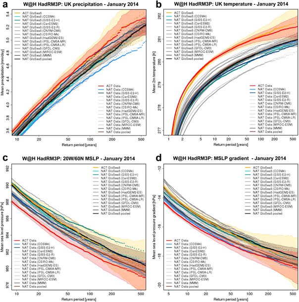
Figure 1. Return time plot for OSTIA and GloSea5 ACT and NAT experiments for January 2014 monthly mean precipitation (a), mean near-surface temperature (b), MSLP at 20° W and 60° N (c), and MSLP gradient between 57° N and 51° N (8° W) (d). Individual actual ensembles are represented by grey dots. CCSM4 (light green and light blue, resp.) and GISS-E2-H (dark green and dark blue, resp.) are highlighted as they show the strongest/weakest response in terms of change in return time for monthly mean precipitation (a). The pooled natural ensembles are highlighted in brown (OSTIA) and black (GloSea5). The 5%–95% uncertainty range is provided for the actual and the pooled natural ensembles.
Download figure:
Standard image High-resolution image
Figure 2. Left column: W@H HadAM3P MSLP anomaly for October 2015 (reference period 1986–2014) for the OSTIA ACT (a), OSTIA NAT (d), GloSea5 ACT (g) and GloSea5 NAT (j) experiment. Middle column: corresponding NCEP Reanalysis 200hPa zonal wind (b) and MSLP anomaly (k) for October 2015. In between the observed OSTIA (e) and GloSea5 forecast SST anomalies (h; forecast issued in August) that we used to force the model experiments (naturalized with CMIP5 SST patterns in NAT cases). Right column: same as left colum but for 200hPa zonal model wind anomalies for October 2015.
Download figure:
Standard image High-resolution imageThe setup necessary to validate the real-time attribution capability consists of four sets of ensemble simulations: two under current climate forcings (ACT) using observed SSTs/SICs (OSTIA [9]) and seasonal forecast SSTs/SICs (GloSea5) and two under natural conditions (NAT) for the two different sets of SSTs. For ACT, the IPCC AR5 RCP4.5 forcing scenario is used and for NAT, the IPCC historical forcing for 1900 is used. While there is only one realization of observed SSTs, the seasonal forecast SSTs are in itself an ensemble obtained by coupled climate models. The atmospheric initial conditions are provided from previous model experiments to ensure consistent spin-up. Variability is introduced using initial condition perturbations. In order to quantify the dynamic model response, a AGCM climatology simulation over the 1986–2014 period (CLIM) with corresponding observed forcing conditions (historical forcing until 2005, IPCC AR5 RCP4.5 forcing afterwards) and prescribed OSTIA SSTs and SIC was run. We use 200 model ensemble member for each year in this case.
GloSea5 is a seasonal forecast product derived from the UK Met Office HadGEM3 GCM [33], coupled with nucleus for European modelling of the ocean (NEMO) ocean [16]. Climate forcings are set to observed values for the hindcast period up to 2005 and follow the IPCC AR5 RCP4.5 scenario afterwards, consistent with our HadAM3P ACT and CLIM setup. It consists of 42 forecast members, corresponding to the forecast runs made in the three weeks (twice daily) before the latest monthly seasonal prediction is issued publicly online. The forecast members are disseminated by the UK Met Office as a monthly data package which also includes ∼12 × 14 yr (1996–2009) of hindcast ensemble simulations for SST for the forthcoming six months.
Being a forecast product from a free running coupled ocean-atmosphere GCM ensemble prediction system, it is susceptible to deviations from the atmospheric mean state after initialization, which, averaged over an ensemble of model runs, lead to systematic SST forecast biases that we have to account for. The UK Met Office has developed its own dedicated bias correction method, using the hindcast ensemble following the procedure described in [1, 15]. End users then have to develop their own bias correction method. We apply a slightly simplified method (no noticeable difference when compared with the UK Met Office method), using the hindcast ensemble average SST for each year and each month to then calculate the difference with observed OSTIA SST for the same month. In the final step, the multi-year average SST difference is applied to the forecast ensemble member of each respective month. For our test case, the England winter floods 2013/14, the GloSea5 forecast issued in November 2013 for December 2013 to May 2014 is used. In figures A1(a) and (c), the OSTIA and GloSea5 SST anomalies for January 2014, relative to the 1996–2009 average, are plotted. ΔSST between OSTIA and GloSea5 (essentially the forecast error) is shown in figure A3(d). The SST anomalies and the forecast error for December and February are very similar in spatial extent and magnitude (not shown). Sea ice extent used in our GloSea5 ACT simulations is directly derived from SSTs. If the grid box average SST is <271.4 K, this box is assumed to be covered with sea ice.
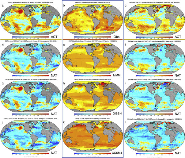
Figure A1. Left column: Analysed OSTIA SST for January 2014 as used for the ACT experiment (a). OSTIA minus the difference between ACT and NAT CMIP5 Multi-Model-Mean SSTs for January 2014 as used in the NAT experiments (d). Same as for MMM in (b) but with GISS-E2-H (g) and CCSM4 SSTs (j). Middle column: HadISST1 observed linear SST trend from 1870-2015 (b). MMM (e), GISS-E2-H (h) and CCSM4 (k) ACT-NAT SST patterns before subtraction from the observed/forecast SSTs. Right column: Forecast GloSea5 SST for January 2014 as used in the corresponding ACT experiment (c). GloSea5 minus difference between ACT and NAT CMIP5 MMM (f), GISS-E2-H (i) and CCSM4 SSTs (l) for January 2014 as used in the GloSea5 NAT simulations. GISS-E2-H and CCSM4 are at the high and the low end of the OSTIA NAT simulations in term of change in return time of (extreme) precipitation events in comparison to the OSTIA ACT experiment.
Download figure:
Standard image High-resolution image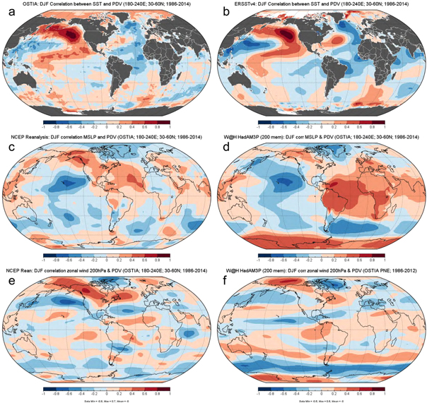
Figure A2. Left column: correlation coefficient between SSTs in NE Pacific region (180°–240° N and 30°–60° N) with OSTIA SSTs (a). Correlation between PNE SSTs and NCEP Reanalysis MSLP (c) and zonal wind speed at 200hPa (e). Right column: same as (a) but for ERSSTv4 SSTs (b). Same as (c) and (d) but for MSLP (e) and zonal wind speed speed (f) from W@H HadAM3P model. Reference period is 1986—2014 and DJF mean is shown in all plots.
Download figure:
Standard image High-resolution imageThe NAT SST patterns are calculated by removing the modelled anthropogenic warming from the observed and seasonal forecast SSTs. To achieve that, we use 11 GCM simulations from the Coupled Model Intercomparison Project phase 5 (CMIP5) archive, averaging and subtracting the monthly climatologies (1996–2005) of the ACT (Historical) and the NAT (HistoricalNat) simulations. The resulting anomaly patterns represent 11 estimates of the possible impact of human GHG emissions on SSTs. They are used to generate the NAT SSTs and to run the associated NAT experiments, along with pre-industrial atmospheric GHG concentrations. In figures A1(d)–(l), the NAT patterns from the multi-model-mean (figure A1(d)–(f)), GISS-E2-H model (figures A1(g)–(h)), and CCSM4 model (figures A1(j)–(k)) are shown. See also figure S3 in [26] where all 11 NAT patterns are provided. HadISST1 [24] linear SST trend (1870–2015) is shown for context as well (figure A1(b)).
3. Results
We focus on the comparison of five RCM ensembles forced with OSTIA and GloSea5 SST/SIC, respectively. For the analysis, ∼17.000 ACT and 11 times ∼10.000 NAT runs with OSTIA SSTs, ∼12.000 ACT and 11 times ∼8.000 NAT runs with GloSea5 SSTs, and ∼6000 ACT CLIM simulations forced with OSTIA SSTs are used. We confine the attribution study to January 2014 as it was the wettest such month in the observed record then (5.2 mm d−1 on average over 8 selected Southern England weather stations extracted from the UK Met Office digital archive), approximately 10% above the previous record, whereas DJF was wettest only by a small margin. For the evaluation of the CLIM experiment, we use all winter months.
We investigate the changes in return times of monthly mean precipitation and near-surface temperature due to anthropogenic forcing in January 2014 (figures 1(a) and (b)), followed by the analysis of the large-scale dynamic setup. We use a MSLP index over the North Atlantic (NA) as well as a meridional MSLP gradient west of the UK in an attempt to disentangle the contribution of changes in thermodynamic and large-scale dynamic processes (figure 1(c) and (d)). The analysis is supported by a model validation exercise with regard to known atmospheric teleconnections in response to anomalous low-frequency SST patterns. Our study region over Southern England is defined from 50° to 52° N and 6.5° W to 2° E in the RCM.
3.1. Thermodynamic/anthropogenic response
Precipitation and near-surface temperature are the most common metrics to estimate the change in atmospheric thermodynamics in response to any given change in external forcing. For January 2014, the observed average rainfall of 5.2 mm d−1 has an estimated return time, based on all available observed NDJF data, of 85 yr (figure 5(c) in [26]). Using ACT and NAT simulations from the OSTIA RCM ensemble, our best estimate for the change in risk of a (natural) 1-in-a-100-year January rainfall event to occur is an increase of 42% (now a 1-in-a-70-year event; figure 1(a)). Individual NAT ensemble members show a wide range between no change (GISS-E2-H) and 160% increase (CCSM4). Using CLIM results (relative to 1986–2011 climatology), [26] found that the modelled January 2014 precipitation and near-surface temperature anomalies are similar to observations for the top 1% wettest (i.e. 1-in-a-100-year return time) in the OSTIA ACT simulations. Despite a notable wet bias (∼0.4 mm d−1) in the RCM in all winter months over southern England, this result is evidence for a reliable representation of the temporal precipitation variability in the model in agreement with previous model evaluation efforts [17].
Consistent with these results, for a 1-in-a-100-year January rainfall event, our GloSea5 results indicate an increasing risk of 66% (now a 1-in-a-60-year event; figure 1(a)). The return times for precipitation are very similar in magnitude, both in the OSTIA and the GloSea5 ACT ensemble. While the pooled GloSea5 NAT ensemble gives a comparable result to OSTIA, individual GloSea5 NAT experiments do different responses owing to different SST patterns. It is exemplified by CCSM4 and GISS-E2-H which show the strongest and weakest signal in case of OSTIA, respectively. We discuss the cause for the difference in the signal associated with the SST patterns shown in figure A1(g) and A1(j) in section 3.4.
For near-surface temperature (figure 1(b)), OSTIA and GloSea5 results provide a comparable and very robust attribution result. Albeit being a fairly moderate month in terms of observed near-surface temperature anomaly, January 2014 was still warmer than average (relative to 1981–2010 in the Central England Timeseries) with a mean temperature of 279.4 K (+1.3 K anomaly). The return time for such an event would have changed from 1-in-a-14-year event under pre-industrial conditions to a 1-in-a-3-year event under current conditions, which corresponds with a more than four-fold increase in probability of such a moderately warm January. The result for the change in risk is essentially the same using GloSea5 forecast SST rather than OSTIA observed SST. Individual NAT simulations show the same magnitude of temperature response to a change in forcing for both, the OSTIA and the GloSea5 experiments.
3.2. Case specific dynamic response
Here, we first analyse the changing return times of MSLP for 20° western longitude and 60° northern latitude (figure 1(c)), the grid point coinciding with the centre of the record low pressure as observed in January 2014 (figure 1(a) in [26]) and hence chosen as an index.
In contrast to the OSTIA ensemble (ACT = red; pooled NAT = brown), in the GloSea5 simulations (ACT = yellow; pooled NAT = black) we find that the risk of such low pressure occurring under ACT conditions does not change for a 1-in-a-100 year event in a NAT world. The OSTIA forced simulations suggest an increasing risk of 33%. We obtain more coherent results when we look at a larger domain over the NA from 38° to 62° N and 8° to 32° W (not shown). In both, the OSTIA and GloSea5 experiment, the risk for a 1-in-a-100-year low pressure situation occurring is not changed significantly between NAT and ACT results.
Analysing the meridional MSLP gradient to the west of England and Scotland (which is considered less sensitive to the selection of the location and at least partly representative of potential changes in the atmospheric circulation over the NA region), we find that a 1-in-a-100-year event in terms of pressure gradient strength in the NAT scenario becomes a 1-in-a-60-year event under ACT conditions using OSTIA SSTs (figure 1(d)). With GloSea5 SSTs, a 1-in-a-100-year event (NAT) becomes a 1-in-a-80-year event (ACT). The risk for a wetter winter under ACT conditions occurring due to a stronger pressure gradient is higher in the OSTIA experiment, which intuitively suggests a stronger dynamic component. Note that the difference between the changing risk in OSTIA and GloSea5 is not significant though.
3.3. Atmospheric teleconnections
It can be shown, as discussed in the
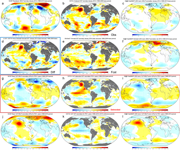
Figure A3. Top row: mean sea level pressure (MSLP) anomaly for January 2014 (reference period 1986–2012) from NCEP Reanalysis (a) and W@H HadAM3P model forced with OSTIA SSTs (c). It is contrasted with the analysed SST anomalies for January 2014 from OSTIA (b). The reference period is 1996–2009, which corresponds with the hindcast period of GloSea5. Middle row: ΔSST between OSTIA and GloSea5 forecast SSTs for January 2014 (d). Note the underestimation of positive SSTs in GloSea5 in the PNE region. GloSea5 forecast SST anomalies for January 2014 (e). On the right, MSLP anomaly from W@H HadAM3P model forced with GloSea5 SSTs (f). Bottom two rows: DJF MSLP anomaly for all PDV positive/negative years (1986–2014 reference period) from NCEP Reanalysis (g/j) and W@H HadAM3P model forced with OSTIA SSTs (i/l). Between the two the corresponding detrended/non-detrended OSTIA SST anomaly for DJF during PDV positive/negative years (h/k). Model experiments are forced with actual GHG concentrations (ACT).
Download figure:
Standard image High-resolution image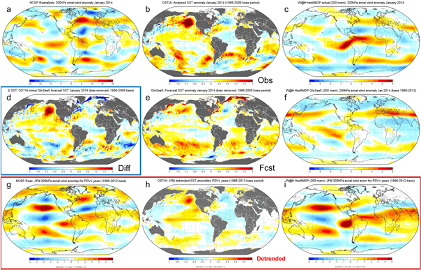
Figure A4. Same as figure A3 but for 200hPa zonal wind speed anomalies. In the bottom row, only the PDV positive case is shown (g)–(i). JFM rather than DJF period is used.
Download figure:
Standard image High-resolution image
While there is evidence that AGCMs tend to produce more or less blocking as a function of Gulf Stream strength [19], and hence the SST gradient in the NA region. Our analysis of the teleconnection strength in HadAM3P suggests that the main cause for the missing NAO/jetstream signal in the GloSea5 ACT experiment is the difference in Pacific SSTs rather than the marginal differences between OSTIA and GloSea5 over the NA. That said, the slightly stronger NA SST gradient in OSTIA may well be caused by the Pacific SST anomaly via a lagged Pacific North American pattern (PNA)-NAO link. The MSLP signal over the NA is, however, almost certainly caused by the direct thermodynamic feedback to SSTs as warmer SSTs cause more buoyant atmospheric conditions, which, on average, lower MSLP.
Noteworthy in this context is that, by construction, the AGCM results (forced SSTs) tend to be damped with regard to higher frequency internal atmospheric chaotic (white) noise due to the fact that thermal air-sea-fluxes are reduced by virtue of disabled air-to-sea heat exchange. In the real world, as well as in fully coupled GCMs such as GloSea5, the high-frequency atmospheric perturbations will interact with SSTs through surface turbulent heat fluxes (air-to-sea) and alter the SST patterns. This is particularly true over the NA region where baroclinicity leads to periods of high cyclonic activity associated with anomalous atmospheric momentum flux and hence surface wind stress [3]. The highly stochastic nature of these processes will inevitably reduce the predictive skill of any set of forecast SSTs. Despite being equally affected by strong baroclinic activity, the Northwest Pacific region is more conducive to persistent SST patterns (as evident in form of ENSO and PDV) as the Walker circulation and the anchoring effect of the Rocky Mountains can lead to constructive or destructive interference between tropical and extra-tropical regions.
If, in contrast to DJF 2013/14, stronger SST anomalies exist, we can actually identify the case-specific dynamic component with our fast-track attribution method. For the ongoing El Niño event of 2015/16, in figure 2 we provide evidence that the dynamic component can be determined with confidence in response to the anomalous Pacific SST pattern for October 2015. We analyse MSLP (figure 2, left column) and 200hPa zonal wind (figure 2, right column) in HadAM3P and NCEP Reanalysis (figures 2(b) and (k)).
The El Niño was well forecast by GloSea5 (August 2015 forecast; figure 2(h); compare with OSTIA in figure 2(e)), which should be expected given the lead time of sub-surface changes in the position of the oceanic thermocline due to anomalous West Wind Bursts months ahead of the actual event. Since extreme events are often linked to anomalous circulation patterns caused by El Niño or La Niña, we are hence able to estimate the increased risk of any given extreme event during such anomalies. The results also suggest that the signal of any potential change of dynamics due to climate change is very small compared to the signal associated with ENSO. In fact, the change in risk for an extreme event occurring owing to case-specific dynamics is very similar in our ACT and NAT experiments (true for both SST scenarios). Notably, even the Reanalysis for October 2015 shows most teleconnection features typical for El Niño, despite being a snapshot of only one month (figures 2(b) and (k)).
3.4. Implications for the risk assessment
Based on our findings so far, here we summarize whether and to what extent we can quantify changes in likelihood for an extreme event occurring as a results of a particularly anomalous dynamic state of the atmosphere:
- Correlation coefficients between tropical or North Pacific SSTs with MSLP and 200hPa zonal wind anomalies (see figure A2) can provide a rough estimate of expected circulation changes as a function of anomalous SST patterns. With OSTIA, the North Pacific SST anomalies in January 2014 are large enough to force a dynamic model response over the NA region. It emerges both at surface level (MSLP) and jetstream level.
- In case of the GloSea5 experiment (ACT), the forecast SSTs do not link strongly with the low-frequency climate modes and the large-scale dynamics over England in January 2014, as the positive SST anomaly in the Pacific is considerably underestimated. In other words, the atmospheric dynamic features triggered by the anomalous NE Pacific SSTs are absent in the model in this case which hampers any attempt to quantify the attributable dynamic component.
- As far as the predictable component with forecast SSTs in more general terms is concerned [20], we find that the associated attribution skill of GloSea5 for PDV-related (Northern Pacific) climate modes is very limited, whereas for ENSO-related (Equatorial Pacific) climate modes it is notably better.
- A promising candidate to quantify the large-scale dynamics impact is the comparison of return times of precipitation from ACT and NAT experiments with the model climatology of the most recent decade (derived from the CLIM experiment). The dynamic component is the difference in return time of precipitation between CLIM and ACT, whereas the thermodynamic component is the difference between CLIM and NAT (expressed in terms of return times in either case). For the UK floods, 20%–30% of the increased risk can be attributed to case-specific atmospheric circulation anomalies in the OSTIA ACT experiment.
- The duration of an extreme weather event is crucial when attributing a dynamic component. Daily events (<3 d) are much less affected by anomalous circulation regimes, hence short extremes are less attributable to atmospheric circulation changes. As for monthly or longer events, the comparison with similar circulation flow regimes can reveal robust attributable results regarding the dynamic component [6]. As demonstrated in [6], investigating DJF and 10 d maximum rainfall over the UK during the winter 2013/14, the change in likelihood of an event occurring in response to anthropogenic/thermodynamic influences can vary by an order of magnitude.
- While the El Niño case of October 2015 suggests a negligible role for event-specific atmospheric circulation anomalies over the UK on the basis of our results (anomalous ACT and NAT MSLP and jetstream patterns are very similar in all experiments; see figure 2), anthropogenic warming is believed to cause (forced) jetstream and circulation pattern shifts to some extent [7, 11].
There is one last point to reiterate. As mentioned in section 3.1, the NAT results differ significantly between different SST patterns. Figures A1(d)–(l) suggest that these patterns vary in the same order as the difference between OSTIA and GloSea5. They may amplify or dampen the signal of a particular climate mode. They may also introduce a stronger or weaker (counterfactual) ocean cooling signal in general. For example, GISS-E2-H (figure A1(g)) amplifies the PDV+ signal in OSTIA in January 2014 (i.e. more precipitation due to enhanced dynamic feedback), while CCSM4 (figure A1(j)) represents the coldest NAT experiment (i.e. much less precipitation due to greatly enhanced thermodynamic signal). The fact that we can identify and disentangle internal dynamic and forced thermodynamic causes when it comes to explaining the difference in the attribution result of individual NAT experiments (due to their characteristic CMIP5-based SST pattern), further increases the confidence in our results, despite the apparent increase in uncertainty expressed in terms of ensemble spread.
4. Conclusions
With the new approach for event attribution introduced in this paper, we show that the coupled GCM-RCM ensemble forced with forecast SSTs and SIC reproduces the attribution result for temperature and precipitation for the England winter flood case, made with the model forced with observed SSTs and SIC. This justifies the suitability of the approach in an operational attribution framework.
When separating the case-specific contribution due to anomalous large-scale dynamic weather patterns, we find that the experiments with forecast SSTs do not give the same answer as those with observed SSTs if the Pacific is not forecast well. The additional analysis of the recent El Niño test case, however, does demonstrate that we can detect potential internal dynamic contributions to a extreme weather case under conditions where SSTs are better predicted. We have also shown that the model reproduces most relevant global teleconnection patterns in response to a major Pacific ocean climate mode, re-emerging in the ensemble mean even on a monthly basis.
Guidance regarding the reliability of the attribution result, particularly over the NA region, is provided by the spread of the individual NAT ensemble experiments. Their impact on the results was demonstrated and could be attributed either to thermodynamic or dynamic causes based on simple physical considerations and the analysis of the teleconnections. Changing SST patterns cause changes in the large-scale dynamics, whereas larger SST anomalies cause a stronger response in form of increased or reduced rainfall.
For the main analysis of the UK winter floods 2013/14, we found that the contribution to the change in risk of the event by changes in the internal case-specific atmospheric dynamics are not reliably detected using forecast SSTs. However, this should not invalidate our rapid attribution result as the thermodynamic changes are the main cause of the increase in risk. This is also true for any forced dynamic contribution due to climate change. Observed SSTs continue to be required in order to gain a comprehensive understanding of the drivers of this particular extreme precipitation event.
We also evaluated the model fidelity with regard to reproduction of atmospheric teleconnection patterns. We found that the dynamic contribution to an extreme event can be detected when particular SST modes exceed a certain thresholds. These findings provide very useful additional guidance regarding the appropriate use of SST data to make predictions about changing risks for certain extreme events, namely those that are related to changes in the atmospheric circulation.
Apart from the standard model validation which concerns the representation of precipitation variability and magnitude [17, 18], the fact that HadRM3P simulates scaling factors for rainfall with temperature over the UK that are in agreement with theoretical considerations (Clausius–Clapeyron scaling in absence of changing atmospheric dynamics), observations [10], and high-resolution model simulations [5] is reassuring with regard to our attribution statement. Nonetheless, biases are still present in the model. With a catalogue of pre-generated global bias data for relevant metrics, we will make sure that we are realistic in what is achievable within the realm of our analysis framework. For example, there may be structural model uncertainty related to underestimated dynamical responses due to missing troposphere–stratosphere interaction as observed in low-top models [25]. We may also discover that forced changes owing to shifts in atmospheric circulation patterns in response to anthropogenic forcing are already contributing significantly to any risk assessment.
Given that there are often conflicting messages and speculations in the immediate aftermath of damaging weather events about whether there is a link to climate change or not, we have demonstrated here that our new method can deliver robust attribution statements as have been frequently requested [29]. It provides a unique opportunity to assess a multitude of extreme weather events in real-time, which, if carefully communicated, has the potential to provide scientific evidence in a debate that otherwise would be dominated by opinion.
Acknowledgments
We thank A Scaife and three anonymous referees for their valuable comments which helped to improve the manuscript. We would like to thank our colleagues at the Oxford eResearch Centre: A Bowery, J Miller and D Wallom for their technical expertise. We would also like to thank all of the volunteers who have donated their computing time to climateprediction.net and W@H. The data for this paper are available by request from the corresponding authors.
Appendix
Given the non-significant nature of changes in MSLP in both, the GloSea5 and OSTIA experiment, here we analyse the model response to anomalous SST patterns associated with major climate modes. In figure A1, the resulting SST anomalies after 'naturalizing' the observed SSTs are shown to put the variability in context of the climate mode variability. This analysis enables us to put the results over the NA region into a global perspective and will also be able to determine the models fidelity to reproduce observed atmospheric variability. NCEP Reanalysis is used as a surrogate for observations. It should be noted that all modes of NH atmospheric variability (e.g. maximum of Jet position, blocking frequency and duration, NAO power spectrum) are well represented [18]. There are regions where the model does have a bias with respect to observation, [17] but these biases tend to have the same magnitude in ACT and NAT model simulations which is why we are confident that existing biases do not compromise our attribution statements.
We focus on the anomalies of MSLP, 500hPa Geopotential and 200hPa zonal wind to the two modes of the PDV/PDO. PDV is thereby defined as the leading Principal Component (PC1) of North Pacific monthly SST variability. We have sub-divided the climatology period into years of the positive (PDV+; 10 yr) and the negative PDV phase (PDV–; 12 yr), respectively. For each year and month, we use an ensemble of 200 HadAM3P global model members. The strategy enables us (1) to identify regions where we can attribute extreme events more reliably and (2) to determine the magnitude of the atmospheric model response in comparison with observations.
In figure A2 (left and middle column), the correlation of OSTIA (figure A2(a)) and ERSSTv4 SSTs (figure A2(b)) with detrended NE Pacific SSTs (180°–240° E and 30°–60° N) is shown for the winter season (DJF). The correlation of global with NE Pacific MSLP and global with NE Pacific 200hPa zonal wind speed is shown in figure A2(c) (NCEP)/figure A2(d) (W@H) and figure A2(e)/(f), respectively. Most of the correlation patterns found in the Reanalysis are also present in the model. Differences are most pronounced in the equatorial Atlantic (model shows stronger coupling with the NE Pacific SSTs) for MSLP and south of 30° S for both, MSLP and 200hPa zonal wind. The correlation is stronger in Reanalysis over North America and the NA region. Dynamically, the link is established by baroclinic waves forming the NA storm tracks in response to geopotential height anomalies associated with negative PNA [23], which projects on the PDV+ pattern. As a result, the MSLP response to PDV between model and Reanalysis is very different over the NA as evident from figure A3(k) (SST pattern), A3(j) (NCEP), and A3(l) (W@H) for PDV–. For PDV+, the problem is less distinct (figures A3(g)–(i)). NCEP clearly shows an increased MSLP gradient (figure A3(g)) which is indicative of a downstream link between PNA (negative) and the (NAO; positive) indeed. The model on the other hand shows a much weaker response and a displacement of the MSLP anomalies to more equatorial latitudes (figure A3(i)).
Since the NA is the very region where we focus with our test case, we explore the large-scale dynamics in more detail. Per definition, the strength of the MSLP gradient determines the NAO phase, which in turn is dynamically controlled by upper level winds, mainly through large-scale modulations of the normal patterns of zonal and meridional heat and moisture transport [12]. More precise, the MSLP anomalies are the surface manifestation of jetstream anomalies that control the cyclonic activity (formation of baroclinic Eddies) over the NA. Therefore, on average the jetstream anomalies should coincide with the MSLP. Since low-frequency atmospheric circulation anomalies are barotropic, mid-troposphere Geopotential (500hPa) and MSPL anomalies are largely proportional [23], we focus on MSLP for the remainder of this analysis. One region where 500hPa Geopotential anomalies do have a much stronger signal during PDV+ is the northeasternmost corner of the Pacific and West Canada, associated with a sometimes 'ridiculously resilient ridge' which can cause harm not only in California [31].
Comparing figures A3(g) and A4(g), the strongest MSLP gradient anomalies are firmly linked to the highest positive jetstream anomalies. Both Reanalysis and model agree very well over the North Pacific, which is particularly remarkable as we are comparing 200 model simulations with one pseudo-observation for PDV+ years. Yet, the magnitude of the anomalies is almost identical. In fact, the model ensemble mean converges very quickly (10 randomly picked ensemble member are already sufficient). This is also the reason why the magnitude of the anomalies in NCEP and HadAM3P is so similar. 10 yr are enough to filter out almost all higher-frequency noise. Over the NA region, the jetstream anomalies show the same general pattern with preponderance of NAO+ conditions during PDV+ winters (PNA–). Lacking a strong NA–MSLP gradient, the 200hPa zonal wind speed in the model is weaker over the NA as well. Interestingly, model and Reanalysis agree better with regard to jetstream anomaly strength over the NA for PDV–years during which baroclinicity is reduced and hence the NAO more negative on average (not shown). It is less surprising given that the MSLP gradient is similar in model and Reanalysis (despite the absolute MSLP values being different; see figures A3(j) and (l)).