
Abstract
A necessary condition for a good probabilistic forecast is that the forecast system is shown to be reliable: forecast probabilities should equal observed probabilities verified over a large number of cases. As climate change trends are now emerging from the natural variability, we can apply this concept to climate predictions and compute the reliability of simulated local and regional temperature and precipitation trends (1950–2011) in a recent multi-model ensemble of climate model simulations prepared for the Intergovernmental Panel on Climate Change (IPCC) fifth assessment report (AR5). With only a single verification time, the verification is over the spatial dimension. The local temperature trends appear to be reliable. However, when the global mean climate response is factored out, the ensemble is overconfident: the observed trend is outside the range of modelled trends in many more regions than would be expected by the model estimate of natural variability and model spread. Precipitation trends are overconfident for all trend definitions. This implies that for near-term local climate forecasts the CMIP5 ensemble cannot simply be used as a reliable probabilistic forecast.
Export citation and abstract BibTeX RIS

Content from this work may be used under the terms of the Creative Commons Attribution 3.0 licence. Any further distribution of this work must maintain attribution to the author(s) and the title of the work, journal citation and DOI.
1. Introduction
Climate projections are often seen as forecasts, especially for the short lead time period in which the differences between emission scenarios are small. The uncertainties up to 2050 are dominated by natural variability of weather and climate, and model uncertainty, the extent to which climate models faithfully represent the real world. On the regional and local scales, where climate information is most often useful, the uncertainties are often taken to be given by the spread of a large climate model ensemble (e.g., van den Hurk et al 2007), which includes both the model estimate of the natural variability and the spread between models. The ensemble is considered to be an estimate of the probability density function (PDF) of a climate forecast. This is the method used in weather and seasonal forecasting (Palmer et al 2008). Just like in these fields it is vital to verify that the resulting forecasts are reliable in the definition that the forecast probability should be equal to the observed probability (Joliffe and Stephenson 2011). If outcomes in the tail of the PDF occur more (less) frequently than forecast the system is overconfident (underconfident): the ensemble spread is not large enough (too large). In contrast to weather and seasonal forecasts, there is no set of hindcasts to ascertain the reliability of past climate trends per region. We therefore perform the verification study spatially, comparing the forecast and observed trends over the Earth. Climate change is now so strong that the effects can be observed locally in many regions of the world, making a verification study on the trends feasible. Spatial reliability does not imply temporal reliability, but unreliability does imply that at least in some areas the forecasts are unreliable in time as well. In the remainder of this letter we use the word 'reliability' to indicate spatial reliability.
This problem was approached in a similar way in two previous studies. Räisänen (2007) showed a global comparison of modelled linear trends (1955–2005) in temperature and precipitation over land in the CMIP3 multi-model ensemble to observed trends. Considering the frequency of cases in which the verification fell outside the forecast distribution, he found that only the temperature trends were compatible with the ensemble spread, precipitation trends were not. Yokohata et al (2012) verified this more formally over the shorter period 1960–1999 using the rank histogram, which indicates how often the observed trend falls in percentile bins of the probability distribution obtained from the model ensemble (Joliffe and Stephenson 2011). Among many measures of the mean state they also included linear temperature trends, which were found to be reliable in CMIP3. Using a different method, Sakaguchi et al (2012) show that the spatial variability of the simulated temperature trends in the CMIP5 ensemble is not large enough. Bhend and Whetton (2012) find that the observed local temperature and precipitation trends are not compatible with the ensemble mean within the observed natural variability, without taking model spread into account. Regional verification studies are discussed in section 4.
Our analysis differs in that we use the more recent CMIP5 ensemble and include the years up to 2011. We also use a different trend definition to improve the signal/noise ratio. In addition, we employ a definition that factors out the global mean climate response to isolate the pattern of climate change that multiplies the global mean temperature change. This addresses the more stringent test whether the regional temperature trends are reliable relative to the global mean temperature trend.
2. Data and methods
The CMIP5 historical runs (Taylor et al 2011) up to 2005 are concatenated with the corresponding RCP4.5 experiments for 2006–2011 to cover the observed period. We use Nmod = 37 models with in total 91 realizations. Multiple realizations of the same model are assigned fractional weights so that each model or physics perturbation has equal weight. Temperature fields have been interpolated bilinearly to a 2.5° grid, for precipitation a conservative remapping was used.
For temperature the GISTEMP analysis with 1200 km decorrelation scale (Hansen et al 2010) is used over 1950–2011, during which the observations are most reliable. This dataset contains SST rather than 2 m temperature over the ocean, but the differences in trends are negligible in the models. The results were checked against the NCDC merged analysis (GHCN v3.2.0/ERSST v3b2, Peterson and Vose 1997) and HadCRUT4.1.1.0 (Morice et al 2012). The equivalent figures for these datasets are available in the supplementary material (available at stacks.iop.org/ERL/8/014055/mmedia).
For precipitation we used the 2.5° GPCC v6 analysis over 1950–2010 (Schneider et al 2011). Boxes with no observations were set to undefined. Results were validated against the CRU TS 3.10.01 analysis (1950–2009) averaged to 2.5° (Mitchell and Jones 2005). Again, we only note features common to both datasets.
Prior to the satellite era analyses south of 45°S are based on very few observations and therefore inaccurate. We therefore exclude this region from the computation of the rank histograms. We show results for the annual mean of all quantities.
For the rank histograms we have to convert the ensemble into a forecast probability. We start by using only a single ensemble member from each model. In that case a definition that works well in conjunction with the rank histogram is to assign a probability 1/(Nmod + 1) to each interval between ensemble members and also to the area below the lowest member and above the highest member. (Note that the probability assigned to the tails is arbitrary, another common choice is to use 1/(2N) for the tails and 1/N for the N − 1 intervals. Alternatively parametric fits or kernels can be used.) The percentile pi of the observed trend in the ensemble is linearly interpolated between the two ensemble members between which it falls, or set to 100/(Nmod + 1)% if it falls below the lowest ensemble member, 100 N/(Nmod + 1)% if it falls above the highest member.
An obvious extension to the case in which there are multiple ensemble members for all models is to give a weight wi = 1/Nens,i to all ensemble members of model i. In case these weights are equal this simplifies to the original formulation. If they are not equal the weight given to each model stays the same ('model democracy'). The remaining problem is which weight to assign to the tails. We have chosen to use a probability w1/(Nmod + wN) for the probability that a trend falls below the lowest ensemble member and N/(Nmod + wN) that it falls above the highest ensemble member. When the trend falls within the ensemble, the probability is again linearly interpolated between the points ni/(Nmod + wN) and (ni + wi+1)/(Nmod + wN) with ni the summed weight of all members with trends lower than observed. This definition puts less weight in the tails, so we verified that all results are also valid in the definition that uses only a single ensemble member from each model.
The pi are collected in a histogram. Ideally this rank histogram should be flat, in which case the forecast probability is equal to the observed probability: each bin j of forecast probability p running from pj to (pj + Δ) then has the same observed frequency Δ.
3. One grid point
The method to compute the rank histograms is illustrated at a single grid point. For this we take The Netherlands, where homogenized temperature and precipitation series are available (van der Schrier et al 2011, Buishand et al 2012). The first trend definition we consider is the linear trend, which is used in most studies (Räisänen 2007, Yokohata et al 2012):

with t the time in years and ζ(x,y,t) the residuals of the fit, which include the part of the forced response that is not linear in time as well as the natural variability on all timescales with mean zero. The trends C(x,y) are determined using a least-square regression, which implies that we assume that the ζ(x,y,t) are normally distributed.
In figures 1(a) and (b) a histogram for linear trends over the period 1950–2011 is shown for the observations and the CMIP5 ensemble. The temperature observations are on the high side of the ensemble: 84% of the models have a trend that is lower than the observed one of 0.024 K yr−1. For precipitation, 98% of the models has a lower trend than the observed 0.21% yr−1 change (van Haren et al 2013).
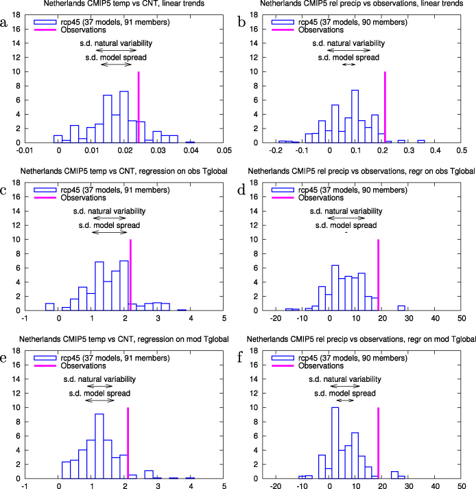
Figure 1. (a) Trend in the homogenized central Netherlands temperature over 1950–2011 compared to the CMIP5 ensemble interpolated to 52°N, 5°E using a linear trend definition (K yr−1). (b) Same for the homogenized Netherlands precipitation (% yr−1). (c, d): As (a, b) but with the trend defined as the regression on the low-pass filtered observed global mean temperature, equation (2) (K K−1), (% K−1). (e, f): As (c, d) but using the modelled global mean temperature, equation (3).
Download figure:
Standard imageThe figures also show an estimate of the (unforced) natural variability σnat around the linear trend, deduced from the intra-model spread of those models with four or more ensemble members. The model spread σmod is estimated from the difference between the full ensemble spread σtot and this estimate,  . As these are based on different model sets the uncertainty in σmod is relatively large. Still, it shows that more than half the ensemble spread is due to the model estimate of natural variability and less than half due to model spread at this location.
An alternative definition of the trend giving a better signal/noise ratio is the change per degree of observed global mean temperature trend (low-pass filtered, in this case with a 4 yr running mean, to filter out ENSO effects):

with A(x,y) the trend and ε(x,y,t) again the variations around the trend. The amplitude of these are smaller than for a linear trend definition, especially for temperature, as the forced trend has been non-linear over the last 62 years and locally often resembles the global mean temperature trend in shape. Using this definition, the histograms for the trends in The Netherlands look very similar (compare figures 1(c) and (d) with figures 1(a) and (b)). Now 88% of the models have a temperature trend below the observed one, for precipitation 98%.
Inspection of the climate model simulations with high temperature trends in The Netherlands shows that the temperature in these models rises very strongly everywhere, rather than just in western Europe (van Oldenborgh et al 2009). The high trend is connected with a high global mean climate response in these models. This response  has been studied extensively (e.g., Frame et al 2005, Knutti and Hegerl 2008). We separate it from the pattern of climate change B(x,y) that multiplies the global mean temperature change by using the slightly different decomposition (van den Hurk et al 2007, Giorgi 2008, van Oldenborgh et al 2009):

with  again low-pass filtered. By definition, the global average of B(x,y) equals one for each model, whereas the average of A(x,y) is related to the climate response of each model. The pattern B(x,y) therefore measures whether the model can simulate regional differences in climate change. Using this definition, 94% of the CMIP5 model experiments have a temperature trend lower than the observed trend in the Netherlands. For relative precipitation trends the fraction is 96%.
Although the observed temperature and precipitation trends at this grid point are high compared to the CMIP5 ensemble (van Oldenborgh et al 2009, van Haren et al 2013), this could well be a coincidence: on a world map, we expect roughly 5% of the grid points to show observed trends that are higher than 95% of the models. To draw conclusions on the reliability of the ensemble we therefore repeat the exercise at all grid points with observations and collect the results in a rank histogram (weighed by grid box size). The expected fluctuations around a flat line due to both model estimates of natural variability and model differences are estimated by taking the first ensemble member of each model in turn as truth. The width of this distribution is computed for each bin of the histogram as in Annan and Hargreaves (2010). This procedure checks whether the observations are as similar to the climate models as the climate models are to each other, and therefore takes into account the spatial autocorrelations of all fields.
4. Global results
We start again with a common trend for all climate models, the regression on the low-pass filtered global mean temperature A(x,y) in equation (2). In figure 2 we show the trends in the observations, GISTEMP (Hansen et al 2010) and GPCC v6 (Schneider et al 2011) (top row), in the CMIP5 multi-model mean (second row), and for each grid point we show the percentile p of the CMIP5 ensemble that is lower than the observed trend (note the non-linear scale). In the grid point corresponding to The Netherlands the GISTEMP trend is slightly lower than the trend of the homogenized Central Netherlands temperature, so that the percentile is just below 80%. (HadCRUT4 uses the homogenized time series for The Netherlands and reproduces the result of figure 1 in this grid point, see supplementary material available at stacks.iop.org/ERL/8/014055/mmedia) The most notable feature in the trends maps is the lack of warming over most of the Pacific Ocean, which is not reproduced by the CMIP5 model mean. In the North Pacific the observed cooling trend is not only lower than the mean, but also falls outside the spread of the ensemble. Much of the Caribbean Sea and western (sub)tropical North Atlantic Ocean has also warmed slower than in more than 95% of the models. However, the areas falling below the 5% rank cover no more than 10% of the globe north of 45°S. This falls well within the bandwidth expected by chance: the 90% confidence limits that are denoted by the grey area in the rank histograms.

Figure 2. Observed trends 1950–2011 in (a) GISTEMP temperature (decorrelation scale 1200 km) (K K−1) and (b) GPCC precipitation (% K−1) as regression on the observed global mean temperature equation (2) (white areas do not have enough data to compute a trend); (c, d) corresponding CMIP5 multi-model mean trends; (e, f) percentile of the observed trends in the CMIP5 ensemble at the same grid point; (g, h) red line: rank histograms of GISTEMP temperature and GPCC precipitation trends versus the CMIP5 trends north of 45°S, grey area: the 90% range obtained from the inter-model variations.
Download figure:
Standard imageThe flatness of the temperature trend rank histogram confirms for the CMIP5 ensemble earlier findings (Räisänen 2007, Yokohata et al 2012) that the temperature rank histograms are flat when taking the same reference for each model, equation (2). However, this does not mean that the ensemble is reliable. The map of figure 2(e) shows coherent spatial patterns that seem to point to physical processes rather than statistical fluctuations resulting from weather noise. This is supported by the observation that the climate models that agree with the relatively high trend in The Netherlands did so because of a high global climate response (section 3).
This becomes clear when considering the trend pattern B(x,y) relative to the modelled global mean temperature rather than the observed one (equation (3), figure 3). Using this measure the ensemble is no longer reliable. There are many more areas with very low and very high percentiles in figure 3 than expected by chance: the rank histogram of the observations is outside the 90% envelope spanned by the CMIP5 models. The reliability of the temperature trends in figure 2 is therefore due to the different climate responses of the global mean temperature in the models and not due to a correct simulation of the pattern of warming. For each point separately the models encompass the observations, but the width is large enough for the wrong reason.

Figure 3. As figure 2, but now temperature and precipitation of each model have been regressed against the global mean temperature of that model, equation (3).
Download figure:
Standard imageThe main areas of discrepancies of temperature trends seem to correspond to well-defined regions. The Pacific Ocean Warm Pool (except the cooling South China Sea) and large areas of the Indian Ocean have been warming faster than the CMIP5 models simulate. This disagreement and the effects on the world's weather have been discussed for the CMIP3 ensemble (Shin and Sardeshmukh 2011, Williams and Funk 2011). The western tropical Atlantic Ocean also has warmed faster than modelled. In Asia, the polar amplification extends further south in the observations than in the models. Western Europe also has warmed faster than modelled (van Oldenborgh et al 2009). The main areas where the observed trend is lower than in the CMIP5 ensemble are in the Pacific Ocean and (sub)tropical western Atlantic Ocean. Due to the high natural variability over land in the models the 'warming hole' in the central and southeastern US is well within the model spread in this analysis. The same holds for the lack of warming over the northern North Atlantic Ocean associated with a decline in the meridional overturning circulation (Drijfhout et al 2012).
For precipitation trends, the reliability diagrams show an overconfident ensemble in both trend measures. This only covers land, as we do not have long precipitation observations over sea. The trend towards more rainfall in the central US is outside of the CMIP5 ensemble, as is the wetting trend in the western half of Australia. The latter has been attributed to ozone effects (Kang et al 2011) and aerosols (Rotstayn et al 2012). The observed rainfall trend in northern Europe (van Haren et al 2013) is also on the high side of the CMIP5 ensemble, in agreement with figure 1. West Africa and northern China are drying in contrast to the modelled wetting trends. The latter could be an effect of aerosol pollution (Menon et al 2002) that is not correctly simulated by the models. These are all large, coherent areas, mostly with high-quality observations, where both precipitation datasets agree on the discrepancy (see supplementary material available at stacks.iop.org/ERL/8/014055/mmedia).
5. Conclusions and outlook
We investigated the reliability of trends in the CMIP5 multi-model ensemble prepared for the IPCC AR5. In agreement with earlier studies using the older CMIP3 ensemble, the temperature trends are found to be locally reliable. However, this is due to the differing global mean climate response rather than a correct representation of the spatial variability of the climate change signal up to now: when normalized by the global mean temperature the ensemble is overconfident. This agrees with results of Sakaguchi et al (2012) that the spatial variability in the pattern of warming is too small. The precipitation trends are also overconfident. There are large areas where trends in both observational dataset are (almost) outside the CMIP5 ensemble, leading us to conclude that this is unlikely due to faulty observations.
It is not obvious how the discrepancy affects future projections. There are three possibilities to explain the overconfidence. The low-frequency natural variability could be underestimated by the models. However, up to timescales that can be compared with observations the modelled temperature variability agrees well with the observations (Knutson et al 2013), with amplitudes dropping off to levels well below the trends already at the timescales sampled by the observations. A second possibility is that the discrepancies are due to errors in local forcings or the sensitivity of the models to those forcings. Aerosol forcings are poorly known over much of the period and direct and indirect effects are uncertain. Land use changes are unlikely the main cause given the location of the trend differences. Thirdly, the patterns can differ due to missing or incorrectly represented local effects of greenhouse warming. For near-term projections all three possibilities must be taken into account, longer-term projections are dominated by greenhouse gases.
For future improvements, the mechanisms behind the differing trends have to be identified in order to improve the climate models. For now, the overconfidence of the ensemble has to be taken into account when interpreting CMIP5 data as an estimate of a probability forecast.
Acknowledgments
We acknowledge the World Climate Research Programme's Working Group on Coupled Modelling, which is responsible for CMIP, and we thank the climate modelling groups for producing and making available their model output. The CMIP5 model data have been obtained via the ETHZ sub-archive and are also available on the KNMI Climate Explorer (http://climexp.knmi.nl). The research was supported by the Dutch research program Knowledge for Climate and received funding from the European Union Programme FP7/2007-13 under grant agreement 3038378 (SPECS). FJDR's work was supported by the MINECO-funded RUCSS (CGL2010-20657) project.