
Abstract
There is an urgent need to reduce the uncertainties in remotely sensed detection of phenological shifts of high latitude ecosystems in response to climate changes in past decades. In this study, vegetation phenology in western Arctic Russia (the Yamal Peninsula) was investigated by analyzing and comparing Normalized Difference Vegetation Index (NDVI) time series derived from the Advanced Very High Resolution Radiometer (AVHRR), the Moderate Resolution Imaging Spectroradiometer (MODIS), and SPOT-Vegetation (VGT) during the decade 2000–2010. The spatial patterns of key phenological parameters were highly heterogeneous along the latitudinal gradients based on multi-satellite data. There was earlier SOS (start of the growing season), later EOS (end of the growing season), longer LOS (length of the growing season), and greater MaxNDVI from north to south in the region. The results based on MODIS and VGT data showed similar trends in phenological changes from 2000 to 2010, while quite a different trend was found based on AVHRR data from 2000 to 2008. A significantly delayed EOS (p < 0.01), thus increasing the LOS, was found from AVHRR data, while no similar trends were detected from MODIS and VGT data. There were no obvious shifts in MaxNDVI during the last decade. MODIS and VGT data were considered to be preferred data for monitoring vegetation phenology in northern high latitudes. Temperature is still a key factor controlling spatial phenological gradients and variability, while anthropogenic factors (reindeer husbandry and resource exploitation) might explain the delayed SOS in southern Yamal. Continuous environmental damage could trigger a positive feedback to the delayed SOS.
Export citation and abstract BibTeX RIS

Content from this work may be used under the terms of the Creative Commons Attribution 3.0 licence. Any further distribution of this work must maintain attribution to the author(s) and the title of the work, journal citation and DOI.
Corrections were made to this article on 13 September 2013. A middle initial was added to the third author's name.
1. Introduction
Temperatures over northern high latitudes have risen by about 2 ° C during the three most recent decades, and an even faster warming trend has taken place at high latitudes in the Arctic (Hansen et al 2006), which has resulted in great changes in terrestrial ecosystems (Levis et al 1999, Macias-Fauria et al 2012). Phenological shifts, as one of the preferred indicators of climate change during the 1980s and 1990s, have been widely documented from field observation (e.g. Ho et al 2006, Menzel and Fabian 1999) and satellite data (e.g. Jia et al 2009, Goetz et al 2005, Karlsen et al 2009). However, changes in phenology were reported to be different in magnitude and even in direction among plant species and areas over the Northern Hemisphere and interpretation of trends is uncertain (Ahas et al 2002, Parmesan and Yohe 2003), especially during the past decade (Walker et al 2012, Zeng et al 2011). There is an urgent need to gain a better understanding of the capacity for satellite sensors to detect phenological shifts of high latitude ecosystems in response to climate and land use changes in past decades.
The Yamal Peninsula located in northwestern Russia is divided into four bioclimatic subzones according to mean July temperature (MJT) and net annual primary production (NAPP) (Walker et al 2012), and is considered as one of the best areas in the Arctic for detecting the effects of climate change along a bioclimatic gradient (Walker et al 2005) (table 1, figure 1). The reasons include consistent substrate types across all subzones coupled with an absence of significant topography. In recent decades, remarkable climate and vegetation changes were reported for the region with remotely sensed approaches (Forbes et al 2010, Walker et al 2011). More attention is paid to the region because it is an important source of oil and gas for Eurasia and also has the largest semi-domestic reindeer populations in the world (Forbes et al 2009, Walker et al 2009). In addition, tundra vegetation is considered sensitive to climate change while simultaneously serving as important rangelands for people and their reindeer herds. Monitoring phenological changes will be very important to indigenous Nenets people who rely on reindeer herding, because the timing for the reindeer to get food is crucial. Therefore, it is essential to detect vegetation phenological changes on the Yamal to better understand the interactions between climate, human beings, and vegetation.
Table 1. Key features of four bioclimate subzones on the Yamal (Walker et al 2005, 2012).
| Subzone | Vegetation | MJTa | NAPb | Site |
|---|---|---|---|---|
| B | Prostrate dwarf-shrub | 4–5 | 0.2–1.9 | Ostrov Belyy |
| C | Hemiprostrate dwarf-shrub | 6–7 | 1.7–2.9 | Kharasavey |
| D | Erect dwarf-shrub | 8–9 | 2.7–3.9 | Vaskiny Dachi |
| E | Low-shrub | 10–12 | 3.3–4.3 | Laborovaya |
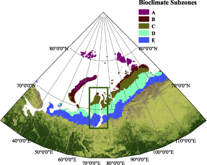
Figure 1. Locations of the Yamal Peninsula study area and the four bioclimatic subzones: subzone B, subzone C, subzone D, and subzone E.
Download figure:
Standard image High-resolution imagePrevious studies on Arctic vegetation phenology have been mostly based on single satellite time series, i.e. AVHRR at 8 km spatial resolution (Jia et al 2004, 2009, Walker et al 2009), leaving major uncertainties due to signal degradation, sensor replacements, and changes of calibration approaches in processing AVHRR time series. Newer time series from later generation sensors onboard polar-orbiting satellites, such as MODIS and SPOT VGT, provide higher accuracy in temporal and spatial resolution for understanding recent phenological changes in northern high latitudes. Thus, we try to make use of data from different sensors and compare their combined derived results. In our study, MODIS and VGT data were used to compare to previous results from single dataset of AVHRR time series.
NDVI as an indicator of the green vegetation is related to vegetation growth status, serves as a strong proxy for gross photosynthesis (Goetz et al 2005), and is a useful tool for the assessment of vegetation (van Leeuwen et al 2006). NDVI values from −1 to 1 show the differences in the reflection between the red and near-infrared portions of the spectrum characteristic of many kinds of land cover categories, such as dense vegetation, sparsely vegetated and bare surface. NDVI has become one of the most common indices used to study vegetation phenology via remote sensing (Jia et al 2004). Thus, NDVI time series derived from AVHRR, MODIS and VGT data were used to investigate changes of vegetation phenology over our study area.
Temperature is considered as the most important factor for plant community distribution and biomass in the Arctic tundra (Epstein et al 2008, Walker et al 2005). Some studies have showed a clear phenological response to global warming year by year (Jia et al 2009, Parmesan and Yohe 2003). An increase in temperature in early spring of 1 ° C can result in an earlier start of the growing season (SOS) by 7.5 days and warming in the autumn of 1 ° C can delay the end of the growing season (EOS) by 3.8 days in temperate vegetation (Piao et al 2006). Reindeer husbandry and resource exploitation were reported to have affected NDVI patterns on most surfaces of the Yamal Peninsula (Walker et al 2009) and might influence vegetation phenology as well. Therefore, both anthropogenic and natural factors are necessary to consider in investigating phenological changes in northern biomes like the Arctic tundra.
We have selected the Yamal as a case study to examine and compare phenological shifts as detected from multi-satellite data and to seek the possible reasons underlying any observed changes. Key scientific questions include: (1) are there any further improvements in detecting phenological parameters including SOS, EOS, length of the growing season (LOS) and MaxNDVI by using multiple satellite time series; (2) what are the probable reasons behind the phenological changes detected in the study area? The key objective of the study is to reduce the uncertainties in remotely sensed detection of phenological shifts of high latitude ecosystems in response to climate changes in the past decade.
2. Data and methods
2.1. Satellite data
AVHRR data from the National Oceanographic Atmospheric Administration (NOAA) polar-orbiting satellites was post-processed by NASA Global Inventory Monitoring and Modeling Systems (GIMMS) group with a spatial resolution of 8 km × 8 km and 15-day temporal resolution from 1982 to 2008 (Bhatt et al 2010, Tucker et al 2005). AVHRR NDVI was calculated from spectral reflectance in visible (R: 0.58–0.68 mm) and near-infrared (NIR: 0.725–1.1 mm) bands as: NDVI = (NIR − R)/(NIR + R). MODIS reflectance product MOD09A1 with a spatial resolution of 0.5 km × 0.5 km and 8-day temporal resolution was processed and provided by the MODIS vegetation team. NDVI transformed from MODIS reflectance data was calculated by visible (R: 0.58–0.68 μm) and near-infrared (NIR: 0.73–1.10 μm) wavelengths as: NDVI = (NIR − R)/(NIR + R). VGT product with a spatial resolution of 1 km × 1 km and a 10-day temporal resolution was available as DN values, and we further calculated NDVI with the equation: NDVI = DN∗0.004 − 0.1. Much narrower bandwidth of red (0.61–0.68) and NIR (0.78–0.89) is used to calculate NDVI from VGT data. VGT data contained parts of subzone C, subzone D and subzone E. The time period of both MODIS data and VGT is from 2000 to 2010.
MODIS land surface temperature products (MOD11C2) at a 0.05° spatial resolution and 8-day temporal resolution were used here to analyze decadal trends of surface temperature. Temperature in the months before SOS and EOS were assumed to be responsible for dynamics of key phenological parameters in northern ecosystems (Jeong et al 2011, Zeng et al 2011). Therefore, we examined correlation coefficients between SOS and monthly averaged temperatures in April, May and June, and correlation coefficients between EOS and monthly averaged temperatures in August, September and October. Correlations of |r| > 0.6 were highlighted in our spatial datasets.
2.2. Analysis of phenological parameters from NDVI time series
Cloudiness products are commonly generated from satellite data. Due to the cloud filtering function of the maximum value composition (MVC) only selects the highest NDVI values (Stisen et al 2007), we chose the TIMESAT software with the smoothing function-Savitzky–Golay filter to further eliminate errors caused by residual cloud and haze effects (Jonsson and Eklundh 2004) (figure 2). Also, to reduce the possible effects of the varying temporal resolution between the three sensors on the seasonal metric calculations, TIMESAT was applied to fit daily NDVI data. The Savitzky–Golay filter replaced the noise values with the average of the values in the window and is powerful for enhancing the quality of the NDVI curve (Jonsson and Eklundh 2004). Thresholds, derivatives, smoothing functions, and fitting model are the main methods for determining phenological parameters from seasonal variations in NDVI (de Beurs and Henebry 2010). In our study, thresholds were chosen as the simplest and most effective for phenological study (de Beurs and Henebry 2010). The thresholds of NDVI values are different among biomes (Reed et al 1994), but the periods with the greatest NDVI increase and decrease were often defined as the start and end of the growing season (Jeong et al 2011, Piao et al 2006). Changes in phenological parameters using the thresholds from NDVI climatology matched changes in climate well over many biomes. NDVIratio was calculated from the NDVI time series derived from different satellite sensors with the equation:

where t is time, which differs among AVHRR, MODIS and VGT data due to different temporal resolutions. The absolute value of the divisor was used in the formula to avoid NDVI(t) changing the sign of NDVIratio(t). For example, when NDVI (t + 1) is greater than NDVI (t), the NDVIratio(t) is positive and will never be negative number because NDVI < 0. The maximum and minimum values of NDVIratio(t) were used as thresholds to determine the average onset of SOS and EOS.
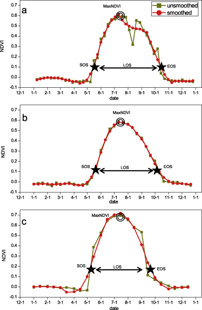
Figure 2. Determination of phenological parameters based on (a) MODIS data, (b) VGT data and (c) AVHRR data from 2001 over bioclimatic subzone E.
Download figure:
Standard image High-resolution imageHere we use TIMESAT to explore and extract seasonality parameters from remotely sensed time series data (figure 2). The parameters are applied in TIMESAT as follows: spike method= 1 median filter, seasonal parameter= 0.5, number of envelope iterations= 1, adaptation strength= 2, Savitzky–Golay window size= 2, absolute value for start season= maximum values of NDVIratio, absolute value for end season= minimum values of NDVIratio. Phenology parameters including SOS, EOS, LOS and MaxNDVI were analyzed with each satellite time series. We focused on vegetated areas, and therefore masked off pixels of water bodies and barren ground where the largest NDVI value throughout the growing season was very low (<0.1).
A t-test and 95% confidence interval was used to identify statistically significant linear trends of the phenology metrics during the study period. SAS software was used to fit auto-regression to examine the temporal patterns of interannual trends and variations. Statistical significance and a 99% confidence interval were used to test the differences between results from pairs of AHVRR, MODIS and VGT satellite sensor data.
3. Results
3.1. Spatial patterns of key phenological parameters
The spatial distributions of the phenological parameters SOS, EOS, LOS and MaxNDVI on the Yamal were calculated from 2000 to 2010 based on the MODIS data and VGT data, and from 2000 to 2008 based on the AVHRR data (figure 3). There were earlier SOS, later EOS, longer LOS and greater MaxNDVI from north to south on the Yamal based on MODIS data and VGT data (figure 3). From AVHRR data, there was not a clear geographical trend of SOS and LOS, though later EOS and greater MaxNDVI were seen from north to south on the region. Phenological parameters in the subzones D and E had similar trends as seen from the MODIS and the VGT data, which were a little different from the parameters based on AVHRR data (figure 3). The SOS dates were distributed from approximately 1 May to 1 July based on MODIS data and VGT data (figures 3(a) and (e)), but were much earlier (mainly before 20 May) based on AVHRR data (figure 3(i)). The EOS date approximately ranged from 1 October to 10 November. The most delayed EOS found on the Yamal was based on AVHRR data (figure 3(j)). EOS in subzone E was similar from MODIS (figure 3(b)) and VGT data (figure 3(f)), while there were almost 10-day differences in other parts of the area. The LOS date ranged from 80 to 150 days. LOS from MODIS (figure 3(c)) and VGT (figure 3(g)) data are very similar in subzones D and E. Compared to LOS based on the other satellite sensors, LOS from AVHRR was greater due to earlier SOS and much delayed EOS, and there were not apparent differences among the four climate subzones (figure 3(k)). MaxNDVI ranged from 0.5 to 0.9. The values of MaxNDVI based on these three sensors were mostly similar, but MaxNDVI from AVHRR was greater in some parts of the subzones D and E (figure 3(l)). From low to high latitudes, clearly delayed SOS and advanced EOS were demonstrated from these three multi-satellite data sources (figure 3), i.e. the spatial distributions of the SOS date were opposite to the spatial distributions of the EOS date.

Figure 3. Spatial distributions of climatology of vegetation SOS, EOS, LOS and MaxNDVI in the Yamal. Results are based on average of MODIS and VGT data during the period 2000–2010, and based on average of AVHRR data during the period 2000–2008. The boundaries of each subzone are shown on each of the subsequent figures.
Download figure:
Standard image High-resolution imageSignificance tests of SOS and EOS among the multi-satellite data were performed (figure 4). AVHRR data were from 2000 to 2008, so the significance tests between AVHRR data and another data set were done over these years to ensure consistency (figure 4). The significance tests were done in regions that VGT has coverage. For SOS, AVHRR time series were significantly different from VGT data in about 86% of the areas within the study region (figure 4(a)) and from MODIS data in 52% of areas within the region (figure 4(b)). The differences in SOS between MODIS and VGT data in most of subzone C, subzone D and subzone E were not significant (almost 90% of the areas) (figure 4(c)). Almost half of the study area showed significant differences in EOS between AVHRR data and VGT data (figure 4(d)). MODIS data did not show significant differences of EOS with AVHRR data (figure 4(e)), and VGT data (figure 4(f)) over a large area.

Figure 4. Correlation significances of SOS and EOS between pairs of MODIS, AVHRR and VGT satellite time series.
Download figure:
Standard image High-resolution image3.2. Phenological changes over the region
Spatial distributions of linear trends of key phenological parameters were examined from 2000 to 2010 based on MODIS data and VGT data, and from 2000 to 2008 based on AVHRR data (figure 5). Positive values indicate later SOS, later EOS, longer growing season, and larger MaxNDVI. As demonstrated from these multi-sensor data, a part of subzone C, and all the areas in subzones D and E experienced positive trends in SOS based on MODIS (87% delayed areas) (figure 5(a)) and VGT (95% delayed areas) (figure 5(e)). SOS in 76% of the areas within the region experienced negative trends as seen from AVHRR data (figure 5(i)). From the south to the north, the shifts of SOS turned from apparent positive trends to slightly positive trends, and to negative trends based on MODIS (figure 5(a)) and VGT (figure 5(e)), while there were no identical latitudinal gradients shifts of SOS from AVHRR data (figure 5(i)). Delayed EOS was found in much of region (72% of areas) except subzone E during 2000–2010 based on the MODIS data (figure 5(b)). Compared to the results from MODIS data, stronger delayed EOS was found based on the AVHRR data in most Yamal areas (figure 5(h)). In contrast, subzone D and subzone E and parts of subzone C experienced an advanced EOS from 2000 to 2010 as seen from VGT data (figure 5(f)). From 2000 to 2010, the combination of delayed SOS and advanced EOS shortened LOS mainly in subzone D and E as seen from VGT (figure 5(g)) and MODIS data (figure 5(c)), while prolonged LOS was also found in some northern regions. AVHRR data (figure 5(k)) showed a lengthened LOS from 2000 to 2008, especially in subzone C and subzone E, which were mainly attributed to the delayed EOS. All three satellite time series showed decreases of MaxNDVI in subzone C and increases of MaxNDVI in subzone D and subzone E. While in subzone B, MODIS data showed increases of MaxNDVI from 2000 to 2010 (figure 5(d)), but AVHRR showed an opposite trend of MaxNDVI from 2000 to 2008 (figure 5(l)).
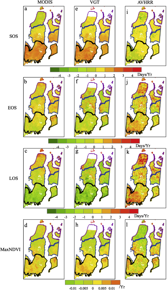
Figure 5. Spatial patterns of the SOS, EOS, LOS and MaxNDVI linear trends from 2000 to 2010 based on MODIS data and VGT data, and from 2000 to 2008 based on AVHRR data. Positive values (warm colors) indicate later onset, later EOS, longer growing season and larger MaxNDVI.
Download figure:
Standard image High-resolution imageVariations of these four phenological parameters on the Yamal and each subzone were averaged to examine the interannual variations (figure 6). The values and trends of phenological parameters based on MODIS and VGT data were similar in subzones D and E. SOS was found to be slightly different in subzone B between MODIS and AVHRR, while the gap between two data sets was almost 20 days in other parts of the region (figure 6(a)). EOS based on MODIS and VGT was nearly the same as the date from AVHRR since 2004, except over the region of subzone B (figure 6(b)). There were different trends of LOS shifts as detected by MODIS data from 2000 to 2010 and AVHRR from 2000 to 2008, except in subzone B (figure 6(c)). SOS was delayed by 12.1 days per decade based on MODIS data (R2 = 0.33), leading to a shortened LOS (table 2). The remarkably delayed EOS by 31.0 days per decade (R2 = 0.52) resulted in an overall lengthening of LOS by 26.6 days per decade (R2 = 0.45) according to AVHRR data. MaxNDVI showed no clear change in the region, except for a slight decrease in subzones B and C. Quite a large difference in MaxNDVI between MODIS and AVHRR could be found in subzone B, while differences were similar in the other parts of the region (figure 6(d)).

Figure 6. Interannual variations of area-averaged (a) SOS, (b) EOS, (c) LOS and (d) MaxNDVI (peak greenness) in the Yamal and its four subzones based on MODIS data (black lines, 2000–2010), VGT data (blue lines, 2000–2010) and AVHRR data (red lines, 2000–2008).
Download figure:
Standard image High-resolution imageTable 2. Shifts of phenology parameters (b: regression coefficient and R2: coefficient of determination) based on MODIS, AVHRR and VGT on the Yamal and each subzone. Significant correlations (p < 0.05) are highlighted in bold.
| Areas | Phenology | MODIS | AVHRR | VGT | |
|---|---|---|---|---|---|
| Yamal | SOS | b/day/decade | 12.1 | 4.4 | |
| R2 | 0.33 | 0.20 | |||
| EOS | b/day/decade | 0.1 | 31 | ||
| R2 | 1.00 × 10⁻⁵ | 0.52 | |||
| LOS | b/day/decade | −12.1 | 26.6 | ||
| R2 | 0.19 | 0.45 | |||
| MaxNDVI | b/decade | −0.013 | 0.006 | ||
| R2 | 0.03 | 0.01 | |||
| B | SOS | b/day/decade | −5.3 | 0.1 | |
| R2 | 0.09 | 5.00 × 10⁻⁵ | |||
| EOS | b/day/decade | 16.1 | 6 | ||
| R2 | 0.44 | 0.27 | |||
| LOS | b/day/decade | 21.4 | 5.85 | ||
| R2 | 0.39 | 0.1096 | |||
| MaxNDVI | b/decade | −2.00 × 10⁻⁵ | −0.116 | ||
| R2 | 4.00 × 10⁻⁸ | 0.5698 | |||
| C | SOS | b/day/decade | −0.7 | 2.0 | |
| R2 | 0 | 0.03 | |||
| EOS | b/day/decade | 1.9 | 25.4 | ||
| R2 | 0.01 | 0.52 | |||
| LOS | b/day/decade | 2.6 | 23.4 | ||
| R2 | 0.01 | 0.37 | |||
| MaxNDVI | b/decade | −0.045 | −0.4 | ||
| R2 | 0.40 | 0.55 | |||
| D | SOS | b/day/decade | 13.8 | 6.5 | 11.6 |
| R2 | 0.35 | 0.17 | 0.40 | ||
| EOS | b/day/decade | 1.1 | 28.1 | 3.0 | |
| R2 | 0.01 | 0.46 | 0.02 | ||
| LOS | b/day/decade | −9.6 | 21.7 | −8.6 | |
| R2 | 0.12 | 0.26 | 0.11 | ||
| MaxNDVI | b/decade | −0.013 | 0.03 | 0.003 | |
| R2 | 0.02 | 0.11 | 0 | ||
| E | SOS | b/day/decade | 18.88 | 4.7 | 16.7 |
| R2 | 0.4655 | 0.13 | 0.51 | ||
| EOS | b/day/decade | −0.204 | 39.6 | 3.9 | |
| R2 | 0 | 0.62 | 0.07 | ||
| LOS | b/day/decade | −19.1 | 34.875 | −12.8 | |
| R2 | 0.40 | 0.6054 | 0.28 | ||
| MaxNDVI | b/decade | 0.016 | 0.003 | 0.035 | |
| R2 | 0.04 | 0 | 0.08 | ||
3.3. Possible drivers for phenological changes
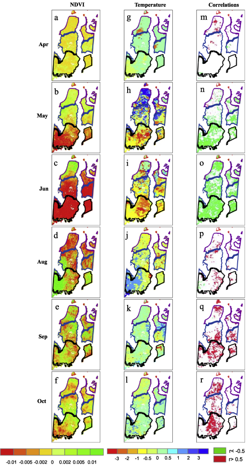
To find out the main drivers behind the phenological changes, we analyzed monthly mean temperatures and NDVI change, and correlation coefficients between phenology and temperatures in these months (figure 7). NDVI decreased over the most areas in April (figure 7(a)), strongly in subzone E in May (figure 7(b)), and in subzone D and E in June (figure 7(c)) from 2000 to 2010 based on MODIS data. During the three months in autumn phenological events, NDVI variations differed in direction across the region (figures 7(d)–(f)). In other words, there were no clear and consistent changes of NDVI in August, September and October from 2000 to 2010. Subzone B and subzone C experienced increasing temperature for April, May and June. A decrease in temperatures was shown in subzone D and subzone E in May (figure 7(h)) and June (figure 7(i)). The temperatures in May (figure 7(n)) and June (figure 7(o)) were negatively correlated with SOS variations over 67% and 85% of the study area, respectively based on MODIS data, which indicated that delayed SOS from MODIS data was related to low temperature in these months. Warming trends were found in September (figure 7(k)) and October (figure 7(l)). Temperature in September and October had strong positive correlation with EOS from MODIS data over near half of the region.
Figure 7. Spatial distributions of climatology of NDVI, temperature and statistical correlations between temperature and SOS in April, May and June and between temperature and EOS in August, September and October. NDVI, SOS and EOS were calculated by 11-year MODIS data. Temperature data were based on MODIS thermal infrared land surface temperature. Here, r > 0.5 (red areas) and r <− 0.5 (green areas) were used to show relatively strong positive and negative correlation.
Download figure:
Standard image High-resolution image
4. Discussion
Different sensors dataset comparison were applied to test the consistency of three satellite datasets over the same region and similar time period, in order to increase confidence in satellite-based detection of phenology changes in the circumpolar Arctic. As described above, absolute values and trends in phenological parameters between MODIS and VGT derived temporal and spatial patterns were generally in agreement. Phenological parameters viewed from AVHRR time series were in many cases different from the results based on the other satellite datasets. The possible reasons as follows: (1) the MODIS/VGT has much narrower red (620–670 nm)/(610–680 nm) and NIR (841–876 nm)/(780–890 nm) bands than the AVHRR red (585–680 nm) and NIR (730–980 nm) bands, which can lead to more sensitive values of NDVI. (2) Inconsistency in data sources would affect the data quality for four different AVHRR sensors (NOAA-14, NOAA-16, NOAA-17 and NOAA-18) used over the last decade, each with a different equator passing time (morning and afternoon satellites are combined) and varying degrees of orbital drift (Tucker et al 2005). (3) Compared to AVHRR, MODIS and VGT have improved onboard geometric and radiometric calibrations (Brown et al 2006). (4) AVHRR data have much lower spatial and temporal resolution than MODIS and VGT data, and resolution can greatly influence the accuracy of phenological detection especially in the Arctic, where seasonal changes occur abruptly (Menzel et al 2006). It has been demonstrated that newer generation sensors VGT and MODIS perform better than AVHRR in phenological analyses in certain ecosystems, such as alpine grasslands (Fontana et al 2008). In addition, because of calibration issues, AVHRR data have rather poor image quality north of 70° N during 2004–2005 (Bhatt et al 2010), which might partially explain the remarkably delayed EOS resulting in huge increases of LOS on the Yamal (figure 5). MODIS and VGT data were considered an improvement over AVHRR, and these products in theory provided a possibility to evaluate NDVI time series for overlapping periods. Therefore, AVHRR data are an important data source for temporal segments from 1981–present, whereas MODIS and VGT data could help improve phenological studies for the most recent decade.
Many previous studies provided similar estimates of advanced SOS and lengthening LOS over Arctic tundra and other biomes in the world (e.g. Jeong et al 2011, Julien and Sobrino 2009). 78% of plant species observed experienced advancing SOS as synthesized from more than 125 000 records of phenological observations during the period of 1971–2000 (Menzel et al 2006). Our study demonstrated delayed SOS in the southern portion of the Yamal. Similar delayed SOS was also reported in other cases in recent years (Delbart et al 2006, Yu et al 2010). Delayed EOS rather than advanced SOS was thought to be the main reason for lengthening LOS by analyzing the time series of AVHRR data in the last decade (Zeng et al 2011, Zhu et al 2012). However, there was no obvious delayed EOS based on MODIS and VGT found in our study. We confirmed gradual increases in MaxNDVI from northern bioclimatic subzones to the south as expected, along the gradient of warmer temperature (Walker et al 2011). It was earlier reported that MaxNDVI has increased slightly during 1982–2007 based on AVHRR data (Walker et al 2011), and from 2000 to 2008 we find the similar trends based on AVHRR data (table 2). In the last decade, MaxNDVI had decreased slightly, especially in subzone B and subzone C based on the MODIS data in our study. MaxNDVI in subzone E has increased from MODIS data and VGT data during 2000–2010. In our study, subzone B is represented only by Belyy Ostrov, an island north of the Yamal Peninsula. The area contains few pixels in this subzone especially from the coarser resolution AVHRR data. This may affect the accuracy of phenological results on the region. Therefore, the phenology trends detected in subzone B of the Yamal may not be applicable to circumpolar subzone B.
Temperature has been considered as one of the most important natural drivers behind vegetation dynamics in Arctic tundra ecosystems (Chapin et al 2000). Warmer temperatures in early spring were considered as the main factor for advanced SOS as previously reported (Ahas et al 2002, Menzel and Fabian 1999). Strong negative correlation coefficients between temperature and SOS in May and June over almost the entire region indicated that cool temperatures during these phases might push SOS backward (figure 7). Therefore, the delayed SOS in the last decade may have been driven by decreased temperatures in May and June.
Warming in Arctic tundra regions has been widely reported (Kaufman et al 2009, Serreze et al 2000). This raises the question, what were the reasons for cooling in the Yamal areas during these months? Firstly, Arctic vegetation provided a negative feedback to warmer temperature by increased carbon dioxide (CO2) uptake due to increased productivity resulting from rising temperature (Serreze et al 2000). However, such a negative feedback from vegetation cover does not appear to have been the driver on the Yamal, as we explain below. Yamal vegetation in subzones C–E has experienced greater pressure relative to subzones A–B from anthropogenic effects such as hydrocarbon extraction and, perhaps, zoogenic disturbances resulting from steady decadal increases in Nenets reindeer herds (Forbes et al 2009). Thousands of square kilometers of pasture in southern and central Yamal-Nenets Autonomous Okrug have been undergoing a fundamental transformation in recent decades due to industrial activities such as the exploration of vast oil and gas deposits (Kumpula et al 2011, 2012). Industrial impacts or climate effects, or a combination of these, has been considered as the main driver affecting Arctic areas underlain with hydrocarbon and mineral deposits (Kumpula et al 2010). Such anthropogenic disturbances resulting in large areas of reduced or altered vegetation cover can be detected by high resolution satellite imagery and have occurred extensively in subzones D and E. NDVI on the Yamal may therefore have been influenced strongly by these disturbances (reindeer pasturing and other social–ecological factors) rather or to a greater extent than land temperatures (Forbes et al 2009). Secondly, strong positive correlations were found between NDVI and temperature in June from 2000 to 2010. NDVI decreased in subzones D and E in May and June from 2000 to 2010 based on MODIS data (figure 7), which may have resulted in an increase of albedo leading to a climate cooling effect. Such a cooling may play an important role in delaying SOS, especially in spring when solar radiation increases in concordance with longer daytime hours. Such a cooling also might lead to lower NDVI values in Arctic tundra, which can be interpreted as a positive feedback to delayed SOS. What is more, the delaying effect may be a manifestation of decreases in NDVI in May and June leading to a later fulfilment of thresholds for SOS. Thus, lower NDVI might be one of the reasons for lower air temperatures during the last decade, and leading to delayed SOS. Previous studies have shown that Arctic warming is an important factor for tundra shrub expansion (Tape et al 2006) and increases in biomass (Forbes et al 2010, Macias-Fauria et al 2012), whereas reindeer herbivory may counteract this response (Olofsson et al 2009). Therefore, anthropogenic factors might be an important reason for delayed SOS in the last decade on the south of the Yamal.
Changing land use and other human activities have become the most fundamental drivers of environmental changes in many parts of the world (Turner et al 2007). Changes in grazing (Yu et al 2003) and farming systems (de Beurs and Henebry 2004) have been reported as key drivers underlying land surface phenological changes in eastern central Asia. In western Arctic Russia, continuous increases in human population and reindeer grazing have probably had a significant effect on tundra vegetation at the regional scale (Walker et al 2011, 2012, Yu et al 2011). Meanwhile, rapid expansion of oil and gas fields and related infrastructures (such as railway, road, camps, warehouse and pipelines) created dense patches of bare scars and tracks in tundra (Kumpula et al 2010, 2011). In many cases, those disturbances were clearly visible even from fine to moderate resolution satellite images (Kumpula et al 2010). Such cumulative anthropogenic impacts have significantly modified vegetation cover in the region in past decade or so (Walker et al 2011). Such intense human disturbances will continue to increase as gas production ramps up in the near future (Kumpula et al 2012) and have the potential to buffer or even alter the climate driven patterns and trends of key phenological parameters at the regional scale.
Warming during the period of EOS (August–October) has resulted in major delays in EOS (Jeong et al 2011). A recent study on the Tibetan Plateau reported that warm temperatures in July and August led to an advanced EOS, and warming in September was related to a delayed EOS (Yu et al 2010). However, on the Yamal there were no clear and consistent changes of temperatures and NDVI in September and October from 2000 to 2010, resulting in no obvious changes in EOS or LOS based on MODIS data. The implications of our findings are important to carbon budgets at a regional scale in spring and autumn. This is because longer LOS is related to greater primary productivity (GPP) and net primary productivity (NPP) in a cycle of the season, leading to variations in atmospheric carbon at a global scale (Piao et al 2007).
5. Conclusions
Multi-sensor dataset integration and comparisons were applied to improve confidence in satellite-based investigations of decadal changes of vegetation phenology in the Arctic. Phenological parameters based on the different satellite sensor data were not consistent in many cases. Although MODIS and VGT data were considered major improvement over AVHRR, and these products provided higher spatial and temporal resolution, there are still biases in those datasets. As for many coarse resolution satellite time series, MODIS and VGT data also suffer from potential cloud contamination (even with MVC weekly composite) and potential calibration errors in red and near-infrared bands due to high solar zenith angles in the Arctic. Also, VGT data become inconsistent and in some cases discontinuous near its northern edge in subzone C. Therefore, land surface observations should be added to examine the accuracy of phenological trends derived from multi-satellite time series. We have offered a range of values and trends of phenological parameters in western Arctic Russia along a bioclimatic gradient (four subzones), and discussed the possible drivers underlying changes documented during the past decade. We suggest that temperature is still the key factor explaining the observed phenological trends and variability. Meanwhile, anthropogenic and zoogenic factors, such as petroleum development and reindeer herbivory, may also have important effects on the decadal shifts in phenology by modifying vegetation cover and snow-albedo feedbacks. Consequently, interactions of ecological, social and atmospheric factors have controlled the vegetation phenology during the last decade over the study region. Field based vegetation spectral measurements will be applied to test the differences in the results based on multi-satellite data in subsequent investigations.
Acknowledgments
This study was supported by the National Natural Science Foundation of China (Grant No. 41176168) and the National Basic Research Program of China (Grant No. 2009CB723904). We thank NASA GIMMS team for providing the most updated AVHRR GIMMS3g dataset. We also thank NASA/MODIS Land Discipline Group and VGTImage/Vito for sharing the MODIS LAND and VGT data.