
Abstract
This study examines the subset climate model ensemble size required to reproduce certain statistical characteristics from a full ensemble. The ensemble characteristics examined are the root mean square error, the ensemble mean and standard deviation. Subset ensembles are created using measures that consider the simulation performance alone or include a measure of simulation independence relative to other ensemble members. It is found that the independence measure is able to identify smaller subset ensembles that retain the desired full ensemble characteristics than either of the performance based measures. It is suggested that model independence be considered when choosing ensemble subsets or creating new ensembles.
Export citation and abstract BibTeX RIS

Content from this work may be used under the terms of the Creative Commons Attribution 3.0 licence. Any further distribution of this work must maintain attribution to the author(s) and the title of the work, journal citation and DOI.
1. Introduction
Ensembles of simulations are used in both weather forecasting and climate modeling. The ensemble mean is often used to synthesize the information present, and has been found to perform better than any individual ensemble member where the mean, rather than variance quantities, is of interest (Gleckler et al 2008, Pierce et al 2009, Pincus et al 2008, Reichler and Kim 2008). Various attempts to improve the ensemble mean through performance based weighting have resulted in only minor improvements (Christensen et al 2010, Räisänen and Ylhäisi 2012). We also note that the success of the multi-model mean as a 'best estimator' is consistent both with a 'truth-centered' interpretation of an ensemble (where observations are assumed at the center of ensemble spread; (Knutti et al 2010, Annan and Hargreaves 2010)) and with the interpretation of the ensemble as a collection of samples drawn from a distribution within which the model simulations and observations are indistinguishable (Annan and Hargreaves 2010, Bishop and Abramowitz 2013, Sanderson and Knutti 2012). However, there is broad recognition that models often share sections of code or whole parametrizations such that they do not provide independent samples (Knutti et al 2010, Pennell and Reichler 2011).
When designing regional climate model ensembles there is always a practical limitation on the number of simulations that can be performed. Thus, one must choose a subset of the possible simulations to perform based on some criteria. For regional climate model ensembles this includes choosing the global climate models (GCMs) from which to downscale, and choosing the regional climate models (RCMs) to downscale with. To date this criteria has been limited to performance measures (e.g. Pierce et al 2009, Nguyen et al 2012), or consideration of the projected future change (McSweeney et al 2012). These different approaches are generally aimed at optimizing the ensemble mean or the ensemble spread respectively. How can one choose an ensemble subset that will preserve both the mean and spread largely unchanged? From standard statistical theory we know that choosing an independent subset will, in principle, maintain these characteristics. However, quantifying the independence of climate models has proven to be a difficult problem (Knutti 2010). Recently, Bishop and Abramowitz (2013) published a method to quantify model independence based on the error correlations. This method allows, for the first time, a way to calculate a models level of independence within an ensemble, given an observational dataset. That is, for the first time the independence of a model within an ensemble can be quantified using the same data as required for performance measures.
Here we propose the use of a criteria that objectively accounts for model independence based on error correlation (Bishop and Abramowitz 2013) and compare the ensemble subset behavior to subsets created using only performance criteria (Evans et al 2012). The question being addressed is how many simulations are required to reproduce various statistics of the full multi-physics ensemble. Here a sub-ensemble is considered robust if it is able to minimize the root mean square error compared to observations, while preserving both the mean and spread of the full ensemble.
2. Model ensemble
In this study we use a multi-physics ensemble created using the Weather Research and Forecasting (WRF) model version 3.2.1 (Skamarock et al 2008). A 36-member ensemble was created by choosing 36 unique sets of physics parametrizations. These included three radiation scheme combinations for shortwave and longwave radiation (Dudhia (1989) and the rapid radiative transfer model (RRTM) (Mlawer et al 1997) the RRTM for applications for GCMs (RRTMG); and the community atmosphere model (CAM 3.0) (Collins et al 2004)), three cloud microphysics schemes (WRF Single Moment 3-class (WSM3), WSM 5-class (WSM5) (Hong et al 2004), and WRF Double Moment 5-class (WDM5) Lim and Hong 2010), two Planetary Boundary Layer schemes (Yonsei University PBL (Hong et al 2006), and the Mellor–Yamada–Janjic PBL (Janjic 1994)), and two cumulus schemes (Kain–Fritsch (Kain 2004), and Betts–Miller–Janjic (Janjic 1994)). Further details of ensemble creation can be found in Evans et al (2012).
The model used two one-way nested domains with 30 vertical levels. The outer domain covered the AustralAsia region at 50 km resolution, while the inner domain covered south-east Australia at 10 km resolution. Spectral nudging of the winds and geopotential height was used above 500 hPa in the outer domain. Simulations were performed for eight 2-week periods centered around a storm event that was chosen so that all observed storm types (Speer et al 2009) of the regionally important East coast low systems are represented. All simulations were evaluated extensively using multiple variables and metrics. Six of the 36 models were found to perform consistently worse than the others and were removed from further analysis. Details of the domain, events and evaluation can be found in Evans et al (2012) and Ji et al (2013).
3. Performance and independence measures
The maximum and minimum temperature and precipitation observations are taken from the gridded station dataset developed at the Australian Bureau of Meteorology (Jones et al 2009). The observations are re-gridded to the 10 km WRF grid before the performance and independence measures are calculated.
The performance measures used are the mean absolute error (MAE), the root mean square error (RMSE), the spatial correlation (R) additionally for precipitation the fractional skill score (FSS). Each measure is calculated for an individual event and then averaged across events. The MAE and RMSE were standardized by their respective maxima, and R and FSS are inverted so all metrics exist on a scale of 0–1 with 0 indicating the best performance. As described in Evans et al (2012), two approaches to standardizing and averaging the metrics are used. One approach gives all events equal weighting in the final score and is referred to here as climatological performance (PERc), while the other is weighted according to the size of event such that larger events have a larger impact on the final score referred to here as impact performance (PERi).
The independence measure uses the technique of Bishop and Abramowitz (2013). This measure uses the covariance in model errors as the basis for a definition of model dependence, specifically independence coefficients are derived from the error covariance matrix of the bias corrected models (see Bishop and Abramowitz (2013) for details). These coefficients can subsequently be used to optimally weight models for a combination of dependence and mean square error. That is, this measure combines both model independence and model performance. Here we rank the models based on the magnitude of these independence coefficients (referred to as IND).
4. Results and discussion
Here we build ensembles by choosing models from the top of a performance (PERc, PERi) or independence (IND) ranking. Two characteristics of large ensembles that we would like the smaller sub-ensembles to reproduce are the mean and the standard deviation of the full ensemble. The mean being representative of a 'best estimate' and the standard deviation of the ensemble providing some measure of the spread of the ensemble, both being vital characteristics for ensemble prediction systems. Since we also have observations for these simulations the root mean square error (RMSE) of the ensemble mean compared to observations is also calculated.
Each ensemble so formed is then compared to the RMSE, mean and standard deviation of the full 30-member ensemble. Figure 1 shows the difference between the sub-ensembles and the full ensemble, with the horizontal gray region indicating values within 1% (RMSE, mean) or 5% (standard deviation) of the full ensemble. Here we use these 1% and 5% respective bounds to indicate the desired performance of a sub-ensemble compared to the full ensemble. In almost all cases the IND sub-ensemble reaches close to the full ensemble value (falls within the gray zone) with fewer members than ensembles formed using either of the performance based measures. As an average across the variables and metrics shown in figure 1, a sub-ensemble with 7 members chosen using the independence measure has comparable performance to ensembles with 11 or 16 members chosen using the PERi or PERc measures respectively. Alternatively, the smallest ensemble size that meets all the desired criteria is 12 members using the independence ranking, but is 25 or 28 members for the PERi and PERc rankings respectively.
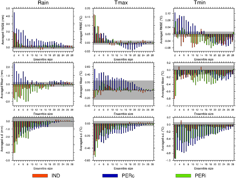
Figure 1. Difference between the full 30-member ensemble and the given sub-ensemble for the spatial average RMSE, mean and standard deviation (s.d.). The sub-ensembles are formed from the top ranking members determined using either an independence (IND), or performance (climatological, PERc, or impact, PERi) based measure. The gray region represents 1%, 1% and 5% of the full ensemble value respectively.
Download figure:
Standard image High-resolution image
It is not surprising that the performance measure based sub-ensembles to not reproduce the ensemble standard deviation as well as the independence based sub-ensemble, as it is generally expected to reduce the spread of the ensemble. Indeed, an 8-member IND sub-ensemble reproduces the ensemble standard deviation while 18 and 22 members are required for PERi and PERc respectively. The performance measures are however designed to minimize error, here given by the RMSE. In order to reproduce the full ensemble performance in terms of the RMSE, sub-ensembles of 7 members are required for both the IND and the PERi, while PERc requires up to 17 members. Thus even against the ensemble characteristic for which the performance measures should excel, the independence measure does just as well. Finally, to reproduce the ensemble mean 6 IND members are required while 9 (10) PERi (PERc) members are needed. This confirms that the independence measure chosen is acting as expected in terms of selecting an un-biased sub-sample.
These results demonstrate that using an independence measure is preferable to performance measures when creating small ensembles with characteristics that reflect those of larger ensembles. This is the first example of the use of a quantitative model independence measure to choose sub-ensembles and represents a significant step forward in the application of a model independence measure to climate model ensembles. While the robustness of this result requires further testing on other datasets and against other performance measures, it has implications for the analysis of climate model ensembles and the creation of downscaled climate projections.
Many studies based on subsets of the CMIP5 dataset are now being published in the literature. How representative the results of these studies are to the full dataset is difficult to determine. Using the independence ranking of the full CMIP5 ensemble one can place the ensemble subset for any particular study within the full ensemble. That is, if the subset contains a large enough group of the highest independence ranked models then it will have characteristics that reflect the full ensemble. On the other hand, if the subset contains mostly low ranked models then the results are unlikely to reflect those from the full ensemble.
The methodology presented here is perhaps most pertinent to dynamical downscaling studies, where significant computational costs restricts the number of downscaling experiments that can be made. Thus for dynamical downscaling studies, the independence measure can be used to guide the selection of global models in order to retain the key statistical characteristics of the full global model ensemble in the downscaled projections.
Acknowledgments
This work was made possible by funding from the Australian Research Council as part of the Future Fellowship FT110100576 and Linkage project LP120200777, and was supported by an award under the Merit Allocation Scheme on the NCI National Facility at the Australian National University. This work is a contribution to the NARCliM project.